Inclined Layer Method-Based Theoretical Calculation of Active Earth Pressure of a Finite-Width Soil for a Rotating-Base Retaining Wall

Abstract

In this study, we evaluated the active earth pressure on a retaining wall with a narrow cohesive fill under the rotation about the base mode. Under these conditions, Rankine’s and Coulomb’s earth pressure theories are not strictly effective. To improve the traditional earth pressure calculation methods (Rankine and Coulomb methods) and deduce the active earth pressure under the rotation about the base mode, here, we propose a new calculation method that incorporates the effects of wall displacement, soil arching and soil cohesion using inclined thin-layer elements. The calculation results are in good agreement with the model test data. Based on the parameter analysis, a critical aspect ratio of B/H = cotβ is determined along with a detailed elucidation of the various influencing factors (such as aspect ratio, cohesion and friction angle). The paper presents several solutions to improve the stability and lower the costs of retaining walls.

1. Introduction

Retaining walls are extensively used in bridges, slopes and tunnels to retain soil and protect the surrounding buildings because of their uncomplicated structures and low costs. Rankine’s method [1] and Coulomb’s theory [2] are widely used for designing retaining structures. However, some underlying problems have been encountered with the traditional earth pressure calculation methods; for instance, the classical earth pressure theory uses the same method to calculate the active earth pressure of the rotating retaining structures [3] and the translational (T) walls. However, experiments [4] show that the distribution of earth pressure in rotational mode is completely different from that in T mode. Therefore, the classical earth pressure theory is not completely suitable for earth pressure design and calculation of rotary retaining walls. To overcome this limitation, some scholars have estimated the retaining-wall earth pressure under displacement modes of rotation around the wall bottom (RB) and rotation around the wall top (RT) [5,6,7,8,9]. In addition, the retaining wall is inevitably built near natural rocks and supporting structures, which form a confined filling between the retaining wall and the existing support [10,11]. The traditional theory assumes that the backfill behind the wall is a soil with a semi-infinite width. However, this assumption is not applicable to a narrow backfill, and therefore, it is essential to develop a new method for calculating the active earth pressure of a soil with a finite width under the RB mode.

In recent years, researchers have tested retaining walls under different displacement modes (T, RB and RT) to study the load transfer law [12,13,14,15]. The experimental data revealed that the soil arching effect caused by wall–soil friction results in a non-linearly distributed earth pressure on the wall back [16]. Further, the distribution of earth pressure is largely affected by the wall displacement mode [17]. Although the earth pressure distribution law of a rotational retaining wall is significantly different from that of a translational wall, the current research on earth pressure is mostly focused on translational retaining walls [18,19,20,21]. Therefore, it is necessary to study the distribution law of soil pressure under the RB mode. In addition, soil cohesion, which is one of the two indicators of shear strength, largely affects the magnitude of the earth pressure. However, the mechanism influence of soil cohesion on earth pressure has rarely been studied to date.

To calculate the earth pressure, most researchers assume that the soil reaches a limit equilibrium state, and the shear strength of the backfill is fully exerted without taking displacement into account [22]. However, in actual engineering, the retaining wall is in a nonlimit state, and its displacement affects the distribution of soil pressure [23]. Experiments show that the effective value of shear strength changes with depth in the nonlimit state [24]. This change in the effective shear strength is required for calculating the earth pressure to establish a functional relationship between the shear strength and displacement. In a previous study, a linear relationship was reported between the friction angle and displacement [25].

Under the framework of the limit equilibrium theory, two theoretical calculation methods are used to explore the stress state of the fill, viz., the sliding soil wedge method and the horizontal differential element method. The sliding soil wedge method has natural advantages based on the Coulomb theory, but it cannot reflect the soil pressure distribution [26]. Accordingly, the horizontal differential element method is more practical, because it considers the soil arching effect. However, this method does not consider the shear stress that makes the element stress unbalanced in the horizontal direction [27], and produces an uneven stress distribution at the upper and lower interfaces of the element [28,29]. Thus, to overcome the limitations of these methods, significant improvements are required.

In this study, we developed a calculation method that considers the wall displacement, soil arching effect and soil cohesion to deduce the active earth pressure under the RB mode. A detailed analysis was conducted to validate the reliability of this method, along with an in-depth evaluation of soil properties to indicate various measures to effectively reduce soil pressure and improve the stability of retaining walls. The primary objectives of this study were: (a) to present a new method for calculating the earth pressure of a narrow fill, and (b) to provide viable solutions for improving retaining-wall designs.

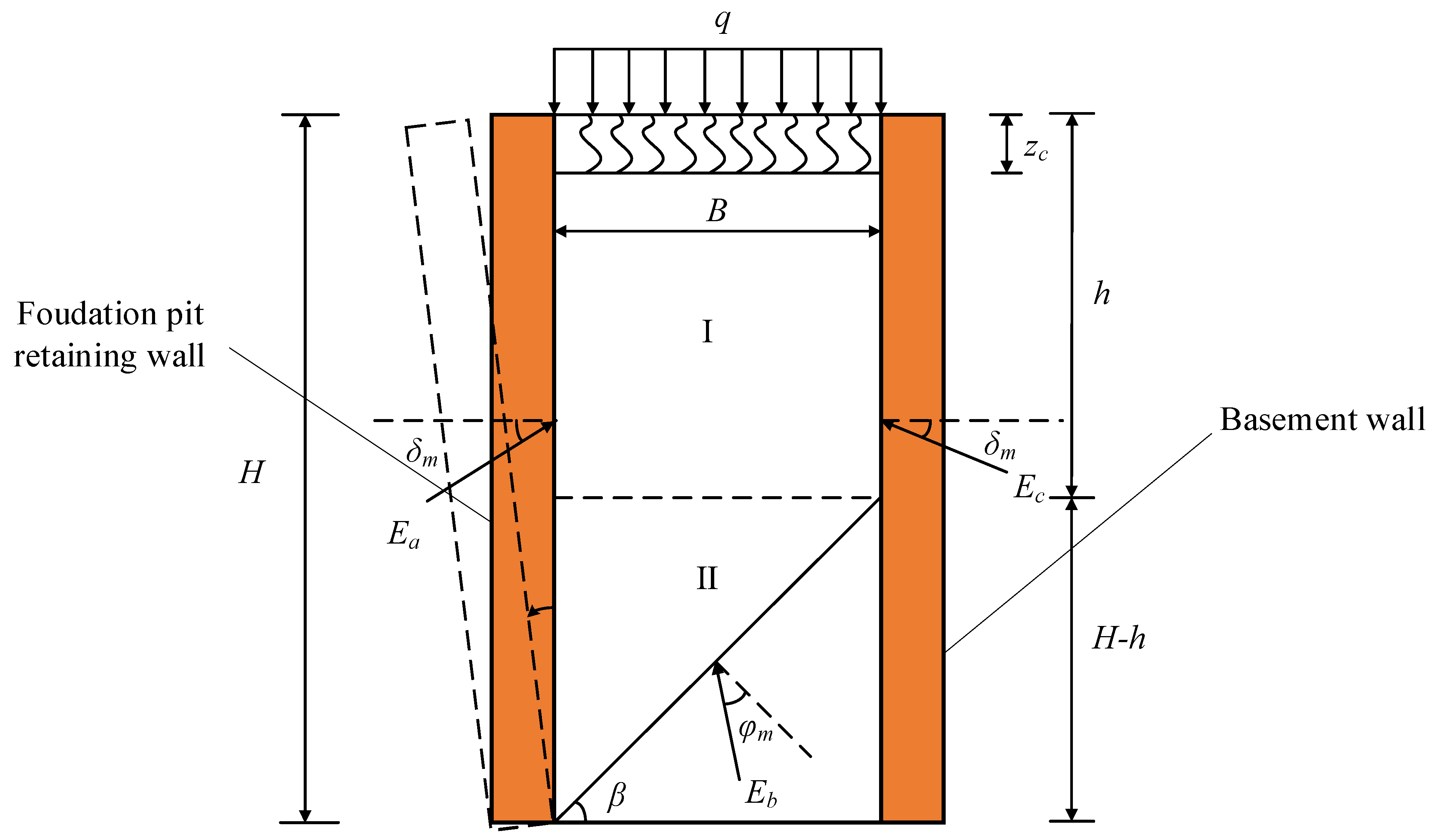
2. Basic Hypothesis

Figure 1 shows a schematic of the finite-width soil behind a retaining wall, used for the stress analysis in this study. As shown in Figure 1, the finite-width clay behind the retaining wall forms a slip surface under the RB displacement mode. The sliding surface intersects the basement wall at a point, and the wedge is divided into zone I (rectangular space) and zone II (triangular space) by the horizontal line passing through this point. The heights of zone I and zone II are h and H-h, respectively, and $h=H-B\tan \beta$, where $\beta$ is the rupture angle. Previous experiments [14,30] showed that the slip surface of a retaining wall basically follows Rankine’s theory, we have

$$\beta ={45}^{\circ }+\phi /2$$

(1)

Figure 1. Schematic of the finite-width soil behind a retaining wall.

For the theoretical calculations in this study, the following assumptions were made:

(1)

The clay behind the wall is of the same material, the soil’s cohesion is c, and the friction angle of the soil is φ. In addition, the developed value of φ is φ_m.

(2)

The basement wall does not move, and the foundation-pit retaining wall rotates outward around the wall base.

(3)

The Mohr–Coulomb criterion governs the shear strength of the soil with a finite width.

(4)

The roughness of the wall back is taken into account, and the wall–soil friction angles of both the foundation-pit retaining wall and the basement exterior wall are δ. Therefore, the effective value of δ is δ_m.

(5)

The wall–soil cohesion of the retaining-wall foundation pit and that of the basement wall is c_w and c_d, respectively.

(6)

The soil on the ground surface has a uniform load q (unit: kN/m).

(7)

A straight slip surface is assumed across the wall heel.

3. Determination of Friction Angle and Soil’s Cohesion in the Nonlimit State

3.1. Qualitative Analysis of Nonlimit State

In applying the classical earth pressure theory, engineers and technicians assume that the soil displacement behind the wall reaches its ultimate state; this is then reduced by applying a safety factor. However, the wall often fails to reach the limiting condition [24,31]. Bang [32] first proposed the nonlimit state hypothesis, which holds that an intermediate state between the static and limiting states of the retaining wall exists, which is referred to as the nonlimit state. Nonlimit earth pressure is affected by factors such as retaining wall displacement mode and fill displacement, and the calculation is very complex [33,34]. At present, it is in the exploratory stage. Relevant research is of great significance to ensure the stability of retaining walls and to optimize structural design [35].

The model experiments of Sherif [36] and Xu [37], as well as the FEM results of Matsuzawa [38] and Naikai [39], demonstrated that as the wall rotation under RB increased, the earth pressure at different depths declined sharply and then gradually stabilized. The backfill soil entered the limit equilibrium state from top to bottom.

The resultant force of ground pressure diminishes as the rotation angle increases in RB mode. The displacement of the retaining wall increases with the increase in the wall rotation. Sherif et al. [36] proposed $S_c$ as the critical value of the displacement of the soil behind the retaining wall, reaching the active limit state. Fang et al. [24] suggested $S_c=3~5\times {10}^{-4}$ H for sandy soil, with H as the wall height, and the value of $S_c$ was only dependent on the wall height. It is assumed that $S_{\mathrm{d}}$ refers to the horizontal displacement of the soil behind the wall top when the wall rotates. When $S_{\mathrm{d}}/S_c<1$, the soil within the wall height is in the nonlimit state; when $S_{\mathrm{d}}/S_c=1$, the soil at the top of the wall just reaches the active limit state; when $S_{\mathrm{d}}/S_c>1$, the active limit state begins to extend downward from the top of the wall with the increase in the angle of the rigid wall, and the earth pressure continuously decreases. Because the rotation angle is large enough, the shear strength of the soil can be thoroughly developed. Moreover, the rotation angle continues to increase, soil pressure behind the wall remains constant, and active limit states stop propagating downward.

3.2. Calculation of Shear Strength Parameters in Nonlimit State

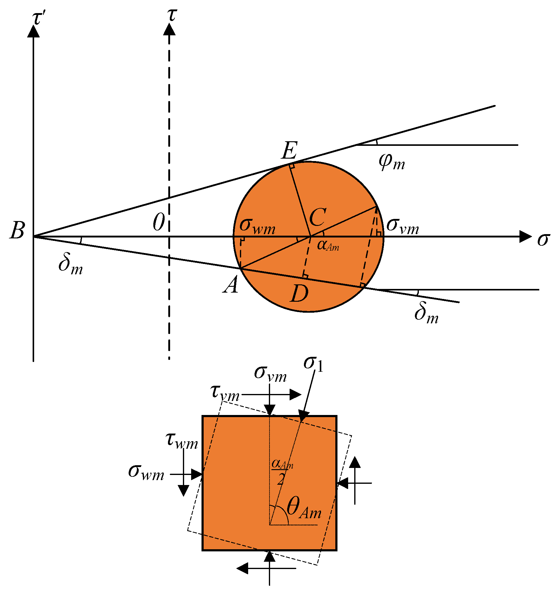
3.2.1. Calculation of Friction Angle Parameters

Xu et al. [40] derived the theoretical formula of soil friction angle ${\phi }_{\mathrm{m}}$ on a displaced wall in the nonlimit state using the Mohr stress circle as:

$$\sin {\phi }_{\mathrm{m}}=\frac{(1-R_{\mathrm{f}}+\eta R_{\mathrm{f}})(1-K_0)(1+\sin \phi )+\eta \sin \phi (1+K_0)-\eta (1-K_0)}{(1-R_{\mathrm{f}}+\eta R_{\mathrm{f}})(1+K_0)(1+\sin \phi )-\eta \sin \phi (1+K_0)+\eta (1-K_0)}$$

(2)

where $R_{\mathrm{f}}$ is the failure ratio with a value in the range of 0.75–1.00. For a normal consolidated soil, the initial value of soil friction angle can be calculated by the following formula:${\phi }_0=\arcsin \left[{(1 - \mathrm{K}}_0{)/(1+\mathrm{K}}_0)\right]$. For normally consolidated soil, the static earth-pressure coefficient (K₀) is given by: $K_0=0.95-\sin \phi$ [41]. Suppose $S_{\mathrm{z}}$ is the horizontal displacement of the wall at a certain depth under the active state, and $S_{\mathrm{c}}$ is the horizontal displacement of the retaining wall at any height under the active limit state. Then, the displacement ratio of the retaining wall, η, can be calculated by $\eta =S_{\mathrm{z}}/S_{\mathrm{c}}$. The critical horizontal displacement of the cohesive soil, $S_{\mathrm{c}}$, ranges from 0.4% H to 1.0% H [42].

Gong et al. [31] proposed a method for calculating the effective value of the wall–soil friction angle as follows:

$$\tan {\delta }_{\mathrm{m}}=\tan {\delta }_0+\frac{4}{\pi }(\arctan \eta )(\tan \delta -\tan {\delta }_0)$$

(3)

Chang [25] proposed that the initial wall–soil friction angle ${\delta }_0$ could be replaced by $\phi /2$. Moreover, the wall–soil friction angle $\delta$ is the experimentally measured value, which can be replaced by $2\phi /3$ in the absence of experimental data [43].

3.2.2. Calculation of Cohesion Parameters

In previous studies, a functional relationship between the friction angle and displacement was established. However, only a few methods for calculating the cohesion parameters have been reported to date. In this study, we established a relationship between cohesion and the friction angle; this makes cohesion indirectly relate to the wall displacement. Here, the fully developed value of adhesion force between the foundation-pit retaining wall and the soil is $c_{\mathrm{w}}$, and that between the basement wall and the soil is $c_{\mathrm{d}}$, and $c_{\mathrm{w}}$ and $c_{\mathrm{d}}$ can be calculated from $2c/3$. In addition, the developed values of the wall–soil adhesion force can be obtained as follows [44].

$$c_{\mathrm{wm}}=c_{\mathrm{w}}\tan {\delta }_{\mathrm{m}}/\tan \delta$$

(4)

$$c_{\mathrm{dm}}=c_{\mathrm{d}}\tan {\phi }_{\mathrm{m}}/\tan \phi$$

(5)

In this formula, $c_{\mathrm{wm}}$ is the developed value of the cohesive force between the retaining wall and the soil, and $c_{\mathrm{dm}}$ is the developed value of the adhesive force between the basement wall and the soil. In addition, ${\delta }_{\mathrm{m}}$ is the effective value of the wall–soil friction angle, and ${\phi }_{\mathrm{m}}$ is the developed value of the soil friction angle.

Based on the derived calculation formula of cohesion under the nonlimit state, we can obtain the expression of shear stress for zone I as:

$${\tau }_{\mathrm{wm}}=c_{\mathrm{w}}\frac{\tan {\delta }_m}{\tan {\delta }_{}}+{\sigma }_{\mathrm{wm}}\tan {\delta }_{\mathrm{m}}$$

(6)

$${\tau }_{\mathrm{sm}}=c_{\mathrm{d}}\frac{\tan {\delta }_m}{\tan \delta }+{\sigma }_{\mathrm{sm}}\tan {\delta }_{\mathrm{m}}$$

(7)

where ${\sigma }_{\mathrm{wm}}$ and ${\tau }_{\mathrm{wm}}$ are the normal stress and shear stress of the soil at the contact between the foundation-pit retaining wall and the soil, respectively; ${\sigma }_{\mathrm{sm}}$ and ${\tau }_{\mathrm{sm}}$ are the normal stress and shear stress of the soil at the contact between the basement wall and the backfill, respectively.

4. Derivation of Active Earth Pressure of a Finite-Width Soil

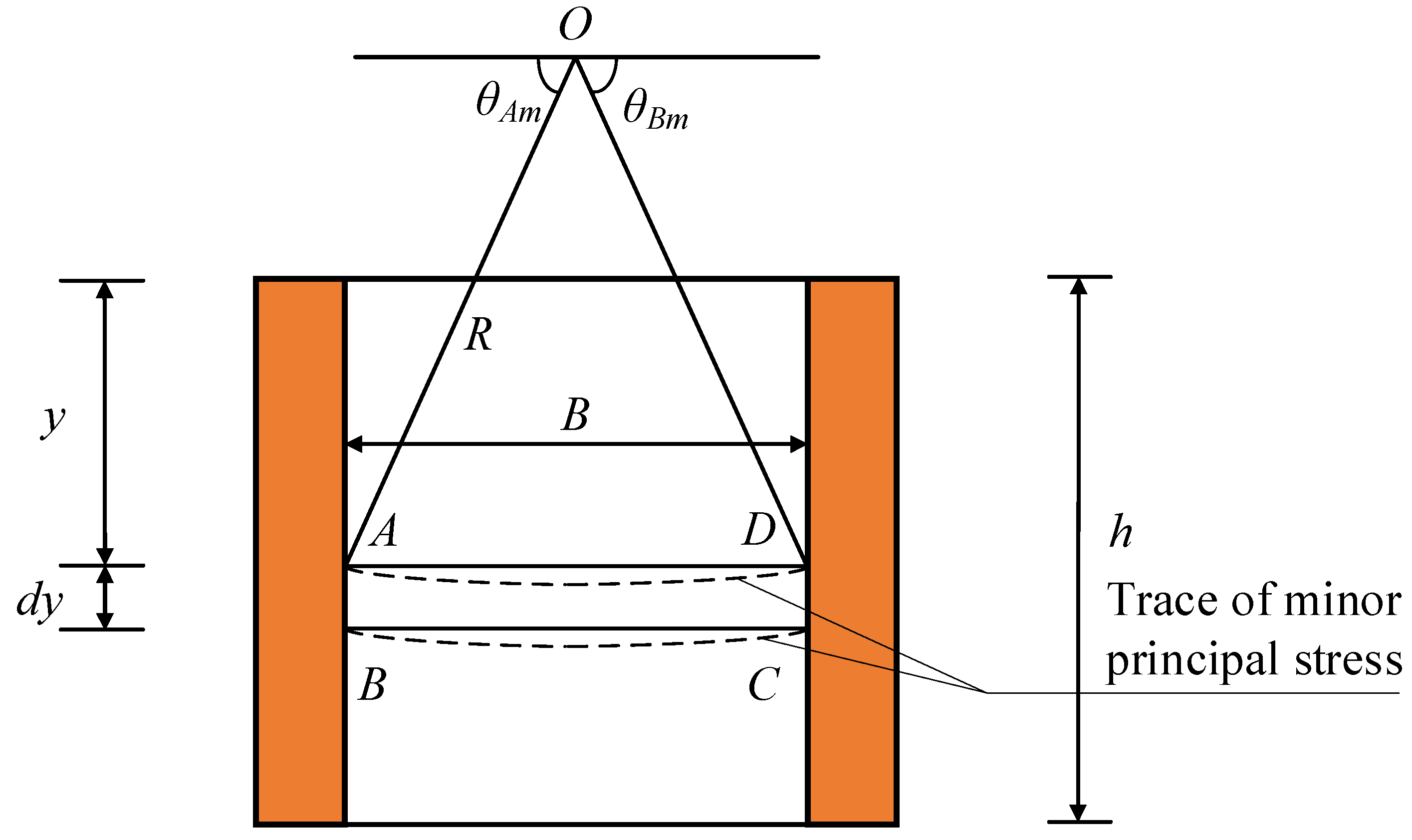
4.1. Principal Stress Trajectory

Due to the existence of wall–soil friction, the principal stress is no longer just transmitted horizontally or vertically; instead, it is deflected, and the corresponding direction can be expressed using the principal stress trace [29]. There are various forms of principal stress traces, such as parabola, catenary and arc. In addition, Smita [45] found that the shape of the principal stress trace has a negligible effect on the calculated results of earth pressure, and thus, can be ignored. Therefore, to simplify the calculations, the arc principal stress trace was adopted in this study. As shown in Figure 2, an inclined line can be obtained by connecting the trace of the small principal stress in zone I with the intersection point of the walls on both sides, which can replace the trace of the small principal stress. Because the friction coefficient between the foundation-pit retaining wall and the soil and that between the basement wall and the soil is the same, i.e., $\delta$, the principal stress trace in zone I can be expressed by horizontal lines.

Figure 2. Trajectory of the minor principal stress in zone I.

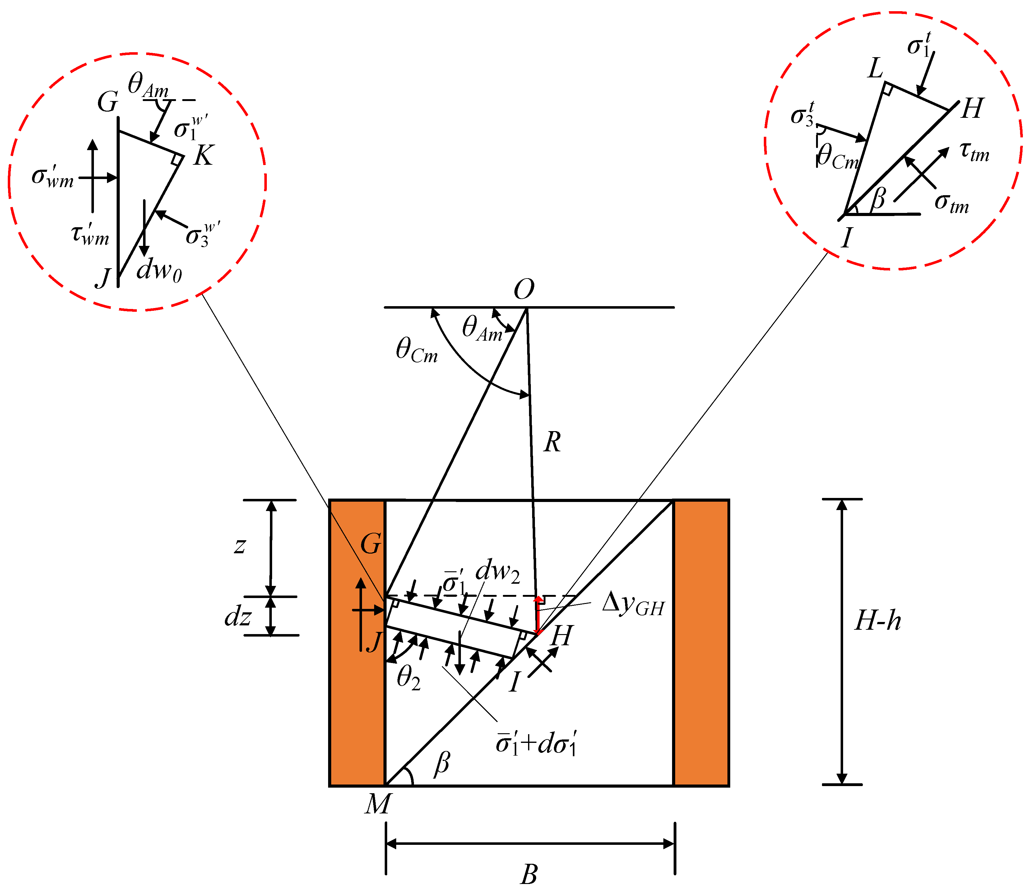
4.2. Derivation of Active Earth Pressure in Rectangular Area

Zone I is a rectangular region that does not contain a slip surface, as shown in Figure 3. At a depth y from the ground level, a thin-layer element ABCD with a thickness of dy is considered for the static analysis.

Figure 3. Stress analysis model of zone I.

It is assumed that the normal stress of the soil at the contact between the retaining wall and the soil is ${\sigma }_{\mathrm{wm}}$, and the shear stress is ${\tau }_{\mathrm{wm}}$. Further, the normal stress of the soil at the junction of the basement wall and the soil is ${\sigma }_{\mathrm{sm}}$, and the shear stress is ${\tau }_{\mathrm{sm}}$.

The major and minor principal stresses of the soil at the contact between the soil and the retaining wall are ${\sigma }_1^{\mathrm{w}}$ and ${\sigma }_3^{\mathrm{w}}$, respectively. In addition, the major and minor principal stresses of the soil at the interface between the soil and the basement wall are ${\sigma }_1^{\mathrm{s}}$ and ${\sigma }_3^{\mathrm{s}}$, respectively.

As shown in Figure 3, the triangular elements ΔABE and ΔCDF are considered at the contact between the retaining wall and the soil and the junction between the basement wall and the soil, respectively. The following conclusions can be obtained by applying the static equilibrium theory:

$${\sigma }_{\mathrm{wm}}={\sigma }_3^{\mathrm{w}}{\sin }^2{\theta }_{\mathrm{Am}}+{\sigma }_1^{\mathrm{w}}{\cos }^2{\theta }_{\mathrm{Am}}$$

(8)

$${\tau }_{\mathrm{wm}}=({\sigma }_1^{\mathrm{w}}-{\sigma }_3^{\mathrm{w}})\sin {\theta }_{\mathrm{Am}}\cos {\theta }_{\mathrm{Am}}$$

(9)

$${\sigma }_{\mathrm{sm}}={\sigma }_1^{\mathrm{s}}{\sin }^2(\pi -{\theta }_{\mathrm{Bm}})+{\sigma }_3^{\mathrm{w}}{\cos }^2(\pi -{\theta }_{\mathrm{Bm}})$$

(10)

$${\tau }_{\mathrm{sm}}=({\sigma }_1^{\mathrm{s}}-{\sigma }_3^{\mathrm{s}})\sin (\pi -{\theta }_{\mathrm{Bm}})\cos (\pi -{\theta }_{\mathrm{Bm}})$$

(11)

where ${\theta }_{\mathrm{Am}}$ is the cut angle between the maximum principal stress and the horizontal direction at the interface between the retaining wall and the soil in zone I. In addition, ${\theta }_{\mathrm{Bm}}$ represents the angle between the maximum principal stress and the horizontal direction at the interface between the basement wall and the soil in zone I.

According to the Mohr–Coulomb criterion, the following functional relationship can be established between the major and minor principal stresses of cohesive soils [46]:

$$N=\frac{{\sigma }_1^{\mathrm{s}}+c\cot \phi }{{\sigma }_3^{\mathrm{s}}+c\cot \phi }=\frac{{\sigma }_1^{\mathrm{w}}+c\cot \phi }{{\sigma }_3^{\mathrm{w}}+c\cot \phi }={\tan }^2({45}^{\circ }+\frac{\phi }{2})$$

(12)

where the magnitude of N is only related to the soil friction angle, and has no relation with the wall height H, soil width B and cohesion c.

To obtain the solutions of the principal stress deflection angles ${\theta }_{\mathrm{Am}}$ and ${\theta }_{\mathrm{Bm}}$, as shown in Figure 4, the Mohr stress circle is employed.

Figure 4. Mohr’s stress circle model of the backfill.

The following equation is derived from the geometric relationship shown in Figure 4:

$${\theta }_{\mathrm{Am}}+\frac{{\alpha }_{\mathrm{Am}}}{2}=\frac{\pi }{2}$$

(13)

where ${\alpha }_{\mathrm{Am}}/2$ is the cut angle between the major principal stress and the vertical direction.

Figure 4 shows the geometrical relationship of the Mohr stress circle.

$$\angle CBE={\phi }_{\mathrm{m}}$$

(14)

$$\angle CBA={\delta }_{\mathrm{m}}$$

(15)

$$\angle BCA={\alpha }_{\mathrm{Am}}$$

(16)

$$\sin ({\delta }_{\mathrm{m}}+{\alpha }_{\mathrm{Am}})=\frac{\overline{CD}}{\overline{AC}}=\frac{\overline{CD}}{R}$$

(17)

$$\sin {\delta }_{\mathrm{m}}=\frac{\overline{CD}}{\overline{BC}}$$

(18)

$$\sin {\phi }_{\mathrm{m}}=\frac{\overline{CE}}{\overline{BC}}=\frac{R}{\overline{BC}}$$

(19)

where ${\phi }_{\mathrm{m}}$ is the effective value of the soil friction angle; ${\delta }_{\mathrm{m}}$ is the effective value of the wall–soil friction angle; and R is the radius of the Mohr stress circle.

Combining Equations (17)–(19), we have

$$\sin ({\delta }_{\mathrm{m}}+{\alpha }_{\mathrm{Am}})=\frac{\sin {\delta }_{\mathrm{m}}}{\sin {\phi }_{\mathrm{m}}}$$

(20)

The simultaneous Equations (13) and (20) can be used to deduce the expression of the principal stress deflection angle.

$$\{\begin{array}{l}{\theta }_{\mathrm{Am}}={\theta }_{\mathrm{Bm}}=\frac{\pi }{2}-u\\ u=\frac{1}{2}\left[\arcsin (\sin {\delta }_{\mathrm{m}}/\sin {\phi }_{\mathrm{m}})-{\delta }_{\mathrm{m}}\right]\end{array}$$

(21)

Because of the same friction coefficient on both sides of the retaining wall, the principal stress deflection angle satisfies the following condition: ${\theta }_{\mathrm{Am}}$ = ${\theta }_{\mathrm{Bm}}$.

As shown in Figure 2, the geometric parameters of the thin-layer differential element can be determined by the following method. The left and right interfaces of the unit are line segments $l_{AB}$ and $l_{CD}$, and the lengths are all dy. The intersections of the principal stress trace and the wall on both sides are represented by points A and D, respectively, and the line $l_{AD}$ is obtained by connecting two points at a depth y from the filling surface. Further, $l_{AD}$ represents the length of the upper interface of the thin layer unit. At a depth of y+dy from the ground surface, the lower interface of the unit $l_{BC}$ can be obtained in the same way. Because the friction coefficients of the wall back of the foundation-pit retaining wall and the basement wall are equal, the principal stress traces are symmetrical. Therefore, points A and D are on the same horizontal line, and points B and C are also on the same horizontal line. Based on this, the following relationship can be obtained:

$$l_{AB}=l_{CD}=dy$$

(22)

$$l_{AD}=l_{BC}=B$$

(23)

As depicted in Figure 3, the major principal stress is uniformly distributed at the upper and lower interfaces of the thin-layer element. Thus,

$${\sigma }_1^{\mathrm{w}}={\sigma }_1^{\mathrm{s}}$$

(24)

The average principal stress ${\overline{\sigma }}_1$ acting on $l_{AD}$ is

$${\overline{\sigma }}_1=\frac{{\sigma }_1^{\mathrm{w}}+{\sigma }_1^{\mathrm{s}}}{2}={\sigma }_1^{\mathrm{w}}={\sigma }_1^{\mathrm{s}}$$

(25)

The force $F_{AD}$ on the upper interface of the thin-layer element can be expressed as:

$$F_{AD}=l_{AD}{\sigma }_1^{\mathrm{w}}$$

(26)

Similarly, the lower interface force ($F_{BC}$) of the thin-layer element is

$$F_{BC}=l_{BC}({\overline{\sigma }}_1+\mathrm{d}{\sigma }_1)$$

(27)

where ${\overline{\sigma }}_1+\mathrm{d}{\sigma }_1$ represents the stress acting on $l_{BC}$.

The tangential force $F_{AB}$ on the left interface of the thin-layer element of the soil can be expressed as:

$$F_{AB}=l_{AB}{\tau }_{\mathrm{wm}}$$

(28)

Similarly, the tangential force $F_{CD}$ on the right interface of the element is

$$F_{CD}=l_{CD}{\tau }_{\mathrm{sm}}$$

(29)

Further, gravity ${\mathrm{dw}}_1$ analysis of the thin-layer unit was performed, and the corresponding equation is as follows:

$${\mathrm{dw}}_1=\gamma \frac{(l_{AD}+l_{BC})t_1}{2}=\gamma Bdy$$

(30)

where t₁ is the thickness of the thin-layer unit; $\gamma$ is the unit weight of the soil; dy is the thickness of the element ABCD; and B is the soil width.

As the thin-layer element satisfies the static equilibrium conditions in the vertical and horizontal directions, the following equations can be obtained:

$${\sigma }_{\mathrm{wm}}{l}_{AB}-{\sigma }_{\mathrm{sm}}{l}_{CD}=0$$

(31)

$$F_{BC}+F_{AB}+F_{CD}-F_{AD}-{\mathrm{dw}}_1=0$$

(32)

Combining Equations (6), (7), (25), (31) and (32), we have

$$B\mathrm{d}{\sigma }_1+2c_{\mathrm{w}}\frac{\tan {\delta }_{\mathrm{m}}}{\tan \delta }dy+2\tan {\delta }_{\mathrm{m}}{\sigma }_{\mathrm{wm}}dy-\gamma Bdy=0$$

(33)

Equation (33) contains two unknowns ${\sigma }_1$ and ${\sigma }_{\mathrm{wm}}$; thus, in this study, we considered the simultaneous Equations (8) and (12) to eliminate ${\sigma }_{\mathrm{wm}}$, and the derivation process is as follows:

$$\begin{array}{l}{\sigma }_{\mathrm{wm}}=({\sigma }_3^{\mathrm{w}}+c\cot \phi ){\sin }^2{\theta }_{\mathrm{Am}}-c\cot \phi {\sin }^2{\theta }_{\mathrm{Am}}\\ +({\sigma }_1^{\mathrm{w}}+c\cot \phi ){\cos }^2{\theta }_{\mathrm{Am}}-c\cot \phi {\cos }^2{\theta }_{\mathrm{Am}}\end{array}$$

(34)

A functional relationship between ${\sigma }_{\mathrm{wm}}$ to ${\sigma }_1$ can be obtained by simplifying Equation (34).

$${\sigma }_{\mathrm{wm}}=t_3({\sigma }_1^{}+c\cot \phi )-c\cot \phi$$

(35)

$$t_3=\frac{{\sin }^2{\theta }_{\mathrm{Am}}}{N}+{\cos }^2{\theta }_{\mathrm{Am}}$$

(36)

where t₃ is the accommodation coefficient of ${\sigma }_1^{}$.

The differential equation of ${\sigma }_1$ can be obtained by combining Equations (33)–(36) as:

$$\frac{d{\sigma }_1^{}}{dy}+A_1{\sigma }_1^{}=A_2$$

(37)

$$A_1=\frac{2t_3\tan {\delta }_{\mathrm{m}}}{B}$$

(38)

$$A_2=\gamma -2\frac{c_{\mathrm{w}}\frac{\tan {\delta }_{\mathrm{m}}}{\tan \delta }+\tan {\delta }_{\mathrm{m}}c\cot \phi (t_3-1)}{B}$$

(39)

where A₁ and A₂ are the relevant parameters of the differential equation about ${\sigma }_1$.

By solving the above differential equation, we obtain

$${\sigma }_1=C_1{e}^{-A_1\mathrm{y}}+\frac{A_2}{A_1}$$

(40)

where C₁ is an undetermined coefficient.

By substituting Equation (40) into Equation (35), the active earth pressure strength of zone I can be derived as:

$${\sigma }_{\mathrm{wm}}=C_1{t}_3{e}^{-A_1\mathrm{y}}+A_3$$

(41)

$$A_3=t_3\frac{A_2}{A_1}+(t_3-1)c\cot \phi$$

(42)

where A₃ is the constant term of the general solution of the differential equation; where C₁ is an undetermined coefficient, which can be calculated according to the boundary conditions applicable at the top of the foundation-pit retaining wall.

As shown in Figure 5, the triangular element ΔVPT can be taken for the analysis of the wall–soil interface at the top of the foundation-pit retaining wall. Here, VT coincides with the back of the wall, VP coincides with the top of the retaining wall, and PT coincides with the direction of the major principal stress at point V. The normal stress and shear stress on the left interface of ΔVPT are ${\sigma }_{\mathrm{wv}}$ and ${\tau }_{\mathrm{wv}}$, respectively. The stress on the right interface is ${\sigma }_3^v$, and that on the upper interface is q. Because the line length of the triangle is very short, it can be considered that the principal stress is approximately uniformly distributed at the interface of the element.

$${\sigma }_{\mathrm{wv}}{l}_{VT}-{\sigma }_3^v{l}_{PT}\sin {\theta }_{\mathrm{Am}}=0$$

(43)

$${\tau }_{\mathrm{wv}}{l}_{VT}+{\sigma }_3^v{l}_{PT}\cos {\theta }_{\mathrm{Am}}-q{l}_{PV}=0$$

(44)

where ${\theta }_{\mathrm{Am}}$ is the cut angle between the major principal stress and the horizontal direction. In addition, $l_{VT}$, $l_{PT}$ and $l_{PV}$ are the lengths of the lines VT, PT and PV, respectively.

$$\{\begin{array}{l}{l}_{VT}=dy\\ l_{PT}=dy/\sin {\theta }_{\mathrm{Am}}\\ l_{PV}=dy\cot {\theta }_{\mathrm{Am}}\end{array}$$

(45)

Figure 5. Force analysis of the unit—ΔVPT.

Combining Equations (43)–(45), we obtain

$${\sigma }_{\mathrm{wv}}={\lambda }_{ 1}q-{\lambda }_{ 2}{c}_{\mathrm{w}}$$

(46)

$${\lambda }_1=\frac{\cot {\theta }_{\mathrm{Am}}}{\tan {\delta }_{\mathrm{m}}+\cot {\theta }_{\mathrm{Am}}}$$

(47)

$${\lambda }_2=\frac{\tan {\delta }_{\mathrm{m}}}{(\tan {\delta }_{\mathrm{m}}+\cot {\theta }_{\mathrm{Am}})\tan \delta }$$

(48)

where ${\sigma }_{\mathrm{wv}}$ indicates the lateral earth pressure of the retaining wall at the filling depth of y = 0. In addition, $c_{\mathrm{w}}$ is the stick force between the foundation-pit retaining wall and the soil. Lastly, λ₁ and λ₂ are the adjustment coefficients of q and c_w, respectively.

According to the boundary conditions, when y = 0, we obtain ${\sigma }_{\mathrm{wm}}={\sigma }_{\mathrm{wv}}$. The expression of the undetermined coefficient C₁ can be calculated using this boundary condition.

$$C_1=\frac{{\lambda }_{ 1}q-{\lambda }_{ 2}{c}_{\mathrm{w}}-A_3}{t_3}$$

(49)

When the retaining wall moves in the RB mode, tensile cracks form in the soil near the top of the wall. The depth of the fractured space, $z_c$, can be obtained under the condition that the lateral earth pressure of zone I is zero [47].

$$z_c=-\frac{1}{A_1}\ln (-\frac{A_3}{C_1{t}_3})$$

(50)

When $h>z_c$, the depth of the tension crack is completely inside zone I, and the active earth pressure resultant force in zone I is $E_{a1}$.

$$E_{a1}={\int }_{z_c}^h{\sigma }_{\mathrm{wm}}dy$$

(51)

Further, the active earth pressure tilting moment $M_1$ of the retaining wall can be denoted as:

$$M_1={\int }_{z_c}^h{\sigma }_{\mathrm{wm}}(H-y)dy$$

(52)

When $h\le z_c$, the tension crack extends from the fill surface to zone II, and the resultant force of the active earth pressure $E_{a1}$ as well as the overturning torque $M_1$ are both zero.

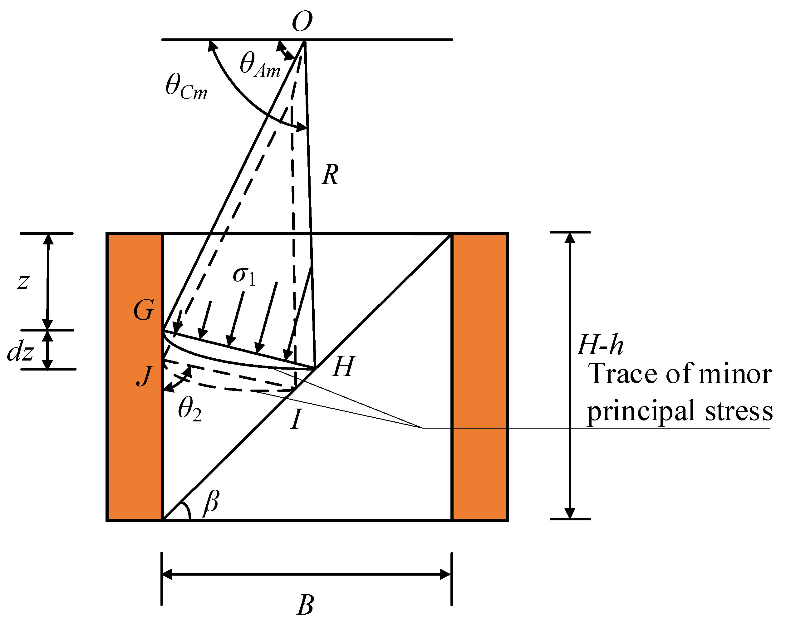
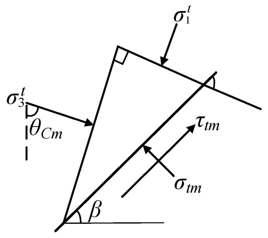
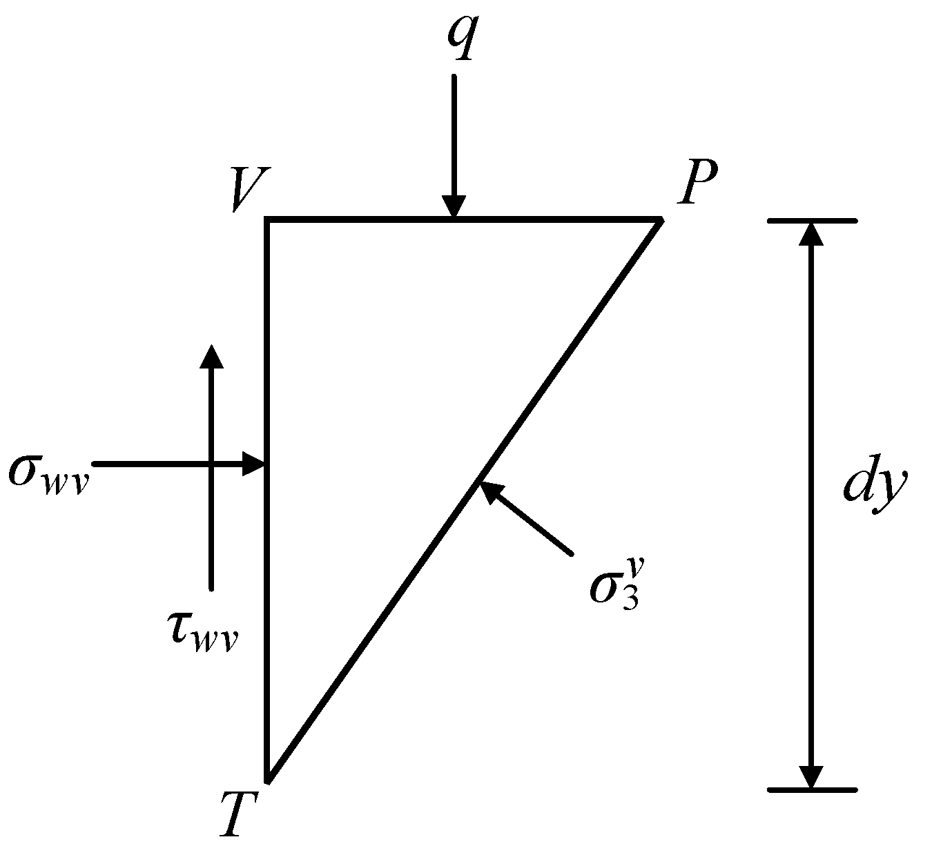
4.3. Derivation of Active Earth Pressure in Triangular Area

As depicted in Figure 6, the zone II earth pressure analysis model includes a slip surface. Thus, it can be considered as a triangular area for the analysis and calculation. Because the frictional coefficients of the left and right sides of the triangular soil wedge are different, the principal stress trace can be simplified as an inclined straight line, and an inclined thin-layer element GHIJ is obtained. It is generally believed that the soil arching effect changes only the direction of the principal stress transmission without changing its value. The change in the magnitude of the large principal stress ${\sigma }_1^{\prime }$ on the principal stress trajectory is determined by its burial depth [28].

Figure 6. Trajectory of minor principal stress of zone II.

As shown in Figure 7, we assume that the normal stress on the left interface of the thin-layer element is ${\sigma }_{\mathrm{wm}}^{\prime }$, and the shear stress is ${\tau }_{\mathrm{wm}}^{\prime }$. Further, the normal stress on the right interface of the thin-layer element is ${\sigma }_{\mathrm{t}\mathrm{m}}^{}$, and the shear stress is ${\tau }_{\mathrm{t}\mathrm{m}}$.

Figure 7. Stress analysis model of zone II.

The major and minor principal stresses of the soil at the contact between the soil and the retaining wall are ${\sigma }_1^{{\mathrm{w}}^{\prime }}$ and ${\sigma }_3^{{\mathrm{w}}^{\prime }}$, respectively. In addition, the major and minor principal stresses of the soil at the interface between the soil and the slip surface are ${\sigma }_1^t$ and ${\sigma }_3^t$, respectively.

Since triangular elements $\Delta GKJ$ and $\Delta HIL$ satisfy the static equilibrium conditions, we can obtain

$${\mathrm{w}}_{\mathrm{wm}}^{\prime }={\sigma }_3^{{\mathrm{w}}^{\prime }}{\sin }^2{\theta }_{\mathrm{Am}}+{\sigma }_1^{{\mathrm{w}}^{\prime }}{\cos }^2{\theta }_{\mathrm{Am}}$$

(53)

$${\tau }_{\mathrm{wm}}^{\prime }=({\sigma }_1^{{\mathrm{w}}^{\prime }}-{\sigma }_3^{{\mathrm{w}}^{\prime }})\sin {\theta }_{\mathrm{Am}}\cos {\theta }_{\mathrm{Am}}$$

(54)

$${\sigma }_{\mathrm{t}\mathrm{m}}={\sigma }_1^{\mathrm{t}}{\sin }^2({\theta }_{\mathrm{Cm}}-\beta )+{\sigma }_3^{\mathrm{t}}{\cos }^2({\theta }_{\mathrm{Cm}}-\beta )$$

(55)

$${\tau }_{\mathrm{t}\mathrm{m}}=({\sigma }_1^{\mathrm{t}}-{\sigma }_3^{\mathrm{t}})\sin ({\theta }_{\mathrm{Cm}}-\beta )\cos ({\theta }_{\mathrm{Cm}}-\beta )$$

(56)

where ${\theta }_{\mathrm{Am}}$ is the cut angle between the maximum principal stress and the horizontal direction at the interface between the retaining wall and the soil in zone II; ${\theta }_{\mathrm{Cm}}$ represents the angle between the maximum principal stress and the horizontal direction at the interface between the slip surface and the soil in zone II; and $\beta$ is the slip angle.

According to the Mohr–Coulomb criterion, the following functional relationship can be established between the major and minor principal stresses of the cohesive soils [46,48]:

$$N=\frac{{\sigma }_1^{{\mathrm{w}}^{\prime }}+\mathrm{c}\cot \phi }{{\sigma }_3^{{\mathrm{w}}^{\prime }}+\mathrm{c}\cot \phi }=\frac{{\sigma }_1^{\mathrm{t}}+\mathrm{c}\cot \phi }{{\sigma }_3^{\mathrm{t}}+\mathrm{c}\cot \phi }={\tan }^2({45}^{\circ }+\frac{\phi }{2})$$

(57)

where N is only related to the soil friction angle.

It can be seen from Figure 8 that the principal stress deflection angles ${\theta }_{\mathrm{Am}}$ and ${\theta }_{\mathrm{Cm}}$ can be represented as

$$\{\begin{array}{l}{\theta }_{\mathrm{Am}}=\frac{\pi }{2}-\frac{1}{2}\left[\arcsin (\sin {\delta }_{\mathrm{m}}/\sin {\phi }_{\mathrm{m}})-{\delta }_{\mathrm{m}}\right]\\ {\theta }_{\mathrm{Cm}}=\frac{\pi }{4}+\beta -\frac{\phi }{2}\end{array}$$

(58)

Figure 8. Geometric model of the principal stress deflection angle.

As shown in Figure 7, the inclined thin-layer element with a thickness dz is considered at a depth z from the top surface of zone II, and each side length of the element is calculated as follows:

$$l_{GJ}=dz$$

(59)

$$l_{KJ}=l_{IL}=dz\sin {\theta }_2$$

(60)

$$l_{HI}=\frac{dz\sin {\theta }_2}{\cos (\theta -\beta )}$$

(61)

where ${\theta }_2$ is the angle between the inclined thin-layer element and the vertical direction, and the length of the upper interface $l_{GH}$ of the inclined thin-layer can be calculated according to the geometrical relationship of ΔGHM shown in Figure 7.

$$l_{GH}=\frac{(H-h-z)\cos \beta }{\cos ({\theta }_2-\beta )}$$

(62)

Similarly, the length of the lower interface of the thin layer ($l_{IJ}$) can be obtained using the sine theorem.

$$l_{IJ}=\frac{(H-h-z-dz)\cos \beta }{\cos ({\theta }_2-\beta )}$$

(63)

Assuming that the major principal stress at point G at the interface between the upper boundary of the inclined thin-layer element and the foundation-pit retaining wall is equal to ${\sigma }_1^{{\mathrm{w}}^{\prime }}$, and the major principal stress at point H at the contact between the upper boundary and the sliding surface is equal to ${\sigma }_1^{\mathrm{t}}$, we obtain

$${\sigma }_1^{\mathrm{t}}={\sigma }_1^{{\mathrm{w}}^{\prime }}+\gamma \Delta y_{GH}$$

(64)

where $\gamma$ is the unit weight of the soil, and $\Delta y_{GH}$ is the altitude difference between points G and H.

The average principal stress acting on the upper interface $l_{GH}$ of the thin-layer element is

$${\overline{\sigma }}_1^{\prime }=\frac{{\sigma }_1^{\mathrm{t}}+{\sigma }_1^{{\mathrm{w}}^{\prime }}}{2}$$

(65)

The force $F_{GH}$ on the upper interface of the thin-layer element can be expressed as:

$$F_{GH}=l_{GH}{\overline{\sigma }}_1^{\prime }$$

(66)

For the same reason, the interfacial force $F_{IJ}$ of the lower thin-layer element is expressed as:

$$F_{IJ}=l_{IJ}({\overline{\sigma }}_1^{\prime }+d{\sigma }_1^{\prime })$$

(67)

The normal force $F_{GJ}^n$ on the left interface of the thin-layer element can be expressed as:

$$F_{GJ}^n=l_{GJ}{\sigma }_{\mathrm{wm}}^{\prime }$$

(68)

The tangential force $F_{GJ}^{\tau }$ on the left interface of the thin-layer element is shown below:

$$F_{GJ}^{\tau }=l_{GJ}{\tau }_{\mathrm{wm}}^{\prime }$$

(69)

The normal force $F_{HI}^n$ on the right interface of the thin-layer element can be expressed as:

$$F_{HI}^n=l_{HI}{\sigma }_{\mathrm{t}\mathrm{m}}^{}$$

(70)

The tangential force $F_{HI}^{\tau }$ on the right interface of the thin-layer element is given by:

$$F_{HI}^{\tau }=l_{HI}{\tau }_{\mathrm{t}\mathrm{m}}^{}$$

(71)

The gravity $d{w}_2$ analysis of the thin-layer unit is described below:

$$d{w}_2=\frac{\gamma (l_{GH}+l_{IJ})t}{2}$$

(72)

$$t=dz\sin {\theta }_2$$

(73)

where t is the height of the trapezoidal element GHIJ, and $\gamma$ is the unit weight of the soil mass.

In Equations (6) and (7), the relationship between the shear stress and the normal stress at the left and right boundaries of the thin-layer element in zone I is established. Furthermore, to simplify the calculation, it is necessary to establish the functional relationship between the shear stress and the normal stress of the thin-layer element in zone II.

$${\tau }_{\mathrm{wm}}^{\prime }=c_{\mathrm{w}}\frac{\tan {\delta }_m}{\tan \delta }+{\sigma }_{\mathrm{wm}}^{\prime }\tan {\delta }_m$$

(74)

$${\tau }_{\mathrm{t}\mathrm{m}}^{}=c\frac{\tan {\phi }_m}{\tan \phi }+{\sigma }_{\mathrm{t}\mathrm{m}}^{}\tan {\phi }_m$$

(75)

Because the resultant force of the inclined soil thin-layer element in the horizontal and vertical directions is zero, we obtain

$$F_{GJ}^n-F_{GH}\cos {\theta }_2+F_{IJ}\cos {\theta }_2+F_{HI}^{\tau }\cos \beta -F_{HI}^n\sin \beta =0$$

(76)

$$F_{GJ}^{\tau }-F_{GH}\sin {\theta }_2+F_{IJ}\sin {\theta }_2+F_{HI}^{\tau }\sin \beta +F_{HI}^n\sin \beta -d{w}_2=0$$

(77)

Substituting Equations (59) to (75) into Equations (76) and (77), we obtain

$$D_1{c}_{\mathrm{w}}dz+D_{2}cdz+D_3{\sigma }_{\mathrm{wm}}^{\prime }dz+D_4{\overline{\sigma }}_1^{\prime }dz+D_5(H-h-z-dz)d{\sigma }_1^{\prime }-D_6\gamma (H-h-z)dz=0$$

(78)

$$D_0=\frac{\cos {\theta }_2\cos \beta }{\cos ({\theta }_2-\beta )}$$

(79)

$$D_1=(\tan {\phi }_m-\tan \beta )\frac{\tan {\delta }_m}{\tan \delta }$$

(80)

$$D_2=D_0\tan {\theta }_2\frac{\tan {\phi }_m}{\tan \phi }\left[(\tan {\phi }_m-\tan \beta )-(1+\tan {\phi }_m\tan \beta )\right]$$

(81)

$$D_3=\tan {\delta }_m(\tan {\phi }_m-\tan \beta )-(1+\tan {\phi }_m\tan \beta )$$

(82)

$$D_4=D_0\left[(1+\tan {\phi }_m\tan \beta )-\tan {\theta }_2(\tan {\phi }_m-\tan \beta )\right]$$

(83)

$$D_5=D_0\left[\tan {\theta }_2(\tan {\phi }_m-\tan \beta )-(1+\tan {\phi }_m\tan \beta )\right]$$

(84)

$$D_6=D_0\tan {\theta }_2(\tan {\phi }_m-\tan \beta )$$

(85)

where D₀~D₆ are the related parameters of the equilibrium equation of thin layer element GHIJ.

In Equation (78), there are two variables ${\sigma }_{\mathrm{wm}}^{\prime }$ and ${\overline{\sigma }}_1^{\prime }$; thus, it is essential to obtain the functional relationship between them. As shown in , we conducted a geometrical analysis using the triangular element GKJ of the thin layer on the back of the foundation-pit retaining wall and obtained the following relationship:

$$l_{GJ}=dz$$

(86)

$$l_{GK}=dz\cos {\theta }_2$$

(87)

$$l_{JK}=dz\sin {\theta }_2.$$

(88)

where $l_{GJ}$, $l_{GK}$ and $l_{JK}$ are the lengths of the line segments GJ, GK and JK, respectively; and ${\theta }_2$ is the included angle between the upper interface of the inclined thin-layer unit and the vertical direction.

According to the static equilibrium conditions applicable to ΔGKJ, we obtain

$${\sigma }_{\mathrm{wm}}^{\prime }{l}_{GJ}-{\sigma }_1^{{\mathrm{w}}^{\prime }}{l}_{GK}\cos {\theta }_2-{\sigma }_3^{{\mathrm{w}}^{\prime }}{l}_{JK}\sin {\theta }_2=0$$

(89)

$${\tau }_{\mathrm{wm}}^{\prime }{l}_{GJ}-{\sigma }_1^{{\mathrm{w}}^{\prime }}{l}_{GK}\sin {\theta }_2+{\sigma }_3^{{\mathrm{w}}^{\prime }}{l}_{JK}\cos {\theta }_2-d{w}_0=0$$

(90)

The gravitational force $d{w}_0$ of the triangular element can be expressed as:

$$d{w}_0=\frac{\gamma }{2}\sin {\theta }_2\cos {\theta }_2{(dz)}^2$$

(91)

By combining Equations (64) and (65), the expression of ${\sigma }_1^{{\mathrm{w}}^{\prime }}$ with respect to ${\overline{\sigma }}_1^{\prime }$ can be obtained as:

$${\sigma }_1^{{\mathrm{w}}^{\prime }}={\overline{\sigma }}_1^{\prime }-\frac{1}{2}\gamma \Delta y_{GH}$$

(92)

$$\Delta y_{GH}=l_{GH}\cos {\theta }_2=(H-h-z)D_0$$

(93)

where $\Delta y_{GH}$ represents the height difference between points G and H.

By combining Equations (58), (92) and (93), the expression of ${\sigma }_3^{{\mathrm{w}}^{\prime }}$ can be obtained.

$${\sigma }_3^{{\mathrm{w}}^{\prime }}=\frac{{\overline{\sigma }}_1^{\prime }}{N}+\frac{-\frac{1}{2}\gamma D_0(H-h-z)+c\cot \phi (1-N)}{N}$$

(94)

By substituting Equations (92)–(94) into Equation (89), the expression for the active earth pressure strength (${\sigma }_{\mathrm{wm}}^{\prime }$) can be deduced as follows:

$${\sigma }_{\mathrm{wm}}^{\prime }=t_4{\overline{\sigma }}_1^{\prime }-\frac{1}{2}\gamma D_0{t}_4(H-h-z)+\frac{c\cot \phi (1-N){\sin }^2{\theta }_2}{N}$$

(95)

$$t_4={\cos }^2{\theta }_2+{\sin }^2{\theta }_2/N$$

(96)

By substituting Equation (95) into Equation (78), we can obtain the differential equation of ${\overline{\sigma }}_1^{\prime }$.

$$\frac{d{\sigma }_1^{\prime }}{dz}+\frac{{\lambda }_3}{H-h-z}{\overline{\sigma }}_1^{\prime }=\frac{\gamma }{{\lambda }_5}-\frac{{\lambda }_4}{H-h-z}$$

(97)

$${\lambda }_3=\frac{t_4{D}_3+D_4}{D_5}$$

(98)

$${\lambda }_4=\frac{D_1{c}_{\mathrm{w}}+D_{2}c+D_3\frac{c\cot \phi (1-N){\sin }^2{\theta }_2}{N}}{D_5}$$

(99)

$${\lambda }_5=\frac{2D_5}{t_4{D}_0{D}_3+2D_6}$$

(100)

Solving the differential Equation (97), we obtain

$${\overline{\sigma }}_1^{\prime }=C_2{(H-h-z)}^{{\lambda }_3}-\frac{\gamma (H-h-z)}{{\lambda }_5(1-{\lambda }_3)}-\frac{{\lambda }_4}{{\lambda }_3}$$

(101)

Substituting Equation (101) into Equation (95) yields the expression for the active earth pressure strength (Equation (102)) as:

$${\sigma }_{\mathrm{wm}}^{\prime }=C_2{t}_4{(H-h-z)}^{{\lambda }_3}-e_1(H-h-z)+e_2$$

(102)

$$e_1=\frac{\gamma t_4}{{\lambda }_5(1-{\lambda }_3)}+\frac{1}{2}\gamma D_0{t}_4$$

(103)

$$e_2=\frac{c\cot \phi (1-N){\sin }^2{\theta }_2}{N}-\frac{{\lambda }_4{t}_4}{{\lambda }_3}$$

(104)

where $C_2$ is an undetermined coefficient, which can be derived using the boundary condition y = h.

$$C_2=\frac{C_1{t}_3{e}^{-A_{1}h}+e_1(H-h)-e_2+A_3}{t_4{(H-h)}^{{\lambda }_3}}$$

(105)

When $h>z_c$, the tensile crack is completely in zone I, and the active earth pressure resultant force $E_{a2}$ in zone II is

$$E_{a2}={\displaystyle {\int }_0^{H-h}{\sigma }_{\mathrm{wm}}^{\prime }}dz$$

(106)

The active earth pressure tilting moment of the backfill in zone II is expressed as:

$$M_2={\displaystyle {\int }_0^{H-h}{\sigma }_{\mathrm{wm}}^{\prime }}(H-h-z)dz$$

(107)

The tensile crack extends from the fill surface to zone II under the condition: $h\le z_c$. Further, the active earth pressure resultant force $E_{a2}$ in zone II is expressed as:

$$E_{a2}={\displaystyle {\int }_{z_c-h}^{H-h}{\sigma }_{\mathrm{wm}}^{\prime }}dz$$

(108)

The tilting moment ($M_2$) of the zone II foundation-pit retaining wall is as follows:

$$M_2={\displaystyle {\int }_{z_c-h}^{H-h}{\sigma }_{\mathrm{wm}}^{\prime }}(H-h-z)dz$$

(109)

The height of the resultant-force application point $h_a$ can be expressed as:

$$h_a=\frac{M}{E_a}=\frac{M_1+M_2}{E_{a1}+E_{a2}}$$

(110)

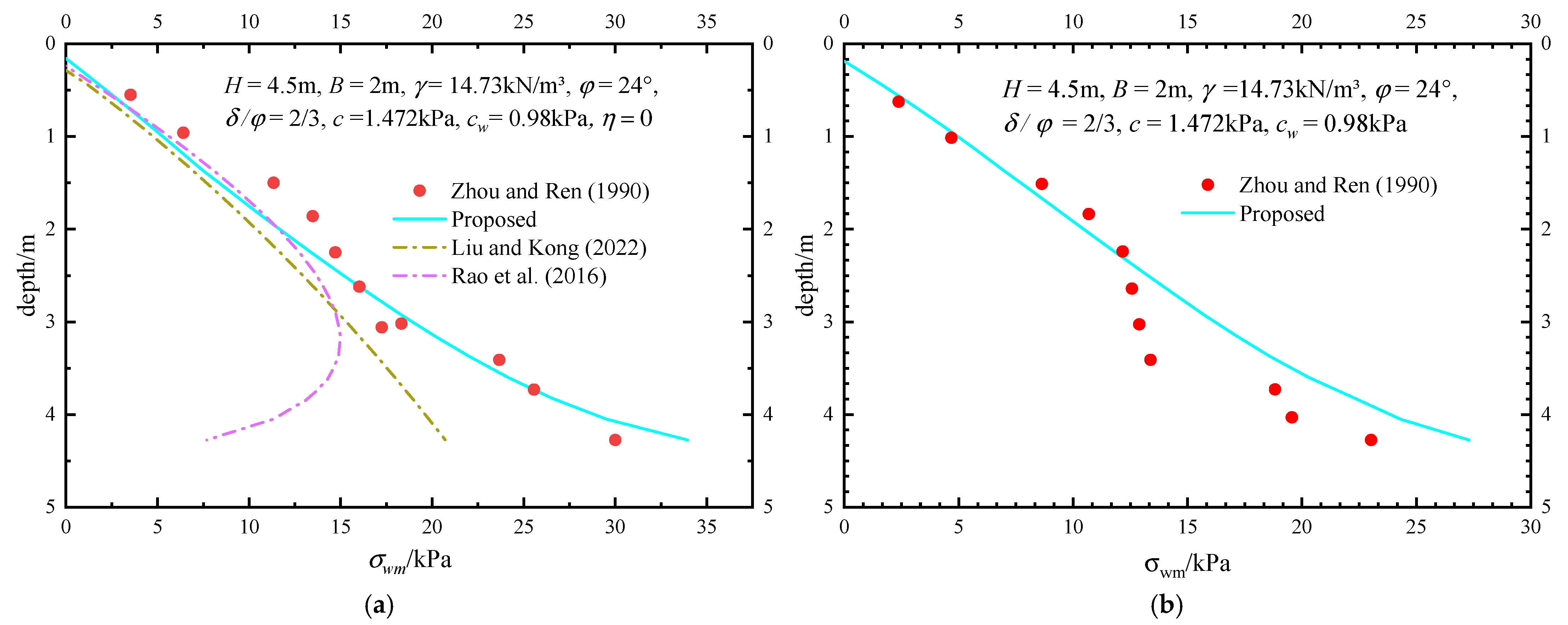
5. Verification by Comparison

Zhou and Ren [49] conducted a model test on a finite-width cohesive soil under RB using the following model parameters: retaining wall height H = 4.45 m, soil width B = 2 m, friction angle of the soil $\phi ={24.27}^{\circ }$, wall–soil friction angle $\delta =2/3\phi$, cohesion of the backfill c = 1.472 kPa, wall–soil interface adhesion force c_w = 0.98 kPa, soil weight γ = 14.73 kN/m³, failure ratio Rf = 0.85, and overload on the ground surface q = 0. In the test, the retaining wall was considered to be in a static state; therefore, the displacement ratio was $\eta =0$. As shown in Figure 9a, our method was compared with the horizontal differential element method of Rao, who assumed a semi-infinite space [19], that of Liu, who assumed a finite space for the calculations [50]. Zhou and Ren [49] also conducted an experimental investigation of the distribution of earth pressure for a wall top displacement of 4.01 cm under RB. Under the condition that the other properties of the soil are consistent with those shown in Figure 9a, the critical horizontal displacement of the cohesive soil was found to be S_c = 0.9%H [42]. Then, the displacement ratio η of the retaining wall gradually decreased with the increasing depth of the soil, and the shear strength index of the soil exhibits a developed value. The comparison between the experimental value and the theoretical value using the proposed method is represented in Figure 9b.

Figure 9. Comparisons of the active earth pressures derived using different methods: (a) η = 0 and (b) η ≠ 0. The mentioned references in the figure are Zhou and Ren (1990) [49], Liu and Kong (2022) [50], Rao et al. [19].

As shown in Figure 9a, when the displacement ratio is η = 0, the proposed soil pressure increases monotonically with the soil depth. The theoretical values well match the experimental ones, indicating the rationality of this method. In addition, Rao’s soil pressure prediction curve is in good agreement with Zhou’s experimental value at a depth of 0–2 m, but it begins to shrink at a depth of 2 m and gradually deviates from our experimental value. Liu’s theoretical soil pressure increases monotonously with the soil depth, and the trend is consistent with our experimental values. However, from a depth of approximately 3 m, the fitting accuracy gradually reduces. As presented in Figure 9b, when the displacement ratio is η ≠ 0, the values predicted in our study are in good agreement with the experimental data.

6. Parameter Sensitivity Analysis

In this paper, we elucidate the influence of soil cohesion c, soil friction angle φ, wall–soil friction angle δ and width-to-height ratio B/H of the filling on the distribution of earth pressure and the height of the resultant force application point. The parameters were determined as follows: retaining wall height H = 4.5 m, filling’s width-to-height ratio B/H = 0.3, soil weight γ = 15 kN/m³, soil friction angle $\phi ={24}^{\circ }$, wall–soil friction angle $\delta =2\phi /3$ (without special provisions), soil cohesion c = 1 kPa, wall–soil interface adhesion force $c_{\mathrm{w}}=2c/3$ (without special provisions), damage ratio R_f = 0.85, wall displacement ratio $\eta =1$, and uniform load on the fill surface q = 0. The relevant parameters were calculated according to specific situations.

6.1. Analysis of the Soil Pressure Distribution Parameters

6.1.1. Effect of B/H on the Earth Pressure Distribution

Figure 10 reveals that the active soil pressure gradually increases with the increasing width-to-height ratio of the filling. When B/H is small, the soil pressure increases rapidly with the aspect ratio. However, when B/H is greater than cotβ, the change in the fill width has no effect on the earth pressure strength. Therefore, B/H = cotβ can be distinguished as the critical value of both the semi-infinite-width and finite-width soil. In the RB mode, with the increasing soil depth, the influence of the aspect ratio on the soil pressure distribution becomes more significant. Further, Figure 10 also indicates that the change in the aspect ratio does not affect the depth of the tensioning cracks.

Figure 10. Effect of B/H on the active earth pressure distribution.

6.1.2. Effect of φ on Soil Pressure Distribution

As shown in Figure 11, in this study, we assumed that the soil friction angle φ changes between ${10}^{\circ }$ and ${30}^{\circ }$ with an interval of $5^{\circ }$. Five groups of data were set up to evaluate the influence of the soil friction angle on the earth pressure distribution. Notably, the roughness factor δ/φ of the wall–soil interface was considered to be a fixed value of 2/3 to exclude its influence on the distribution of the soil pressure. As evident from Figure 11, a larger friction angle results in a smaller active earth pressure; this enhances the soil arching effect [12]. This variation can be explained as follows. Under the RB mode, the backfill tends to slide downward relative to the retaining wall. Considering the wall–soil friction, the wall surface exerts an upward frictional force to prevent the backfill from sliding downward, resulting in the deflection of the principal stress and the soil arching effect. The frictional force provides an upward binding force for the backfill, which offsets the gravity of the soil to some degree, and is equivalent to the reduction in the gravitational force on the soil. The wall–soil friction angle δ increases along with soil friction angle φ, which increases the frictional force, leading to the reduction in the earth pressure.

Figure 11. Effect of φ on the active earth pressure distribution.

6.1.3. Effect of c on the Earth Pressure Distribution

Evidently, to maintain the stability of a cohesive soil (c = 10 kPa), the resistance provided by the retaining wall is far less than that required for a cohesionless soil with the same properties [51]. Therefore, it is vital to consider the influence of soil cohesion in the design of retaining structures. Here, we discuss the influence of soil cohesion c and wall–soil cohesion c_w on the soil pressure distribution based on the Mohr–Coulomb criterion. To control the variable, the relationship between the wall–soil interface adhesion force and the soil cohesion is considered to be c_w = 2/3c. As shown in Figure 12, it is clear that with the increasing soil cohesion, the tensile cracks in the soil gradually extend downward, and the soil pressure decreases. Further, the soil pressure distribution along the depth is the same under different soil cohesions. These results indicate that changes in soil cohesion do not affect soil arching strength.

Figure 12. Effect of soil cohesion c on the active earth pressure distribution.

6.2. Analysing the Height of the Soil-Pressure Application Point

6.2.1. Effect of B/H and φ on the Height of the Resultant Point

As shown in Figure 13, when the soil friction angle is the same (δ/φ = 2/3), the height of the soil-pressure resultant point, h_a, reduces gradually with the increasing width–height ratio B/H, and tends to approach the wall base. When B/H is determined, with the increasing friction angle, the value of h_a gradually approaches that of the wall top. These results indicate that an increase in the aspect ratio of the soil and a decrease in the soil friction angle of filling improve the stability of the retaining structure. When B/H $\ge$ cotβ, only a negligible change is observed in h_a with the increasing aspect ratio. This shows that when B/H $\ge$ cotβ, the slip surface of the soil reaches the filling surface, and the finite-width soil between the retaining walls evolves into a semi-infinite-width soil, which is used in the calculation of the soil pressure.

Figure 13. Effect of φ and B/H on the normalized height of the resultant-force application point.

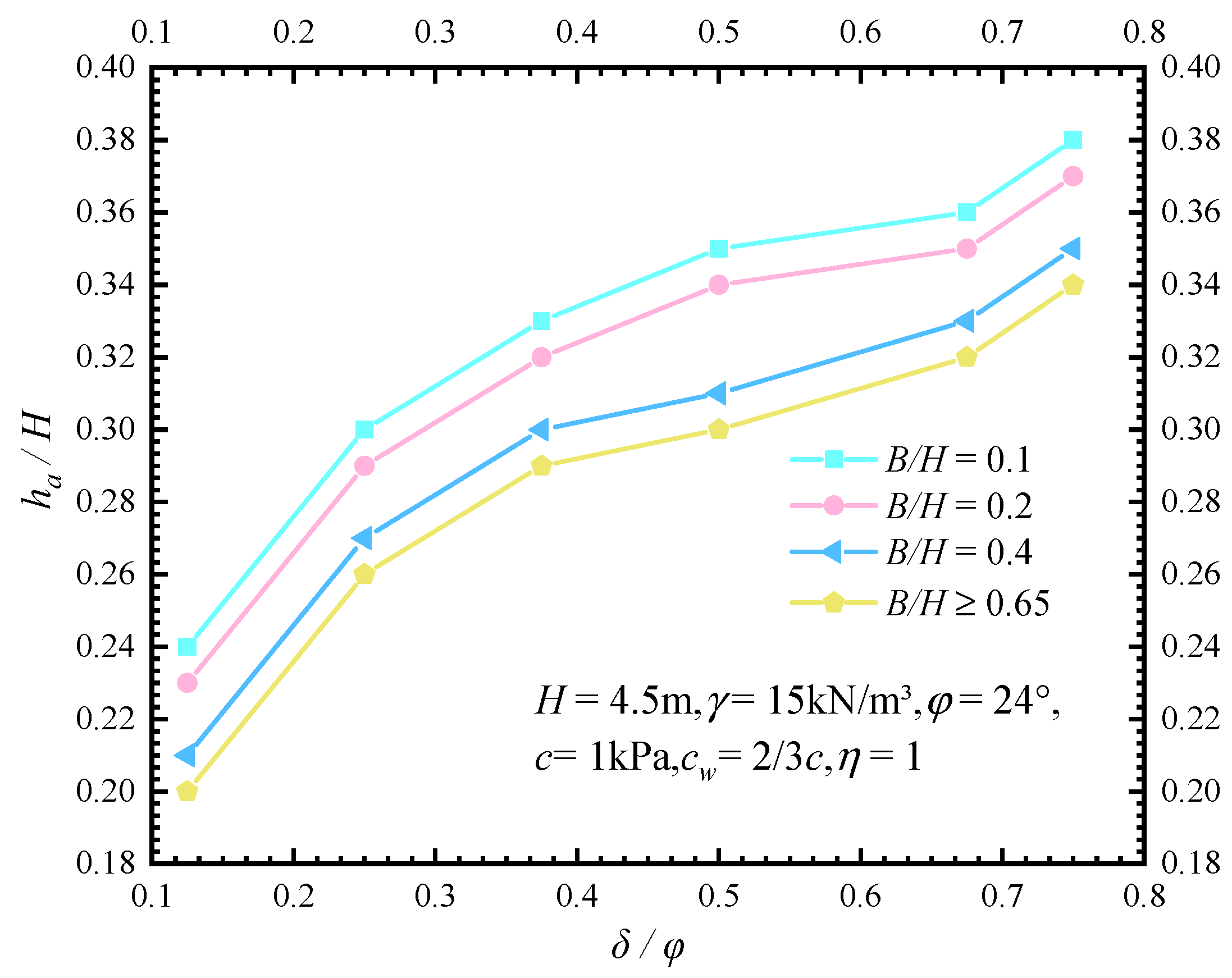
6.2.2. Effect of δ/φ = 2/3 on the Height of the Resultant Point

From Figure 14, it can be observed that for a certain aspect ratio, with an increase in the wall–soil roughness factor (δ/φ), the height of the earth-pressure resultant-force point h_a increases gradually, and the anti-overturn stability of the retaining wall becomes worse. The increase in δ/φ in turn increases the friction force and wall–soil cohesion, as evident from Equations (4) and (5), at the interface of the retaining wall, resulting in a decrease in the earth pressure. However, compared to the soil friction angle φ, the influence of the wall–soil interface roughness factor (δ/φ) on the earth pressure is relatively limited [46].

Figure 14. Effect of δ/φ on the normalized height of the resultant-force application point.

6.2.3. Effect of c on the Height of the Resultant Point

Figure 15 shows that with the increasing soil cohesion c, the height of the resultant-force application point h_a decreases, which is indicative of the soil-cohesion-induced improvement in the anti-overturn stability of the retaining structures. Soil cohesion results in the appearance of tensile cracks with certain depths of the backfill, and the lateral earth pressure in the crack area becomes zero. With an increase in the soil viscosity, the tensile cracks gradually propagate downward to form a larger zone of zero lateral pressure; this causes a downward movement of the application point of the soil-pressure resultant force.

Figure 15. Effect of soil cohesion c on the normalized height of the resultant-force application point.

7. Conclusions

Here, we proposed a new method that includes the effects of soil arching, cohesion and filling width to calculate the active earth pressure under RB. For the calculations, we assumed an approximate slip angle of ${45}^{\circ }+\phi /2$. Based on the results obtained in this study, the following conclusions can be drawn:

(1) Because the wall–soil friction changes the direction of the principal stress transfer, we considered the influence of the soil arching effect in this study to calculate the soil pressure. We simplified the principal stress trace from a circular arc to an inclined line, and the backfill was divided into several inclined thin layers along the inclined line. This effectively avoided the problem of horizontal stress imbalance caused by ignoring the interlayer shear stress in the horizontal differential element method. We proved that this proposed method can improve the calculation accuracy compared to that obtained with the horizontal infinitesimal method.

(2) When the retaining wall is in the nonlimit state, the filling obeys the principle of progressive failure. In addition, the earth pressure is closely related to the displacement of the retaining wall. Thus, to establish the relationship between the shear strength and the wall displacement, we introduced the concepts of displacement ratio η and failure ratio R_f. In this study, the full play value of the shear strength in the earth pressure formula was replaced by the developed value. Thereby, an analytical solution of the nonlimit active earth pressure of a finite-width clay under the RB mode was obtained.

(3) The influence of the width-to-height ratio was considered in the calculation of the earth pressure of a narrow fill. When B/H $\ge$ cotβ, the increasing aspect ratio showed no effect on the earth pressure, because in this case, the filling can be considered as a triangular wedge for the earth pressure calculation. Therefore, B/H = cotβ can be used as the critical value to distinguish between semi-infinite-width and finite-width soil.

(4) For a finite-width soil (B/H < cotβ), a shrinking width–height ratio as well as an increasing friction angle of the soil and soil cohesion contribute to the decrease in the earth pressure. Thus, a reasonable supporting structure can be designed to reduce the earth pressure of the filling by changing these properties of the soil.

(5) For any aspect ratio of the soil, both increasing aspect ratio and soil cohesion as well as decreasing friction angle lower the height of the resultant-force application point, thereby improving the anti-overturning stability of the retaining walls.

This paper can provide a reference for the soil pressure calculation of rotating walls, but it has some limitations. First of all, it assumed an approximate slip angle of ${45}^{\circ }+\phi /2$; thus, further investigations will be conducted for a curved slip surface. Secondly, the study is only for the condition of a unity soil layer; future research needs to consider the earth pressure calculation of layered soils. Last, but not least, this study does not consider the influence of water, and this factor will be added in the next study.

References

- Rankine, W.J.M. On the stability of loose earth. Philos. Trans. R. Soc. Lond. 1857, 147, 9–27. [Google Scholar] [CrossRef] [Green Version]
- Coulomb, C.A. Essai sur Une Application des Règles de Maximis et Minimis Aquelques Problèmes de Statique, Relatifs a l’architecture; Imprimerie Royale; Royal Printing Office: Paris, France, 1776. (In French) [Google Scholar]
- Nian, T.; Han, J. Analytical solution for Rankine’s seismic active earth pressure in c-ϕ soil with infinite slope. J. Geotech. Geoenviron. Eng. 2013, 139, 1611–1616. [Google Scholar] [CrossRef]
- Yang, M.; Dai, X.; Zhao, M.; Luo, H. Experimental study on active earth pressure of cohesionless soil with limited width behind retaining wall. Chin. J. Geotech. Eng. 2016, 38, 131–137. (In Chinese) [Google Scholar]
- Zhang, H.; Liu, M.; Zhou, P.; Zhao, Z.; Li, X.; Xu, X.; Song, X. Analysis of earth pressure variation for partial displacement of retaining wall. Appl. Sci. 2021, 11, 4152. [Google Scholar] [CrossRef]
- Kingsley, H.W. Geostatic wall pressures. Geotech Eng. 1989, 115, 1321–1325. [Google Scholar]
- Yang, T.; He, H.J. Calculation of unlimited passive earth pressure in the model of RBT movement. Adv. Mat. Res. 2011, 250–253, 1572–1577. [Google Scholar] [CrossRef]
- Dou, G.; Xia, J.; Yu, W.; Yuan, F.; Bai, W.G. Nonlimit passive soil pressure on rigid retaining walls. Int. J. Min. Sci. Technol. 2017, 27, 581–587. [Google Scholar] [CrossRef]
- Li, D.; Wang, W.; Zhang, Q. Lateral Earth Pressure behind Walls Rotating about Base considering Arching Effects. Math. Probl. Eng. 2014, 2014, 715891. [Google Scholar] [CrossRef] [Green Version]
- Chen, F.; Lin, Y.; Li, D. Solution to active earth pressure of narrow cohesionless backfill against rigid retaining walls under translation mode. Soils Found. 2018, 59, 151–161. [Google Scholar] [CrossRef]
- Xie, M.; Zheng, J.; Zhang, R.; Cui, L.; Miao, C. Active earth pressure on rigid retaining walls built near rock faces. Int. J. Geomech. 2020, 20, 04020061. [Google Scholar] [CrossRef]
- Terzaghi, K. Theoretical Soil Mechanics; Wiley: New York, NY, USA, 1943; pp. 40–43. [Google Scholar]
- Frydman, S.; Keissar, I. Earth pressure on retaining walls near rock faces. J. Geotech. Eng. 1987, 113, 586–599. [Google Scholar] [CrossRef]
- Tsagareli, Z.V. Experimental investigation of the pressure of a loose medium on re-taining walls with a vertical back face and horizontal backfill surface. Soil Mech. Found. Eng. 1965, 2, 197–200. [Google Scholar] [CrossRef]
- James, R.G.; Bransby, P.L. Experimental and theoretical investigations of a passive earth pressure problem. Geotechnique 1970, 20, 17–37. [Google Scholar] [CrossRef]
- Yang, X.L.; Zhang, S. Seismic active earth pressure for soils with tension cracks. Int. J. Geomech. 2019, 19, 06019009. [Google Scholar] [CrossRef]
- Yang, M.; Tang, X. Rigid retaining walls with narrow cohesionless backfills under various wall movement modes. Int. J. Geomech. 2017, 17, 04017098. [Google Scholar] [CrossRef]
- Goel, S.; Patra, N.R. Effect of arching on active earth pressure for rigid retaining walls considering translation mode. Int. J. Geomech. 2008, 8, 123–133. [Google Scholar] [CrossRef]
- Rao, P.; Chen, Q.; Zhou, Y.; Nimbalkar, S.; Chiaro, G. Determination of active earth pressure on rigid retaining wall considering arching effect in cohesive backfill soil. Int. J. Geomech. 2016, 16, 04015082. [Google Scholar] [CrossRef]
- Cai, Y.; Chen, Q.; Zhou, Y.; Nimbalkar, S.; Yu, J. Estimation of passive earth pressure against rigid retaining wall considering arching effect in cohesive-frictional backfill under translation mode. Int. J. Geomech. 2017, 17, 04016093. [Google Scholar] [CrossRef]
- Pain, A.; Chen, Q.; Nimbalkar, S.; Zhou, Y. Evaluation of seismic passive earth pressure of inclined rigid retaining wall considering soil arching effect. Soil Dyn. Earthq. Eng. 2017, 100, 286–295. [Google Scholar] [CrossRef]
- Zhou, Y.T. Active earth pressure against rigid retaining wall considering effects of wall-soil friction and inclinations. KSCE J. Civ. Eng. 2018, 22, 4901–4908. [Google Scholar] [CrossRef]
- Cao, H.Y.; Liu, J.F.; Wu, C.F.; Du, L. Active earth pressures and tensile crack of the fill in a Nonlimit State. China J. Highw. Transp. 2020, 33, 51–62. (In Chinese) [Google Scholar] [CrossRef]
- Fang, Y.; Ishibashi, I. Static earth pressures with various wall movements. Geotech. Eng. 1986, 112, 317–333. [Google Scholar] [CrossRef]
- Chang, M.F. Lateral earth pressures behind rotating walls. Can. Geotech. J. 1997, 34, 498–509. [Google Scholar] [CrossRef]
- Greco, V. Active thrust on retaining walls of narrow backfill width. Comput. Geotech. 2013, 50, 66–78. [Google Scholar] [CrossRef]
- Lin, Y.-J.; Chen, F.-Q.; Yang, J.-T.; Li, D. Active earth pressure of narrow cohesionless backfill on inclined rigid retaining walls rotating about the bottom. Int. J. Geomech. 2020, 20, 04020102. [Google Scholar] [CrossRef]
- Cao, W.; Zhang, H.; Liu, T.; Tan, X. Analytical solution for the active earth pressure of cohesionless soil behind an inclined retaining wall based on the curved thin-layer element method. Comput. Geotech. 2020, 128, 103851. [Google Scholar] [CrossRef]
- Cao, W.; Liu, T.; Xu, Z. Estimation of active earth pressure on inclined retaining wall based on simplified principal stress trajectory method. Int. J. Geomech. 2019, 19, 06019011. [Google Scholar] [CrossRef]
- Matsuo, M.; Kenmochi, S.; Yagi, H. Experimental study on earth pressure of retaining wall by field tests. Soils Found. 1978, 18, 27–41. [Google Scholar] [CrossRef]
- Gong, C.; Yu, J.; Xu, R.; Wei, G. Calculation of earth pressure against rigid retaining wall rotating outward about base. J. -Zhejiang Univ. Eng. Sci. 2005, 39, 1690–1694. (In Chinese) [Google Scholar]
- Bang, S.C. Active earth pressure behind retaining walls. J. Geotech. Eng. 1985, 111, 407–412. [Google Scholar] [CrossRef]
- Niedostatkiewicz, M.; Lesniewska, D.; Tejchman, J. Experimental Analysis of Shear Zone Patterns in Cohesionless for Earth Pressure Problems Using Particle Image Velocimetry. Strain 2011, 47, 218–231. [Google Scholar] [CrossRef]
- Bourgeois, E.; Soyez, L.; Kouby, A.L. Experimental and numerical study of the behavior of a reinforced-earth wall subjected to a local load. Comput. Geotech. 2011, 38, 515–525. [Google Scholar] [CrossRef]
- Hu, J.; Zhang, Y.; Chen, L. Study on active earth pressure on retaining wall in nonlimit state. Chin. J. Geotech. Eng. 2013, 35, 381–387. (In Chinese) [Google Scholar]
- Sherif, M.; Fang, Y.; Sheriffri, R.I. Ka and Ko behind rotating and non-yielding walls. J. Geotech. Eng. 1984, 110, 41–56. [Google Scholar] [CrossRef]
- Xu, R.Q. Methods of earth pressure calculation for excavation. J. Zhejiang Univ. Eng. Sci. 2000, 34, 370–375. (In Chinese) [Google Scholar]
- Matsuzawa, H.; Hararika, H. Analyses of active earth pressure against rigid retaining walls subjected to different modes of movement. Soils Found. 1996, 36, 51–65. [Google Scholar] [CrossRef] [Green Version]
- Naikai, T. Finite element computations for active and passive earth pressure problems of retaining wall. Soils Found. 1985, 25, 98–112. [Google Scholar] [CrossRef] [Green Version]
- Xu, R.; Liao, B.; Wu, J.; Chang, S. Computational method for active earth pressure of cohesive under nonlimit state. Rock Soil Mech. 2013, 34, 148–154. (In Chinese) [Google Scholar]
- Qian, J.; Yin, Z.Z. Geotechnical Principle and Calculation; Water & Power Press: Beijing, China, 1996. [Google Scholar]
- Liu, J.; Hou, X.Y. Foundation Pit Engineering Manual; China Architecture and Building Press: Beijing, China, 1977. (In Chinese) [Google Scholar]
- Zhao, H.H. A calculation of earth pressure of cohesive fill behind retaining wall. Chin. J. Geotech. Eng. 1983, 5, 134–146. (In Chinese) [Google Scholar]
- Xu, R.; Xu, Y.; Cheng, K.; Feng, S.; Shen, S. Method to calculate active earth pressure considering soil arching effect under nonlimit state of clay. Chin. J. Geotech. Eng. 2020, 42, 362–371. (In Chinese) [Google Scholar]
- Smita, P.; Kousik, D. Study of Active Earth Pressure behind a Vertical Retaining Wall Subjected to Rotation about the Base. Int. J. Geomech. 2020, 20, 04020028. [Google Scholar] [CrossRef]
- Lai, F.; Yang, D.; Liu, S.; Zhang, H.; Cheng, Y. Towards an improved analytical framework to estimate active earth pressure in narrow c–ϕ soils behind rotating walls about the base. Comput. Geotech. 2022, 141, 1–16. [Google Scholar] [CrossRef]
- Yang, D.; Lai, F.; Liu, S.Y. Earth pressure in narrow cohesive-frictional soils behind retaining walls rotated about the top: An analytical approach. Comput. Geotech. 2022, 149, 104849. [Google Scholar] [CrossRef]
- Chen, F.-Q.; Lin, C.; Lin, L.-B.; Huang, M. Active earth pressure of narrow cohesive backfill on rigid retaining wall of rotation about the bottom. Soils Found. 2021, 61, 95–112. [Google Scholar] [CrossRef]
- Zhou, Y.; Ren, M.L. An experimental study on active earth pressure behind rigid retaining wall. Chin. J. Geotech. Eng. 1990, 12, 19–26. (In Chinese) [Google Scholar]
- Liu, H.; Kong, D.Z. Active Earth Pressure of Finite Width Soil Considering Intermediate Principal Stress and Soil Arching Effects. Int. J. Geomech. 2022, 22, 04021294. [Google Scholar] [CrossRef]
- Anderson, D.G. Seismic Analysis and Design of Retaining Walls, Buried Structures, Slopes and Embankments; Transportation Research Board: Washington, DC, USA, 2009. [Google Scholar]
Publisher’s Note: MDPI stays neutral with regard to jurisdictional claims in published maps and institutional affiliations. |
© 2022 by the authors. Licensee MDPI, Basel, Switzerland. This article is an open access article distributed under the terms and conditions of the Creative Commons Attribution (CC BY) license (https://creativecommons.org/licenses/by/4.0/).
Share and Cite
Wang, Z.; Liu, X.; Wang, W.; Tao, Z.; Li, S. Inclined Layer Method-Based Theoretical Calculation of Active Earth Pressure of a Finite-Width Soil for a Rotating-Base Retaining Wall. Sustainability 2022, 14, 9772. https://doi.org/10.3390/su14159772
Wang Z, Liu X, Wang W, Tao Z, Li S. Inclined Layer Method-Based Theoretical Calculation of Active Earth Pressure of a Finite-Width Soil for a Rotating-Base Retaining Wall. Sustainability. 2022; 14(15):9772. https://doi.org/10.3390/su14159772
Chicago/Turabian StyleWang, Zeyue, Xinxi Liu, Weiwei Wang, Ziyu Tao, and Song Li. 2022. "Inclined Layer Method-Based Theoretical Calculation of Active Earth Pressure of a Finite-Width Soil for a Rotating-Base Retaining Wall" Sustainability 14, no. 15: 9772. https://doi.org/10.3390/su14159772
APA StyleWang, Z., Liu, X., Wang, W., Tao, Z., & Li, S. (2022). Inclined Layer Method-Based Theoretical Calculation of Active Earth Pressure of a Finite-Width Soil for a Rotating-Base Retaining Wall. Sustainability, 14(15), 9772. https://doi.org/10.3390/su14159772