
MSSA-DEED: A Multi-Objective Salp Swarm Algorithm for Solving Dynamic Economic Emission Dispatch Problems


Abstract
:1. Introduction
- Proposing the MSSA to find the optimal solution of the non-linear and non-convex multi-objective DEED problems.
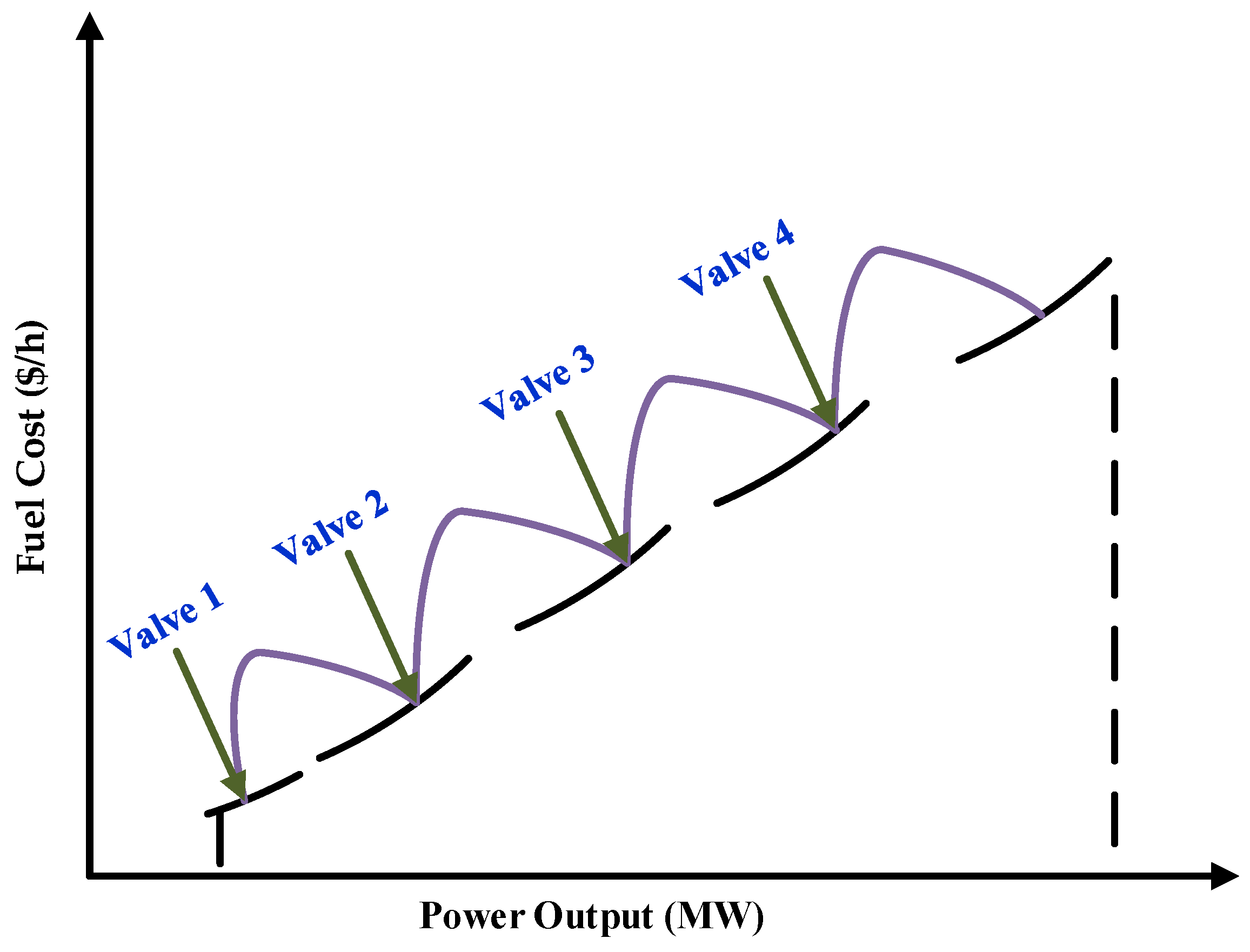
- Solving multi-objective DEED problems considering the valve point effect, transmission loss, as well as the ramping rate.
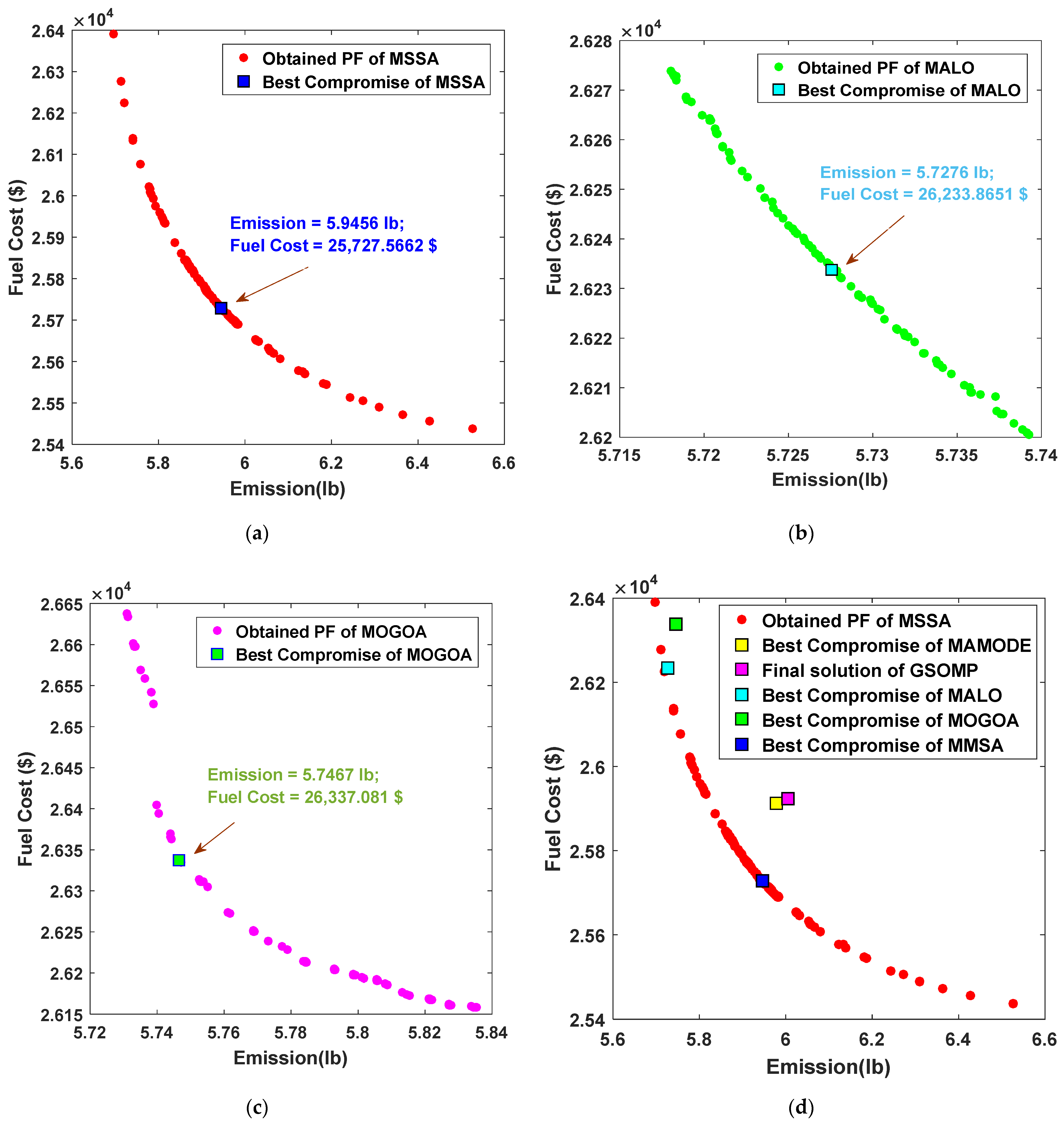
- Applying the fuzzy decision-making approach to achieve the best compromise solutions.
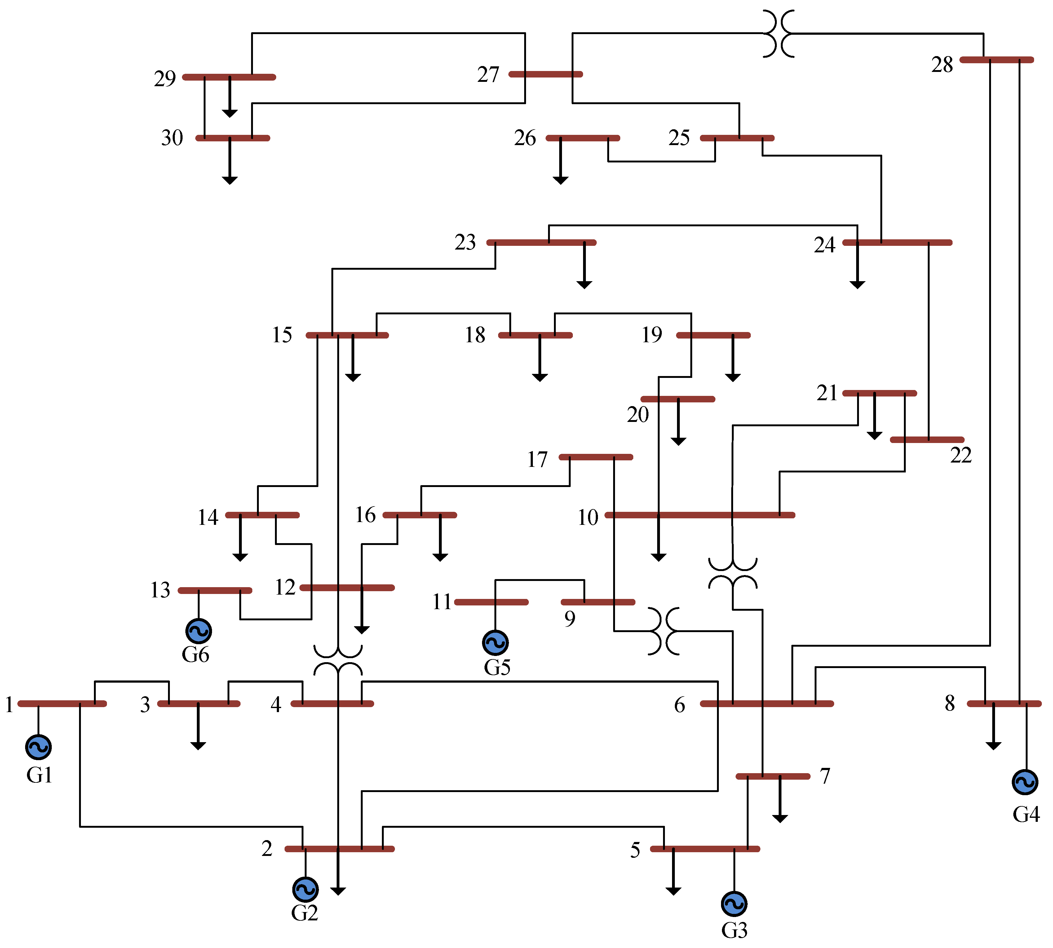
- Using the 6-unit power system, 10-unit power system, and 14-unit power system as three studied cases to prove the efficacy of the MSSA.
2. Mathematical Model of EED Problem
2.1. Objective Functions
2.2. Operational Constraints
2.2.1. Power Balance Constraint
2.2.2. Generating Capacity Constraint
2.2.3. Ramp Rate Constraint
3. Multi-Objective Optimization Algorithm
3.1. Multi-Objective Optimization Problem
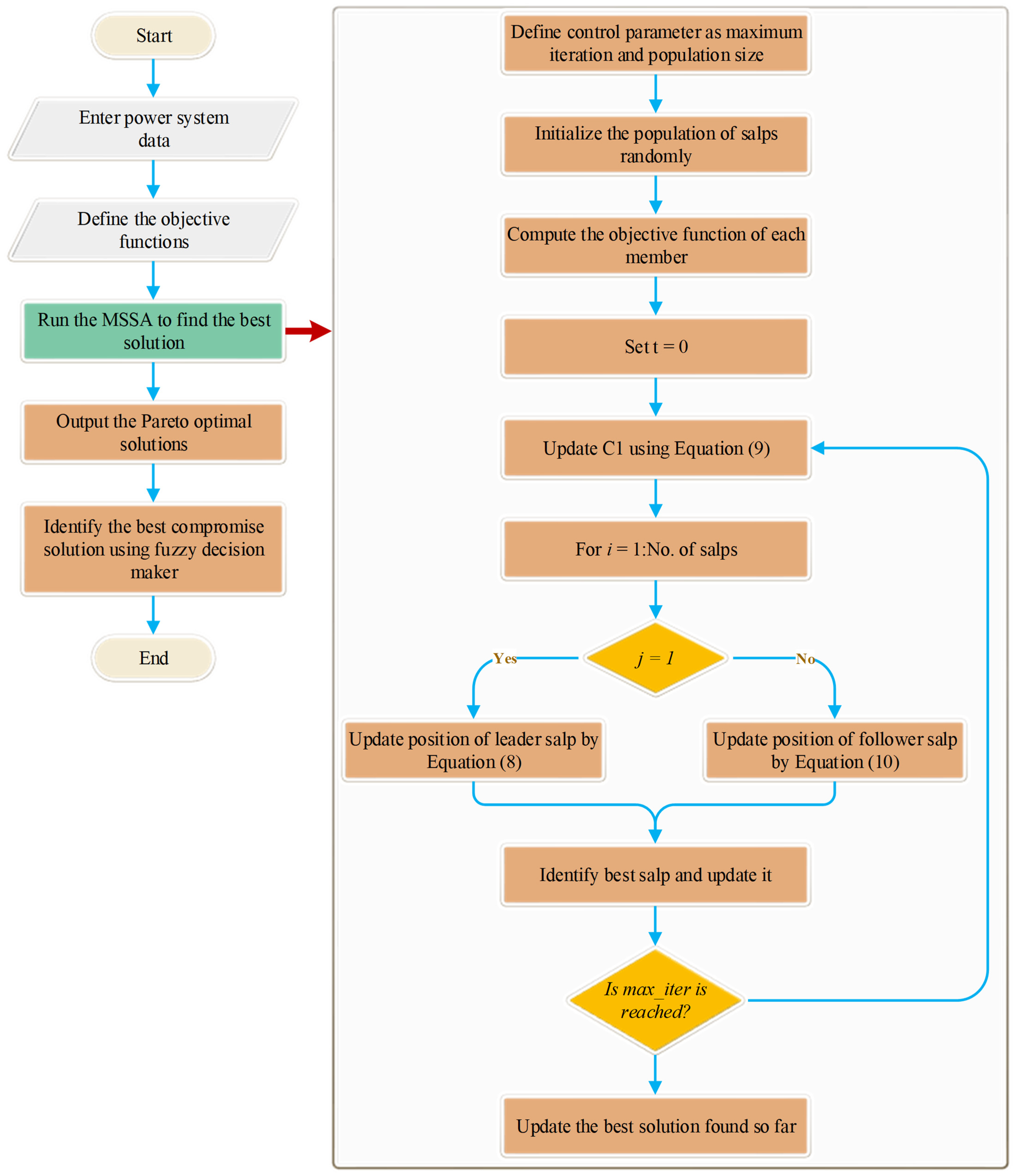
3.2. Multi-Objective Salp Swarm Algorithm
| Algorithm 1 Pseudo code of MSSA |
| Initialize the parameters the number of salps, Obj_no, dim, lb, ub, Archive Maxsize, Initialize the salp population Define the objective function (Dynamic Economic Emission Dispatch function) While Evaluate the fitness of all salp with Ob_func; Find the ND solutions Update the repository in regard to the achieved ND agents If (repository is full); Perform the repository maintenance process to eliminate one repository neighborhood Insert the ND agent to the repository End If Select a source of food from repository Update by Equation (9); For each search agent If (i==1) Update the location of the leading salp by Equation (8); Else Update the location of the leading salp by Equation (10); End if End For End While Return repository |
4. Simulation Results and Discussions
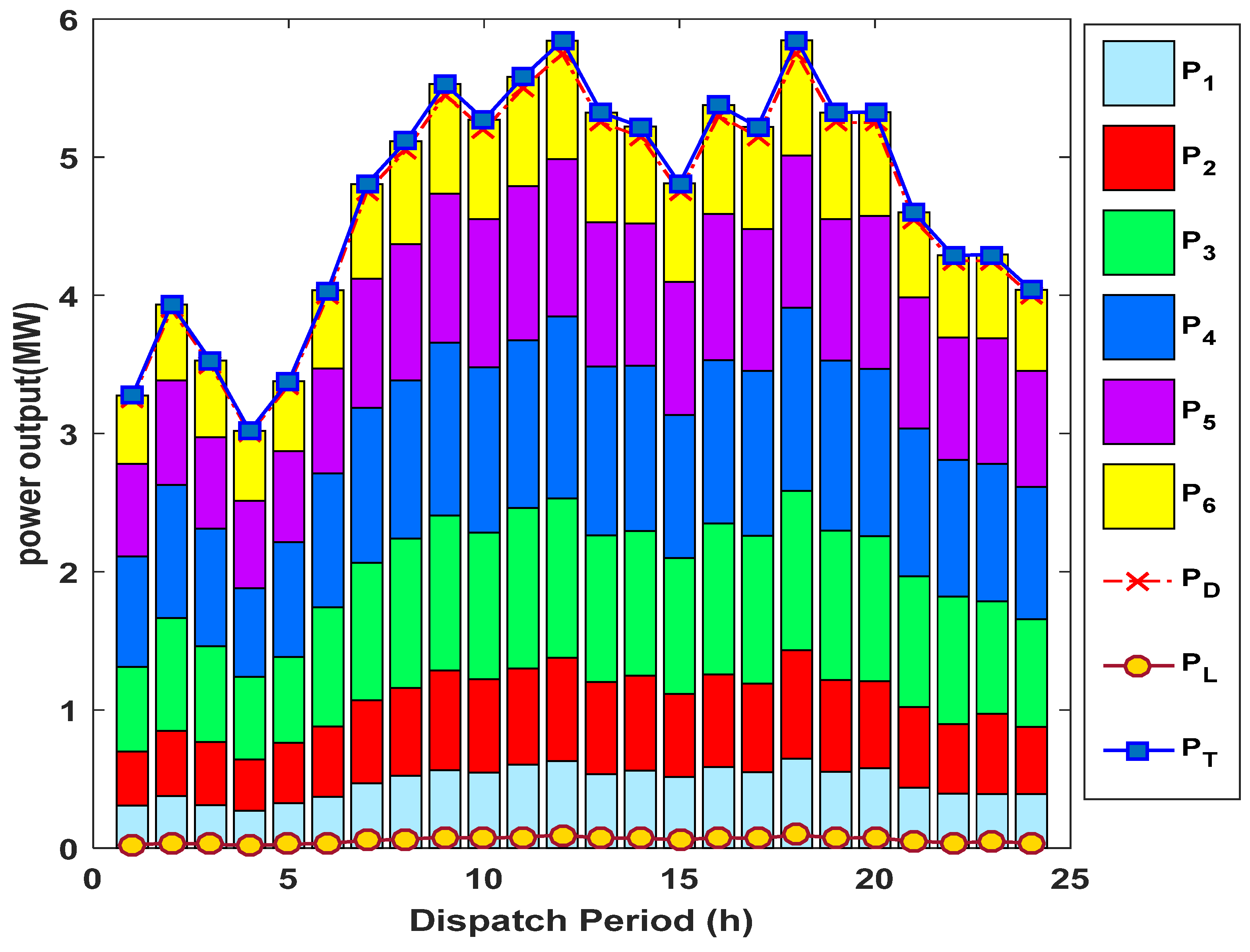
4.1. Case 1: Six-Unit Test System
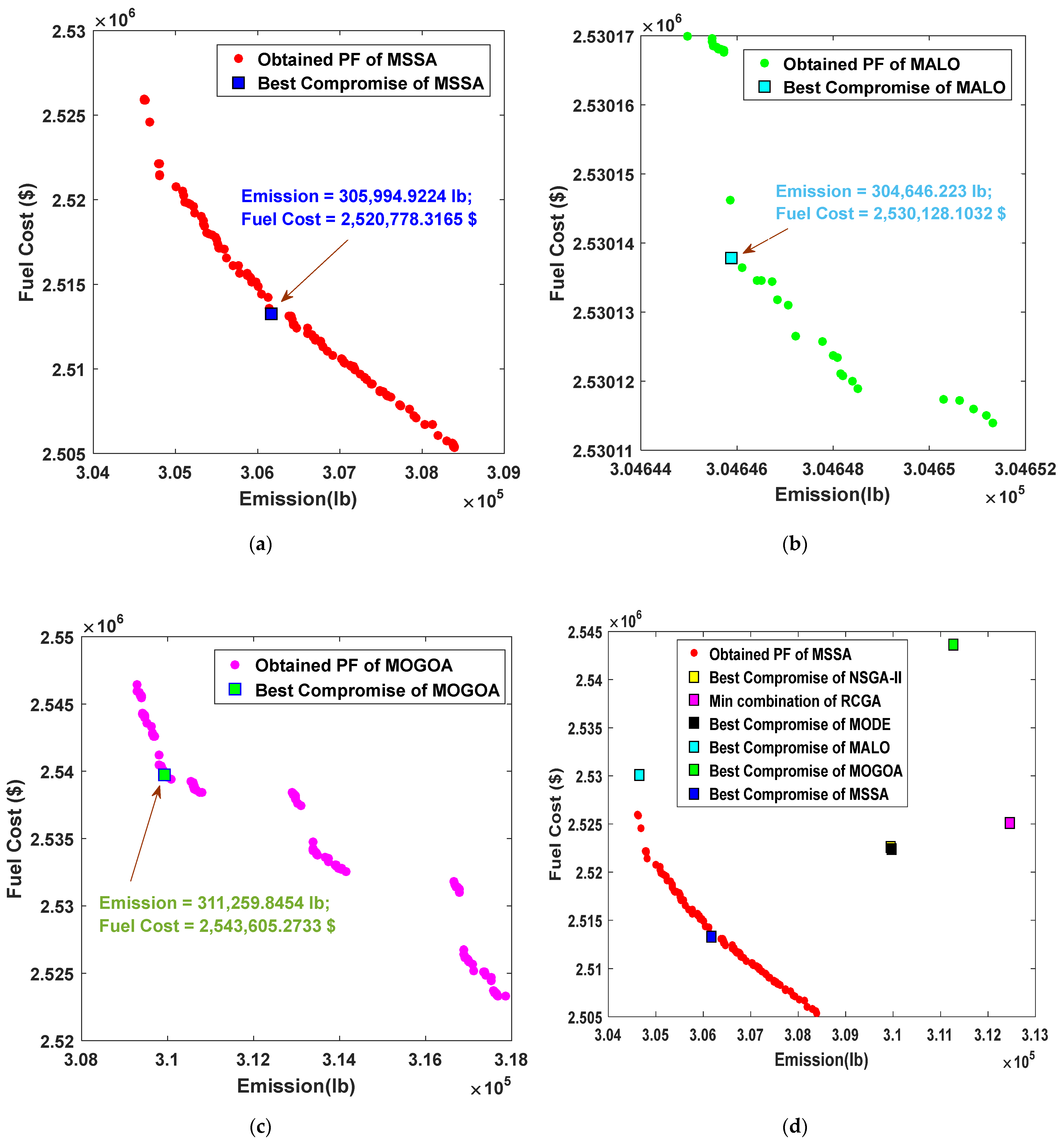
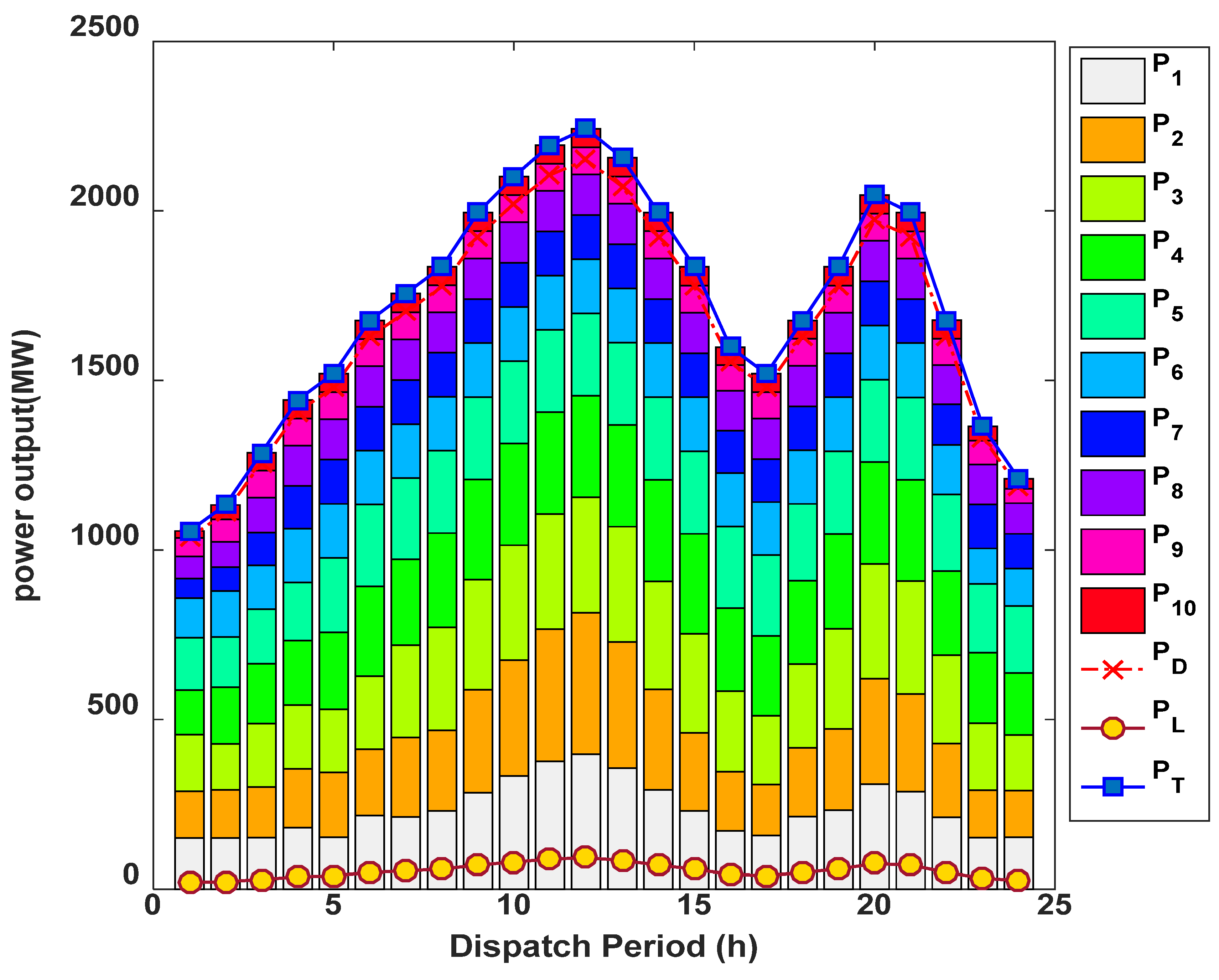
4.2. Case 2: 10-Unit Test System
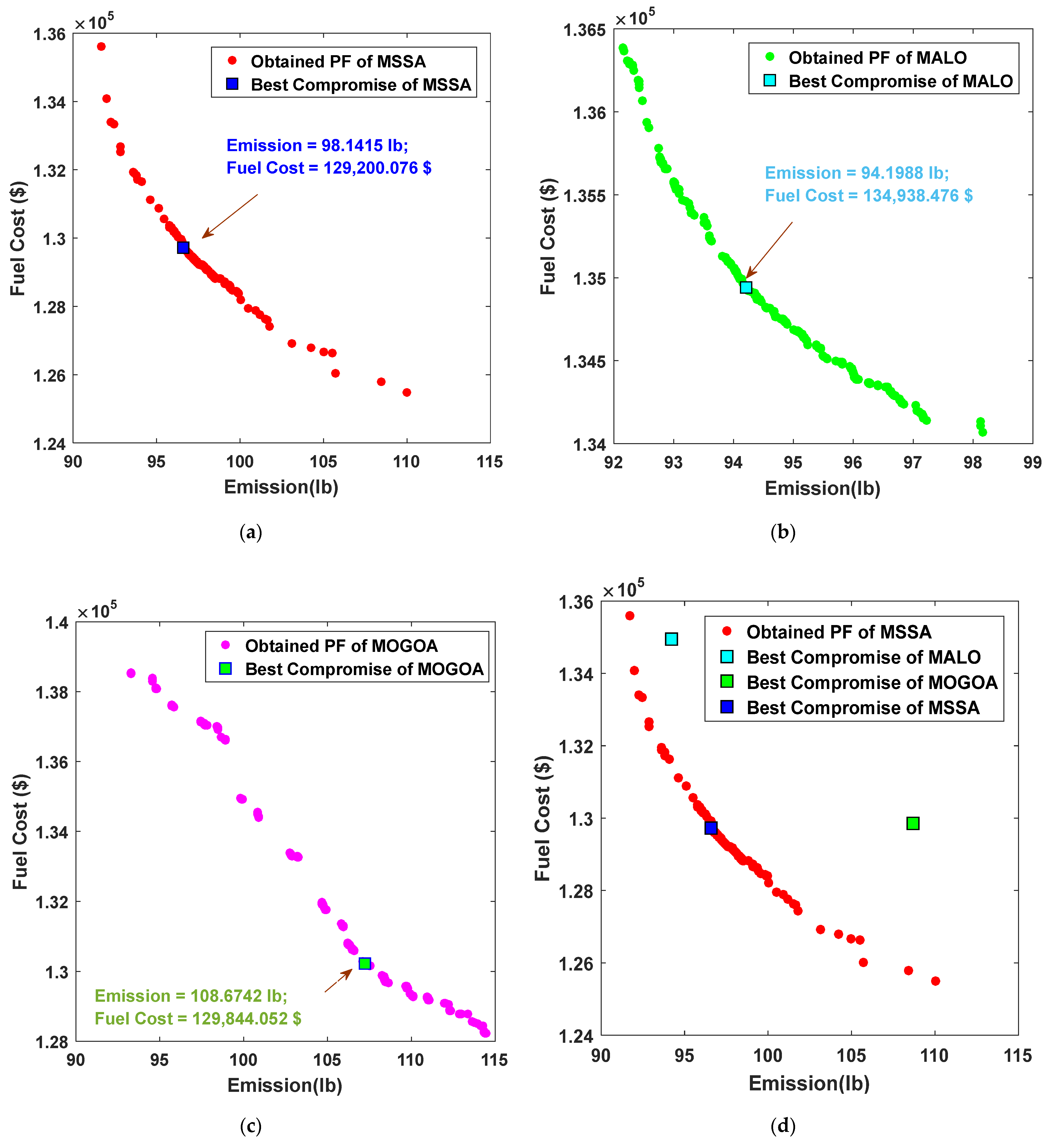
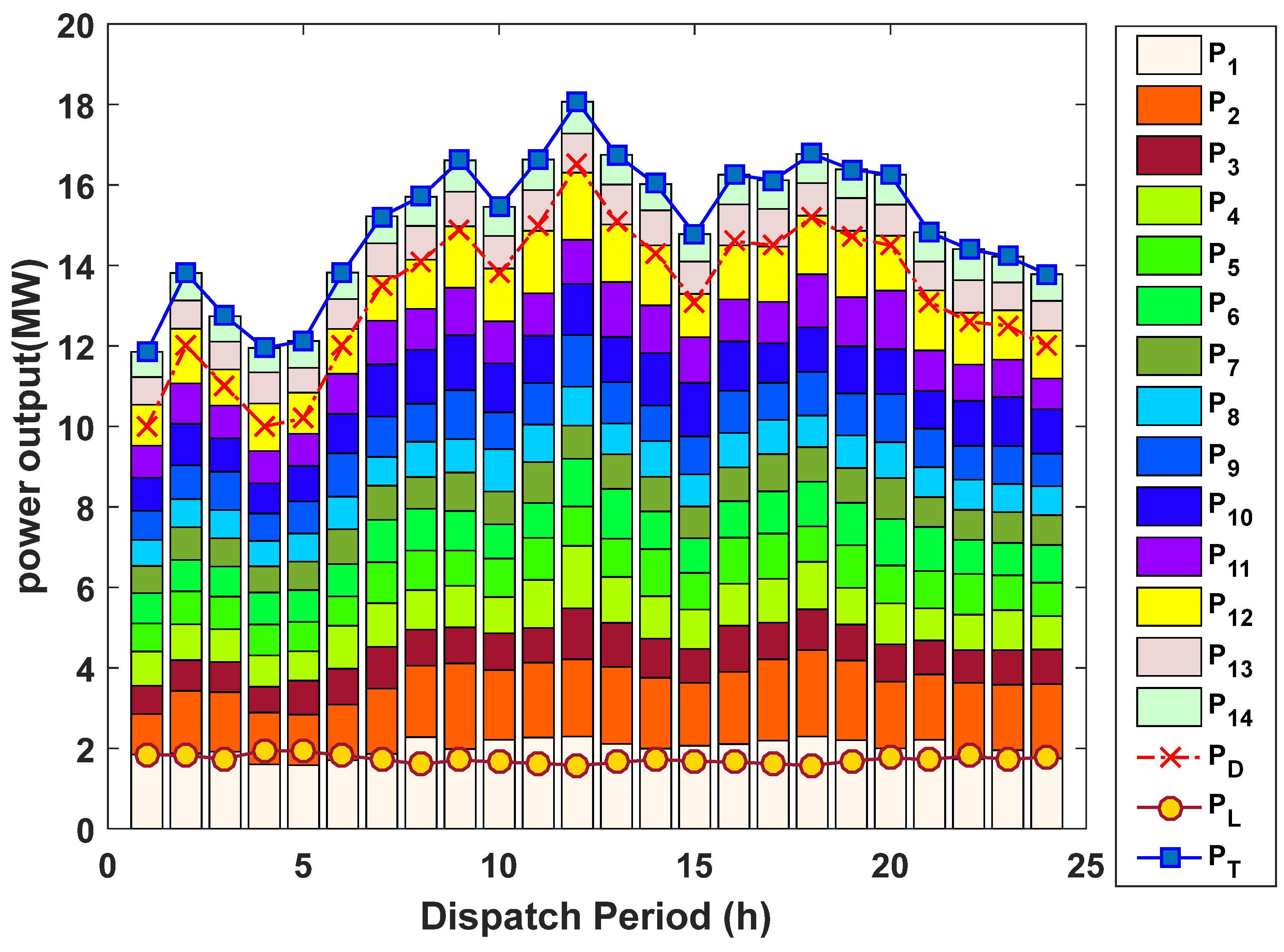
4.3. Case 3: 14-Unit Test System
5. Conclusions
Author Contributions
Funding
Institutional Review Board Statement
Informed Consent Statement
Data Availability Statement
Acknowledgments
Conflicts of Interest
Abbreviations
| DEED | Dynamic Economic and Emission Dispatch |
| FDM | Fuzzy decision-making |
| MSSA | Multi-objective Salp Swarm Algorithm |
| ITSA | Improved tunicate swarm algorithm |
| MALO | Multi-objective ant lion optimizer |
| MOGOA | Multi-objective grasshopper optimization algorithm |
| EED | Economic and Emission Dispatch |
| SSA | Salp Swarm Algorithm |
| ODEA | The opposition-based differential evolution algorithm |
| PSO | Particle swarm optimizer |
| MODE | Multi-objective Differential Evolution |
| CRO | Chemical Reaction Optimization |
| SQP | Sequential quadratic programming |
| EPFSA | Evolutionary programming-based fuzzy satisfying algorithm |
| ELD | Economic Load Dispatch |
| ND | Non-dominated |
| BCS | Best Compromise Solutions |
| VPE | Valve point effect |
| NSGA-II | Non-dominated Sorting Genetic Algorithm-II |
| MOP | Multi-objective optimization problem |
| DED | Dynamic Economic Dispatch |
| IBFA | Improved bacterial foraging algorithm |
| PSOCS | Particle swarm optimization algorithm with a clone selection |
| DE | Differential evolution |
| MAMODE | Modified Adaptive Multi-objective Differential Evolution |
| GSOMP | Group Search Optimizer with Multiple Producers |
| RWS | Roulette wheel selection |
| MONNDE | Multi-objective Neural Networks trained using Differential Evolution |
Appendix A

| Hour | PD | Hour | PD | Hour | PD |
|---|---|---|---|---|---|
| 1 | 3.25 | 9 | 5.45 | 17 | 5.15 |
| 2 | 3.90 | 10 | 5.20 | 18 | 5.75 |
| 3 | 3.50 | 11 | 5.50 | 19 | 5.25 |
| 4 | 3.00 | 12 | 5.75 | 20 | 5.25 |
| 5 | 3.35 | 13 | 5.25 | 21 | 4.55 |
| 6 | 4.00 | 14 | 5.15 | 22 | 4.25 |
| 7 | 4.75 | 15 | 4.75 | 23 | 4.25 |
| 8 | 5.05 | 16 | 5.30 | 24 | 4.00 |
| Unit | ||||||||||
|---|---|---|---|---|---|---|---|---|---|---|
| PG1 | 150 | 5 | 10 | 200 | 100 | 4.091 | −5.543 | 6.49 | 2.00 × 10⁻⁴ | 2.857 |
| PG2 | 150 | 5 | 10 | 150 | 120 | 2.543 | −6.047 | 5.638 | 5.00 × 10⁻⁴ | 3.333 |
| PG3 | 150 | 5 | 20 | 180 | 40 | 4.258 | −5.094 | 4.586 | 1.00 × 10⁻⁶ | 8 |
| PG4 | 150 | 5 | 10 | 100 | 60 | 5.326 | −3.55 | 3.38 | 2.00 × 10⁻³ | 2 |
| PG5 | 150 | 5 | 20 | 180 | 40 | 4.258 | −5.094 | 4.586 | 1.00 × 10⁻⁶ | 8 |
| PG6 | 150 | 5 | 10 | 150 | 100 | 6.131 | −5.555 | 5.151 | 1.00 × 10⁻⁵ | 6.667 |
Appendix B
| Hour | PD | Hour | PD | Hour | PD |
|---|---|---|---|---|---|
| 1 | 1036 | 9 | 1924 | 17 | 1480 |
| 2 | 1110 | 10 | 2022 | 18 | 1628 |
| 3 | 1258 | 11 | 2106 | 19 | 1776 |
| 4 | 1406 | 12 | 2150 | 20 | 1972 |
| 5 | 1480 | 13 | 2072 | 21 | 1924 |
| 6 | 1628 | 14 | 1924 | 22 | 1628 |
| 7 | 1702 | 15 | 1776 | 23 | 1332 |
| 8 | 1776 | 16 | 1554 | 24 | 1184 |
| Unit | |||||||
|---|---|---|---|---|---|---|---|
| PG1 | 150 | 470 | 786.7988 | 38.5379 | 0.1524 | 450 | 0.041 |
| PG2 | 135 | 470 | 451.3251 | 46.1591 | 0.1058 | 600 | 0.036 |
| PG3 | 73 | 340 | 1049.998 | 40.3965 | 0.028 | 320 | 0.028 |
| PG4 | 60 | 300 | 1243.531 | 38.3055 | 0.0354 | 260 | 0.052 |
| PG5 | 73 | 243 | 1658.57 | 36.3278 | 0.0211 | 280 | 0.063 |
| PG6 | 57 | 160 | 1356.659 | 38.2704 | 0.0179 | 310 | 0.048 |
| PG7 | 20 | 130 | 1450.705 | 36.5104 | 0.0121 | 300 | 0.086 |
| PG8 | 47 | 120 | 1450.705 | 36.5104 | 0.0121 | 340 | 0.082 |
| PG9 | 20 | 80 | 1455.606 | 39.5804 | 0.109 | 270 | 0.098 |
| PG10 | 10 | 55 | 1469.403 | 40.5407 | 0.1295 | 380 | 0.094 |
| Unit | |||||||
|---|---|---|---|---|---|---|---|
| P1 | 103.3908 | 2.4444 | 0.0312 | 0.5035 | 0.0207 | 80 | 80 |
| P2 | 103.3908 | 2.4444 | 0.0312 | 0.5035 | 0.0207 | 80 | 80 |
| P3 | 300.391 | 4.0695 | 0.0509 | 0.4968 | 0.0202 | 80 | 80 |
| P4 | 300.391 | 4.0695 | 0.0509 | 0.4968 | 0.0202 | 50 | 50 |
| P5 | 320.0006 | 3.8132 | 0.0344 | 0.4972 | 0.02 | 50 | 50 |
| P6 | 320.0006 | 3.8132 | 0.0344 | 0.4972 | 0.02 | 50 | 50 |
| P7 | 330.0056 | 3.9023 | 0.0465 | 0.5163 | 0.0214 | 50 | 30 |
| P8 | 330.0056 | 3.9023 | 0.0465 | 0.5163 | 0.0214 | 30 | 30 |
| P9 | 350.0056 | 3.9524 | 0.0465 | 0.5475 | 0.0234 | 30 | 30 |
| P10 | 360.0012 | 3.9864 | 0.047 | 0.5475 | 0.0234 | 30 | 30 |
| 0.000049 | 0.000014 | 0.000015 | 0.000015 | 0.000016 | 0.000017 | 0.000017 | 0.000018 | 0.000019 | 0.00002 | |
|---|---|---|---|---|---|---|---|---|---|---|
| 0.000014 | 0.000045 | 0.000016 | 0.000016 | 0.000017 | 0.000015 | 0.000015 | 0.000016 | 0.000018 | 0.000018 | |
| 0.000015 | 0.000016 | 0.000039 | 0.00001 | 0.000012 | 0.000012 | 0.000014 | 0.000014 | 0.000016 | 0.000016 | |
| 0.000015 | 0.000016 | 0.00001 | 0.00004 | 0.000014 | 0.00001 | 0.000011 | 0.000012 | 0.000014 | 0.000015 | |
| 0.000016 | 0.000017 | 0.000012 | 0.000014 | 0.000035 | 0.000011 | 0.000013 | 0.000013 | 0.000015 | 0.000016 | |
| 0.000017 | 0.000015 | 0.000012 | 0.00001 | 0.000011 | 0.000036 | 0.000012 | 0.000012 | 0.000014 | 0.000015 | |
| 0.000017 | 0.000015 | 0.000014 | 0.000011 | 0.000013 | 0.000012 | 0.000038 | 0.000016 | 0.000016 | 0.000018 | |
| 0.000018 | 0.000016 | 0.000014 | 0.000012 | 0.000013 | 0.000012 | 0.000016 | 0.00004 | 0.000015 | 0.000016 | |
| 0.000019 | 0.000018 | 0.000016 | 0.000014 | 0.000015 | 0.000014 | 0.000016 | 0.000015 | 0.000042 | 0.000019 | |
| 0.00002 | 0.000018 | 0.000016 | 0.000015 | 0.00016 | 0.000015 | 0.000018 | 0.000016 | 0.000019 | 0.000044 | |
| 0 | 0 | 0 | 0 | 0 | 0 | 0 | 0 | 0 | 0 | |
| 0 |
Appendix C
| Hour | PD | Hour | PD | Hour | PD |
|---|---|---|---|---|---|
| 1 | 10.0 | 9 | 14.9 | 17 | 14.5 |
| 2 | 12.0 | 10 | 13.8 | 18 | 15.2 |
| 3 | 11.0 | 11 | 15.0 | 19 | 14.7 |
| 4 | 10.0 | 12 | 16.5 | 20 | 14.5 |
| 5 | 10.2 | 13 | 15.1 | 21 | 13.1 |
| 6 | 12.0 | 14 | 14.3 | 22 | 12.6 |
| 7 | 13.5 | 15 | 13.1 | 23 | 12.5 |
| 8 | 14.1 | 16 | 14.6 | 24 | 12.0 |
| Unit | ||||||||
|---|---|---|---|---|---|---|---|---|
| PG1 | 300 | 50 | 150 | 189 | 0.5 | 0.016 | −1.5 | 23.333 |
| PG2 | 300 | 50 | 115 | 200 | 0.55 | 0.031 | −1.82 | 21.022 |
| PG3 | 300 | 50 | 40 | 350 | 0.6 | 0.013 | −1.249 | 22.05 |
| PG4 | 300 | 50 | 122 | 315 | 0.5 | 0.012 | −1.355 | 22.983 |
| PG5 | 300 | 50 | 125 | 305 | 0.5 | 0.02 | −1.9 | 21.313 |
| PG6 | 300 | 50 | 70 | 275 | 0.7 | 0.007 | 0.805 | 21.9 |
| PG7 | 300 | 50 | 70 | 345 | 0.7 | 0.015 | −1.401 | 23.001 |
| PG8 | 300 | 50 | 70 | 345 | 0.7 | 0.018 | −1.8 | 24.003 |
| PG9 | 300 | 50 | 130 | 245 | 0.5 | 0.019 | −2 | 25.121 |
| PG10 | 300 | 50 | 130 | 245 | 0.5 | 0.012 | −1.36 | 22.99 |
| PG11 | 300 | 50 | 135 | 235 | 0.55 | 0.033 | −2.1 | 27.01 |
| PG12 | 300 | 50 | 200 | 130 | 0.45 | 0.018 | −1.8 | 25.101 |
| PG13 | 300 | 50 | 70 | 345 | 0.7 | 0.018 | −1.81 | 24.313 |
| PG14 | 300 | 50 | 45 | 389 | 0.6 | 0.03 | −1.921 | 27.119 |
References
- Alomoush, M.I.; Oweis, Z.B. Environmental-Economic Dispatch Using Stochastic Fractal Search Algorithm. Int. Trans. Electr. Energy Syst. 2018, 28, e2530. [Google Scholar] [CrossRef]
- Edwin Selva Rex, C.R.; Beno, M.M.; Annrose, J. Optimal Power Flow-Based Combined Economic and Emission Dispatch Problems Using Hybrid PSGWO Algorithm. J. Circuits Syst. Comput. 2019, 28, 1950154. [Google Scholar] [CrossRef]
- Talaq, J.H.; El-Hawary, F.; El-Hawary, M.E. A Summary of Environmental/Economic Dispatch Algorithms. IEEE Trans. Power Syst. 1994, 9, 1508–1516. [Google Scholar] [CrossRef]
- Xian, L.; Xu, W. Minimum Emission Dispatch Constrained by Stochastic Wind Power Availability and Cost. IEEE Trans. Power Syst. 2010, 25, 1705–1713. [Google Scholar] [CrossRef]
- Qiao, B.; Zhang, X.; Gao, J.; Liu, R.; Chen, X. Sparse Deconvolution for the Large-Scale Ill-Posed Inverse Problem of Impact Force Reconstruction. Mech. Syst. Signal Process. 2017, 83, 93–115. [Google Scholar] [CrossRef]
- Qu, B.Y.; Zhou, Q.; Xiao, J.M.; Liang, J.J.; Suganthan, P.N. Large-Scale Portfolio Optimization Using Multiobjective Evolutionary Algorithms and Preselection Methods. Math. Probl. Eng. 2017, 2017, 4197914. [Google Scholar] [CrossRef]
- Zou, D.; Li, S.; Li, Z.; Kong, X. A New Global Particle Swarm Optimization for the Economic Emission Dispatch with or without Transmission Losses. Energy Convers. Manag. 2017, 139, 45–70. [Google Scholar] [CrossRef]
- Xia, X.; Elaiw, A.M. Optimal Dynamic Economic Dispatch of Generation: A Review. Electr. Power Syst. Res. 2010, 80, 975–986. [Google Scholar] [CrossRef]
- Mohamed, A.-A.A.; Hassan, S.A.; Hemeida, A.M.; Alkhalaf, S.; Mahmoud, M.M.M.; Eldin, A.M.B. Parasitism–Predation Algorithm (PPA): A Novel Approach for Feature Selection. Ain Shams Eng. J. 2020, 11, 293–308. [Google Scholar] [CrossRef]
- Kamel, S.; Houssein, E.H.; Hassan, M.H.; Shouran, M.; Hashim, F.A. An Efficient Electric Charged Particles Optimization Algorithm for Numerical Optimization and Optimal Estimation of Photovoltaic Models. Mathematics 2022, 10, 913. [Google Scholar] [CrossRef]
- Hassan, M.H.; Kamel, S.; Selim, A.; Khurshaid, T.; Domínguez-García, J.L. A Modified Rao-2 Algorithm for Optimal Power Flow Incorporating Renewable Energy Sources. Mathematics 2021, 9, 1532. [Google Scholar] [CrossRef]
- Mohamed, A.-A.; Al-Jaafary, A.; Mohamed, Y. Optimal Number, Location and Sizing Of FACTS Devices For Optimal Power Flow Using Genetic Algorithm. Aswan Univ. J. Sci. Technol. 2021, 1, 55–73. [Google Scholar]
- Hassan, M.H.; Elsayed, S.K.; Kamel, S.; Rahmann, C.; Taha, I.B.M. Developing Chaotic Bonobo Optimizer for Optimal Power Flow Analysis Considering Stochastic Renewable Energy Resources. Int. J. Energy Res. 2022, 46, 11291–11325. [Google Scholar] [CrossRef]
- Hassan, M.H.; Kamel, S.; El-Dabah, M.A.; Khurshaid, T.; Dominguez-Garcia, J.L. Optimal Reactive Power Dispatch with Time-Varying Demand and Renewable Energy Uncertainty Using Rao-3 Algorithm. IEEE Access 2021, 9, 23264–23283. [Google Scholar] [CrossRef]
- Mirjalili, S.; Gandomi, A.H.; Mirjalili, S.Z.; Saremi, S.; Faris, H.; Mirjalili, S.M. Salp Swarm Algorithm: A Bio-Inspired Optimizer for Engineering Design Problems. Adv. Eng. Softw. 2017, 114, 163–191. [Google Scholar] [CrossRef]
- Granelli, G.P.; Montagna, M.; Pasini, G.L.; Marannino, P. Emission Constrained Dynamic Dispatch. Electr. Power Syst. Res. 1992, 24, 55–64. [Google Scholar] [CrossRef]
- Basu, M. Dynamic Economic Emission Dispatch Using Evolutionary Programming and Fuzzy Satisfying Method. Int. J. Emerg. Electr. Power Syst. 2007, 8, 1. [Google Scholar] [CrossRef]
- Pandit, N.; Tripathi, A.; Tapaswi, S.; Pandit, M. An Improved Bacterial Foraging Algorithm for Combined Static/Dynamic Environmental Economic Dispatch. Appl. Soft Comput. 2012, 12, 3500–3513. [Google Scholar] [CrossRef]
- Benhamida, F.; Belhachem, R. Dynamic Constrained Economic/Emission Dispatch Scheduling Using Neural Network. Adv. Electr. Electron. Eng. 2013, 11, 1. [Google Scholar] [CrossRef]
- Thenmalar, K.; Ramesh, S.; Thiruvenkadam, S. Opposition Based Differential Evolution Algorithm for Dynamic Economic Emission Load Dispatch (EELD) with Emission Constraints and Valve Point Effects. J. Electr. Eng. Technol. 2015, 10, 1508–1517. [Google Scholar] [CrossRef] [Green Version]
- Basu, M. Particle Swarm Optimization Based Goal-Attainment Method for Dynamic Economic Emission Dispatch. Electr. Power Compon. Syst. 2006, 34, 1015–1025. [Google Scholar] [CrossRef]
- Bahmanifirouzi, B.; Farjah, E.; Niknam, T. Multi-Objective Stochastic Dynamic Economic Emission Dispatch Enhancement by Fuzzy Adaptive Modified Theta Particle Swarm Optimization. J. Renew. Sustain. Energy 2012, 4, 023105. [Google Scholar] [CrossRef]
- Elaiw, A.M.; Xia, X.; Shehata, A.M. Hybrid DE-SQP and Hybrid PSO-SQP Methods for Solving Dynamic Economic Emission Dispatch Problem with Valve-Point Effects. Electr. Power Syst. Res. 2013, 103, 192–200. [Google Scholar] [CrossRef]
- Basu, M. Dynamic Economic Emission Dispatch Using Nondominated Sorting Genetic Algorithm-II. Int. J. Electr. Power Energy Syst. 2008, 30, 140–149. [Google Scholar] [CrossRef]
- Basu, M. Multi-Objective Differential Evolution for Dynamic Economic Emission Dispatch. Int. J. Emerg. Electr. Power Syst. 2014, 15, 141–150. [Google Scholar] [CrossRef]
- Jiang, X.; Zhou, J.; Wang, H.; Zhang, Y. Dynamic Environmental Economic Dispatch Using Multiobjective Differential Evolution Algorithm with Expanded Double Selection and Adaptive Random Restart. Int. J. Electr. Power Energy Syst. 2013, 49, 399–407. [Google Scholar] [CrossRef]
- Roy, P.K.; Bhui, S. A Multi-Objective Hybrid Evolutionary Algorithm for Dynamic Economic Emission Load Dispatch. Int. Trans. Electr. Energy Syst. 2016, 26, 49–78. [Google Scholar] [CrossRef]
- Zhu, Z.; Wang, J.; Baloch, M.H. Dynamic Economic Emission Dispatch Using Modified NSGA-II. Int. Trans. Electr. Energy Syst. 2016, 26, 2684–2698. [Google Scholar] [CrossRef]
- Guo, C.X.; Zhan, J.P.; Wu, Q.H. Dynamic Economic Emission Dispatch Based on Group Search Optimizer with Multiple Producers. Electr. Power Syst. Res. 2012, 86, 8–16. [Google Scholar] [CrossRef]
- Li, L.-L.; Liu, Z.-F.; Tseng, M.-L.; Zheng, S.-J.; Lim, M.K. Improved Tunicate Swarm Algorithm: Solving the Dynamic Economic Emission Dispatch Problems. Appl. Soft Comput. 2021, 108, 107504. [Google Scholar] [CrossRef]
- Qian, S.; Wu, H.; Xu, G. An Improved Particle Swarm Optimization with Clone Selection Principle for Dynamic Economic Emission Dispatch. Soft Comput. 2020, 24, 15249–15271. [Google Scholar] [CrossRef]
- Zhang, H.; Yue, D.; Xie, X.; Hu, S.; Weng, S. Multi-Elite Guide Hybrid Differential Evolution with Simulated Annealing Technique for Dynamic Economic Emission Dispatch. Appl. Soft Comput. 2015, 34, 312–323. [Google Scholar] [CrossRef]
- Shao, Z.; Si, F.; Wu, H.; Tong, X. An Agile and Intelligent Dynamic Economic Emission Dispatcher Based on Multi-Objective Proximal Policy Optimization. Appl. Soft Comput. 2021, 102, 107047. [Google Scholar] [CrossRef]
- Mason, K.; Duggan, J.; Howley, E. A Multi-Objective Neural Network Trained with Differential Evolution for Dynamic Economic Emission Dispatch. Int. J. Electr. Power Energy Syst. 2018, 100, 201–221. [Google Scholar] [CrossRef]
- Mirjalili, S.; Jangir, P.; Saremi, S. Multi-Objective Ant Lion Optimizer: A Multi-Objective Optimization Algorithm for Solving Engineering Problems. Appl. Intell. 2017, 46, 79–95. [Google Scholar] [CrossRef]
- Mirjalili, S.Z.; Mirjalili, S.; Saremi, S.; Faris, H.; Aljarah, I. Grasshopper Optimization Algorithm for Multi-Objective Optimization Problems. Appl. Intell. 2018, 48, 805–820. [Google Scholar] [CrossRef]
- Khan, I.U.; Javaid, N.; Gamage, K.A.A.; Taylor, C.J.; Baig, S.; Ma, X. Heuristic Algorithm Based Optimal Power Flow Model Incorporating Stochastic Renewable Energy Sources. IEEE Access 2020, 8, 148622–148643. [Google Scholar] [CrossRef]
- Shen, X.; Zou, D.; Duan, N.; Zhang, Q. An Efficient Fitness-Based Differential Evolution Algorithm and a Constraint Handling Technique for Dynamic Economic Emission Dispatch. Energy 2019, 186, 115801. [Google Scholar] [CrossRef]
- Li, Z.; Zou, D.; Kong, Z. A Harmony Search Variant and a Useful Constraint Handling Method for the Dynamic Economic Emission Dispatch Problems Considering Transmission Loss. Eng. Appl. Artif. Intell. 2019, 84, 18–40. [Google Scholar] [CrossRef]
- Sattar, M.K.; Ahmad, A.; Fayyaz, S.; Ul Haq, S.S.; Saddique, M.S. Ramp Rate Handling Strategies in Dynamic Economic Load Dispatch (DELD) Problem Using Grey Wolf Optimizer (GWO). J. Chin. Inst. Eng. 2020, 43, 200–213. [Google Scholar] [CrossRef]
- Wang, J.; Gao, Y.; Chen, X. A Novel Hybrid Interval Prediction Approach Based on Modified Lower Upper Bound Estimation in Combination with Multi-Objective Salp Swarm Algorithm for Short-Term Load Forecasting. Energies 2018, 11, 1561. [Google Scholar] [CrossRef] [Green Version]
- Hassan, M.H.; Kamel, S.; Abualigah, L.; Eid, A. Development and Application of Slime Mould Algorithm for Optimal Economic Emission Dispatch. Expert Syst. Appl. 2021, 182, 115205. [Google Scholar] [CrossRef]
- Wang, G.; Zha, Y.; Wu, T.; Qiu, J.; Peng, J.; Xu, G. Cross Entropy Optimization Based on Decomposition for Multi-Objective Economic Emission Dispatch Considering Renewable Energy Generation Uncertainties. Energy 2020, 193, 116790. [Google Scholar] [CrossRef]
- Zhu, Y.; Wang, J.; Qu, B. Multi-Objective Economic Emission Dispatch Considering Wind Power Using Evolutionary Algorithm Based on Decomposition. Int. J. Electr. Power Energy Syst. 2014, 63, 434–445. [Google Scholar] [CrossRef]
- Qiao, B.; Liu, J.; Hao, X. A Multi-Objective Differential Evolution Algorithm and a Constraint Handling Mechanism Based on Variables Proportion for Dynamic Economic Emission Dispatch Problems. Appl. Soft Comput. 2021, 108, 107419. [Google Scholar] [CrossRef]
- Wu, L.H.; Wang, Y.N.; Yuan, X.F.; Zhou, S.W. Environmental/Economic Power Dispatch Problem Using Multi-Objective Differential Evolution Algorithm. Electr. Power Syst. Res. 2010, 80, 1171–1181. [Google Scholar] [CrossRef]

| Case Number | Number of Generators | Number of Buses | Number of Decision Variables | Number of Equality Constraints |
|---|---|---|---|---|
| Case 1 | 6 | 30 | 6 × 24 = 144 | 24 |
| Case 2 | 10 | NA | 10 × 24 = 240 | 24 |
| Case 3 | 14 | 118 | 14 × 24 = 336 | 24 |
| Algorithm | Objectives | Total Cost (USD) | Emission (Ib) |
|---|---|---|---|
| MSSA | BC | 25,437.59 | 6.52773 |
| BE | 26,389.76 | 5.69654 | |
| BCS | 25,727.57 | 5.94564 | |
| MALO | BC | 26,200.57 | 5.73927 |
| BE | 26,273.83 | 5.71806 | |
| BCS | 26,233.87 | 5.72757 | |
| MOGOA | BC | 26,158.07 | 5.83543 |
| BE | 26,637.37 | 5.73097 | |
| BCS | 26,337.08 | 5.74666 | |
| MAMODE | BC | 25,732 | NA |
| BE | NA | 5.7283 | |
| BCS | 25,912.89 | 5.97955 | |
| GSOMP | BC | 25,493 | NA |
| BE | NA | 5.6847 | |
| BCS | 25,924.46 | 6.00415 | |
| MOPSO | BC | 25,633.2 | NA |
| BE | NA | 5.6863 | |
| NSGA-II | BC | 25,507.4 | NA |
| BE | NA | 5.6881 |
| Hour | P1 | P2 | P3 | P4 | P5 | P6 | PT | PL |
|---|---|---|---|---|---|---|---|---|
| 1 | 0.3068 | 0.3926 | 0.6113 | 0.8005 | 0.6690 | 0.4950 | 3.2752 | 0.0252 |
| 2 | 0.3760 | 0.4722 | 0.8176 | 0.9616 | 0.7564 | 0.5511 | 3.9348 | 0.0348 |
| 3 | 0.3109 | 0.4573 | 0.6931 | 0.8493 | 0.6620 | 0.5560 | 3.5287 | 0.0287 |
| 4 | 0.2697 | 0.3719 | 0.5970 | 0.6426 | 0.6305 | 0.5080 | 3.0196 | 0.0196 |
| 5 | 0.3240 | 0.4369 | 0.6214 | 0.8330 | 0.6568 | 0.5060 | 3.3782 | 0.0282 |
| 6 | 0.3700 | 0.5111 | 0.8599 | 0.9713 | 0.7568 | 0.5666 | 4.0358 | 0.0358 |
| 7 | 0.4673 | 0.6018 | 0.9944 | 1.1233 | 0.9327 | 0.6861 | 4.8056 | 0.0556 |
| 8 | 0.5225 | 0.6361 | 1.0820 | 1.1433 | 0.9867 | 0.7439 | 5.1145 | 0.0645 |
| 9 | 0.5634 | 0.7228 | 1.1207 | 1.2508 | 1.0785 | 0.7930 | 5.5292 | 0.0792 |
| 10 | 0.5478 | 0.6738 | 1.0600 | 1.1967 | 1.0742 | 0.7190 | 5.2716 | 0.0716 |
| 11 | 0.6053 | 0.6953 | 1.1598 | 1.2153 | 1.1160 | 0.7898 | 5.5815 | 0.0815 |
| 12 | 0.6297 | 0.7469 | 1.1529 | 1.3184 | 1.1386 | 0.8572 | 5.8437 | 0.0937 |
| 13 | 0.5358 | 0.6647 | 1.0635 | 1.2200 | 1.0455 | 0.7936 | 5.3230 | 0.0730 |
| 14 | 0.5614 | 0.6853 | 1.0480 | 1.1968 | 1.0295 | 0.7012 | 5.2220 | 0.0720 |
| 15 | 0.5151 | 0.6013 | 0.9823 | 1.0354 | 0.9633 | 0.7117 | 4.8091 | 0.0591 |
| 16 | 0.5863 | 0.6697 | 1.0924 | 1.1834 | 1.0571 | 0.7879 | 5.3769 | 0.0769 |
| 17 | 0.5480 | 0.6413 | 1.0702 | 1.1935 | 1.0275 | 0.7392 | 5.2197 | 0.0697 |
| 18 | 0.6483 | 0.7825 | 1.1536 | 1.3271 | 1.0989 | 0.8356 | 5.8460 | 0.0960 |
| 19 | 0.5509 | 0.6653 | 1.0803 | 1.2327 | 1.0223 | 0.7717 | 5.3233 | 0.0733 |
| 20 | 0.5788 | 0.6293 | 1.0482 | 1.2115 | 1.1082 | 0.7498 | 5.3258 | 0.0758 |
| 21 | 0.4362 | 0.5833 | 0.9479 | 1.0702 | 0.9487 | 0.6131 | 4.5995 | 0.0495 |
| 22 | 0.3931 | 0.5030 | 0.9248 | 0.9880 | 0.8860 | 0.5946 | 4.2896 | 0.0396 |
| 23 | 0.3901 | 0.5804 | 0.8155 | 0.9958 | 0.9065 | 0.6071 | 4.2954 | 0.0454 |
| 24 | 0.3915 | 0.4850 | 0.7786 | 0.9582 | 0.8404 | 0.5858 | 4.0395 | 0.0395 |
| Algorithm | Objectives | Total Cost/106 (USD) | Emission/105 (Ib) |
|---|---|---|---|
| MSSA | BC | 2.505334 | 3.083911 |
| BE | 2.525936 | 3.046193 | |
| BCS | 2.520778 | 3.05994 | |
| MALO | BC | 2.530114 | 3.0465133 |
| BE | 2.5301699 | 3.0464497 | |
| BCS | 2.530128 | 3.04646 | |
| MOGOA | BC | 2.5233373 | 3.178493 |
| BE | 2.546446 | 3.0928948 | |
| BCS | 2.5436 | 3.1126 | |
| NSGA-II | BC | 2.5168 | 3.1740 |
| BE | 2.6563 | 3.0412 | |
| BCS | 2.5226 | 3.0994 | |
| RCGA | BC | 2.5168 | 3.1740 |
| BE | 2.6563 | 3.0412 | |
| BCS | 2.5251 | 3.1246 | |
| MODE | BC | 2.5123 | 3.0113 |
| BE | 2.5436 | 2.9607 | |
| BCS | 2.5224 | 3.0997 |
| Hour | P1 | P2 | P3 | P4 | P5 | P6 | P7 | P8 | P9 | P10 | PL |
|---|---|---|---|---|---|---|---|---|---|---|---|
| 1 | 150.01 | 138.07 | 166.79 | 132.28 | 153.54 | 117.74 | 57.83 | 64.50 | 54.36 | 20.46 | 19.59 |
| 2 | 150.09 | 142.01 | 135.31 | 167.76 | 148.41 | 134.97 | 70.44 | 74.86 | 65.90 | 42.62 | 22.38 |
| 3 | 151.11 | 149.39 | 186.96 | 177.14 | 160.71 | 129.73 | 96.10 | 102.74 | 79.65 | 53.16 | 28.68 |
| 4 | 180.36 | 173.72 | 188.94 | 189.97 | 170.87 | 159.04 | 125.90 | 118.29 | 79.96 | 55.00 | 36.05 |
| 5 | 152.47 | 191.60 | 185.68 | 227.73 | 219.00 | 159.49 | 129.98 | 119.07 | 79.83 | 54.92 | 39.78 |
| 6 | 216.24 | 195.52 | 216.39 | 264.98 | 241.20 | 157.90 | 129.89 | 119.96 | 79.93 | 54.92 | 48.92 |
| 7 | 212.53 | 234.47 | 271.75 | 254.13 | 238.67 | 159.30 | 130.00 | 120.00 | 79.96 | 55.00 | 53.81 |
| 8 | 230.46 | 237.72 | 303.67 | 277.65 | 242.83 | 159.54 | 129.50 | 119.32 | 79.66 | 54.57 | 58.92 |
| 9 | 283.42 | 303.83 | 325.48 | 295.22 | 242.08 | 160.00 | 129.92 | 119.88 | 79.99 | 54.99 | 70.80 |
| 10 | 332.92 | 342.01 | 338.70 | 299.98 | 243.00 | 160.00 | 130.00 | 120.00 | 79.99 | 54.99 | 79.58 |
| 11 | 376.74 | 389.20 | 339.96 | 300.00 | 243.00 | 160.00 | 129.99 | 120.00 | 80.00 | 55.00 | 87.88 |
| 12 | 397.87 | 416.60 | 339.99 | 300.00 | 243.00 | 160.00 | 130.00 | 120.00 | 80.00 | 55.00 | 92.46 |
| 13 | 356.03 | 372.61 | 339.88 | 299.98 | 242.96 | 159.99 | 130.00 | 119.99 | 79.99 | 55.00 | 84.44 |
| 14 | 292.50 | 296.25 | 318.86 | 299.34 | 242.96 | 159.97 | 129.99 | 119.98 | 79.99 | 54.98 | 70.82 |
| 15 | 230.56 | 229.74 | 292.52 | 294.79 | 242.63 | 160.00 | 129.58 | 120.00 | 80.00 | 55.00 | 58.82 |
| 16 | 171.31 | 174.43 | 237.51 | 245.09 | 240.74 | 157.37 | 124.65 | 118.51 | 75.72 | 52.61 | 43.94 |
| 17 | 157.28 | 150.24 | 203.43 | 235.55 | 238.54 | 155.80 | 127.08 | 119.30 | 77.52 | 54.81 | 39.54 |
| 18 | 213.11 | 203.73 | 246.62 | 245.80 | 226.31 | 158.13 | 129.67 | 119.72 | 79.40 | 54.44 | 48.94 |
| 19 | 232.58 | 239.14 | 295.31 | 280.12 | 242.93 | 159.98 | 129.98 | 119.92 | 79.96 | 55.00 | 58.93 |
| 20 | 309.10 | 311.05 | 338.90 | 300.00 | 243.00 | 159.86 | 130.00 | 120.00 | 80.00 | 55.00 | 74.90 |
| 21 | 286.57 | 288.13 | 334.04 | 297.93 | 243.00 | 160.00 | 130.00 | 120.00 | 80.00 | 55.00 | 70.67 |
| 22 | 211.19 | 217.82 | 260.45 | 248.14 | 225.32 | 146.40 | 119.67 | 116.17 | 78.09 | 53.94 | 49.19 |
| 23 | 151.66 | 139.84 | 197.33 | 208.20 | 202.88 | 104.38 | 129.89 | 117.26 | 71.11 | 41.56 | 32.11 |
| 24 | 151.96 | 137.93 | 164.64 | 182.20 | 198.39 | 109.62 | 102.80 | 90.20 | 42.34 | 29.29 | 25.38 |
| Algorithm | Objectives | Total Cost//105 (USD) | Emission (Ib) |
|---|---|---|---|
| MSSA | BC | 1.2548728 | 110.02359 |
| BE | 1.3560793 | 91.69988 | |
| BCS | 1.29200 | 98.1415 | |
| MALO | BC | 1.3406945 | 98.15331 |
| BE | 1.3638826 | 92.150718 | |
| BCS | 1.34938 | 94.1988 | |
| MOGOA | BC | 1.2822754 | 114.45838 |
| BE | 1.3853273 | 93.275504 | |
| BCS | 1.29844 | 108.6742 |
| Hour | P1 | P2 | P3 | P4 | P5 | P6 | P7 | P8 | P9 | P10 | P11 | P12 | P13 | P14 | PL |
|---|---|---|---|---|---|---|---|---|---|---|---|---|---|---|---|
| 1 | 1.8448 | 1.0056 | 0.7031 | 0.8494 | 0.6978 | 0.7539 | 0.6777 | 0.6474 | 0.7207 | 0.8242 | 0.7970 | 1.0141 | 0.6891 | 0.6274 | 1.8522 |
| 2 | 1.8686 | 1.5590 | 0.7619 | 0.8887 | 0.8204 | 0.7799 | 0.8150 | 0.6967 | 0.8426 | 1.0303 | 1.0040 | 1.3621 | 0.7007 | 0.6837 | 1.8136 |
| 3 | 1.9159 | 1.4781 | 0.7493 | 0.8146 | 0.8097 | 0.7498 | 0.7031 | 0.6984 | 0.9535 | 0.8321 | 0.8117 | 0.8954 | 0.6964 | 0.6315 | 1.7394 |
| 4 | 1.5969 | 1.2879 | 0.6443 | 0.7765 | 0.7695 | 0.7960 | 0.6510 | 0.6319 | 0.6807 | 0.7502 | 0.8043 | 1.1795 | 0.7743 | 0.6046 | 1.9476 |
| 5 | 1.5783 | 1.2570 | 0.8429 | 0.7314 | 0.7314 | 0.7883 | 0.7075 | 0.6977 | 0.7986 | 0.8820 | 0.8005 | 1.0211 | 0.6197 | 0.6664 | 1.9229 |
| 6 | 1.7012 | 1.3836 | 0.8931 | 1.0650 | 0.7281 | 0.8062 | 0.8671 | 0.8092 | 1.0783 | 0.9772 | 0.9998 | 1.1138 | 0.7438 | 0.6578 | 1.8242 |
| 7 | 1.8590 | 1.6225 | 1.0377 | 1.0833 | 1.0213 | 1.0505 | 0.8526 | 0.7107 | 1.0057 | 1.2990 | 1.0806 | 1.1119 | 0.8145 | 0.6702 | 1.7194 |
| 8 | 2.2770 | 1.7767 | 0.8949 | 0.9837 | 0.9789 | 1.0381 | 0.7910 | 0.8754 | 0.9454 | 1.3403 | 1.0184 | 1.2218 | 0.8397 | 0.7222 | 1.6034 |
| 9 | 1.9798 | 2.1283 | 0.8953 | 1.0316 | 0.8775 | 0.9845 | 0.9566 | 0.8269 | 1.2213 | 1.3621 | 1.1799 | 1.5283 | 0.8622 | 0.7757 | 1.7100 |
| 10 | 2.2102 | 1.7363 | 0.9107 | 0.9018 | 0.9547 | 0.8503 | 0.8137 | 1.0557 | 0.9148 | 1.2187 | 1.0422 | 1.3154 | 0.8075 | 0.7241 | 1.6560 |
| 11 | 2.2647 | 1.8614 | 0.8648 | 1.1936 | 1.0429 | 0.8684 | 1.0178 | 0.9309 | 1.0312 | 1.1771 | 1.0551 | 1.5499 | 1.0144 | 0.7607 | 1.6330 |
| 12 | 2.2892 | 1.9223 | 1.2679 | 1.5490 | 0.9783 | 1.1875 | 0.8261 | 0.9638 | 1.2831 | 1.2737 | 1.0947 | 1.6729 | 0.9701 | 0.7903 | 1.5689 |
| 13 | 2.1056 | 1.9158 | 1.0940 | 1.1415 | 0.9491 | 1.2375 | 0.8647 | 0.7604 | 1.0287 | 1.1263 | 1.3653 | 1.4299 | 0.9939 | 0.7363 | 1.6489 |
| 14 | 1.9923 | 1.7601 | 0.9725 | 1.0530 | 1.1690 | 0.9384 | 0.8627 | 0.8816 | 0.8881 | 1.3040 | 1.1878 | 1.4874 | 0.8726 | 0.6524 | 1.7218 |
| 15 | 2.0599 | 1.5643 | 0.8444 | 0.9778 | 0.9095 | 0.8642 | 0.7872 | 0.7977 | 0.9421 | 1.3365 | 1.1358 | 1.0737 | 0.8018 | 0.6860 | 1.6808 |
| 16 | 2.1009 | 1.7972 | 1.1459 | 1.0448 | 1.1458 | 0.9029 | 0.8425 | 0.8539 | 1.0513 | 1.2255 | 1.0421 | 1.3444 | 1.0195 | 0.7369 | 1.6536 |
| 17 | 2.1883 | 2.0192 | 0.9134 | 1.0916 | 1.1254 | 1.0463 | 0.9255 | 0.8499 | 0.9232 | 0.9825 | 1.0277 | 1.3759 | 0.9342 | 0.7155 | 1.6186 |
| 18 | 2.2892 | 2.1489 | 1.0146 | 1.1794 | 0.8802 | 1.1092 | 0.8609 | 0.7866 | 1.0821 | 1.1133 | 1.3164 | 1.4556 | 0.8095 | 0.7232 | 1.5690 |
| 19 | 2.1990 | 1.9796 | 0.8941 | 0.9135 | 1.0583 | 1.0535 | 0.8683 | 0.8093 | 1.0409 | 1.1729 | 1.2207 | 1.6510 | 0.8146 | 0.7100 | 1.6856 |
| 20 | 1.9954 | 1.6575 | 0.9303 | 1.0157 | 0.9446 | 1.1513 | 1.0201 | 0.8893 | 1.1961 | 1.1178 | 1.4577 | 1.3617 | 0.7764 | 0.7405 | 1.7543 |
| 21 | 2.2082 | 1.6239 | 0.8441 | 0.8003 | 0.9282 | 1.0949 | 0.7419 | 0.7442 | 0.9581 | 0.9384 | 1.0039 | 1.4912 | 0.7182 | 0.7269 | 1.7224 |
| 22 | 1.7212 | 1.9025 | 0.8127 | 0.8846 | 1.0127 | 0.8447 | 0.7468 | 0.7491 | 0.8413 | 1.1173 | 0.9040 | 1.2863 | 0.8112 | 0.7732 | 1.8075 |
| 23 | 1.9478 | 1.6296 | 0.8620 | 0.9937 | 0.8662 | 0.8004 | 0.7688 | 0.6997 | 0.9438 | 1.2162 | 0.9303 | 1.2251 | 0.6933 | 0.6424 | 1.7192 |
| 24 | 1.7457 | 1.8476 | 0.8600 | 0.8294 | 0.8312 | 0.9356 | 0.7420 | 0.7182 | 0.8128 | 1.1049 | 0.7625 | 1.1912 | 0.7391 | 0.6600 | 1.7803 |
| Case No. | MSSA | MALO | MOGOA | |
|---|---|---|---|---|
| Case 1 | Best | 0.807653 | 0.636744 | 0.646386 |
| Worst | 0.789138 | 0.171571 | 0.185795 | |
| Mean | 0.800696 | 0.39641 | 0.438754 | |
| Std dev. | 0.006691 | 0.139975 | 0.14251 | |
| Case 2 | Best | 0.665428 | 0.1914 | 0.617644 |
| Worst | 0.08684 | 0 | 0.049874 | |
| Mean | 0.3104 | 0.07108 | 0.394762 | |
| Std dev. | 0.195818 | 0.080641 | 0.21163 | |
| Case 3 | Best | 0.634702 | 0.704149 | 0.578087 |
| Worst | 0.584107 | 0.427635 | 0.515367 | |
| Mean | 0.610866 | 0.554619 | 0.542181 | |
| Std dev. | 0.015048 | 0.095316 | 0.020538 |
Publisher’s Note: MDPI stays neutral with regard to jurisdictional claims in published maps and institutional affiliations. |
© 2022 by the authors. Licensee MDPI, Basel, Switzerland. This article is an open access article distributed under the terms and conditions of the Creative Commons Attribution (CC BY) license (https://creativecommons.org/licenses/by/4.0/).
Share and Cite
Hassan, M.H.; Kamel, S.; Domínguez-García, J.L.; El-Naggar, M.F. MSSA-DEED: A Multi-Objective Salp Swarm Algorithm for Solving Dynamic Economic Emission Dispatch Problems. Sustainability 2022, 14, 9785. https://doi.org/10.3390/su14159785
Hassan MH, Kamel S, Domínguez-García JL, El-Naggar MF. MSSA-DEED: A Multi-Objective Salp Swarm Algorithm for Solving Dynamic Economic Emission Dispatch Problems. Sustainability. 2022; 14(15):9785. https://doi.org/10.3390/su14159785
Chicago/Turabian StyleHassan, Mohamed H., Salah Kamel, José Luís Domínguez-García, and Mohamed F. El-Naggar. 2022. "MSSA-DEED: A Multi-Objective Salp Swarm Algorithm for Solving Dynamic Economic Emission Dispatch Problems" Sustainability 14, no. 15: 9785. https://doi.org/10.3390/su14159785
APA StyleHassan, M. H., Kamel, S., Domínguez-García, J. L., & El-Naggar, M. F. (2022). MSSA-DEED: A Multi-Objective Salp Swarm Algorithm for Solving Dynamic Economic Emission Dispatch Problems. Sustainability, 14(15), 9785. https://doi.org/10.3390/su14159785