Predictions of Geological Interface Using Relevant Vector Machine with Borehole Data

Abstract

Due to the discreteness, sparsity, multidimensionality, and incompleteness of geotechnical investigation data, traditional methods cannot reasonably predict complex stratigraphic profiles, thus hindering the three-dimensional (3D) reconstruction of geological formation that is vital to the visualization and digitization of geotechnical engineering. The machine learning method of relevant vector machine (RVM) is employed in this work to predict the 3D stratigraphic profile based on limited geotechnical borehole data. The hyper-parameters of kernel functions are determined by maximizing the marginal likelihood using the particle swarm optimization algorithm. Three kinds of kernel functions are employed to investigate the prediction performance of the proposed method in both 2D analysis and 3D analysis. The 2D analysis shows that the Gauss kernel function is more suitable to deal with nonlinear problems but is more sensitive to the number of training data and it is better to use spline kernel functions for RVM model trainings when there are few geotechnical investigation data. In the 3D analysis, it is found that the prediction result of the spline kernel function is the best and the relevant vector machine model with a spline kernel function performs better in the area with a fast change in geological formation. In general, the RVM model can be used to achieve the purpose of 3D stratigraphic reconstruction.

1. Introduction

The digitalization of geotechnical and underground engineering has become more and more important for the design, construction, and maintenance of geotechnical and underground structures. In the process of digitization of geotechnical and underground engineering, three-dimensional (3D) reconstruction and visualization of subsurface profiles is a key step. Borehole data in geotechnical site investigation is often used to obtain the information of geological formations. However, boreholes are sparsely scattered in the engineering site, for example ranging from 10 m to 50 m, and only provide the real geological profile of the drilled location. The geological formations between two boreholes are unknown and have to be inferred by geotechnical engineers from experience. Thus, it is important to propose an intelligent method to automatically reconstruct the 3D geological formations, including rock-head locations or the distributions of soil layers [1,2,3,4,5,6,7].

The topic of the reconstruction of 3D geological formations based on geotechnical borehole data has attracted significant attention from researchers. Qi et al. [8] applied the method of multivariate adaptive regression spline to predict geological interfaces using borehole data from two sites in Singapore and found that the proposed method produced reasonable prediction accuracy for the Kallang Formation–Old Alluvium interface. Li et al. [9] proposed an effective geological modeling method by combining Markov random field and Bayesian inference theory to quantify the uncertainty of geological subsurface formations using borehole data. Li et al. [10] proposed a method to employ a conditional random field to evaluate the depth of Grade III rock surface using borehole data from a site in Hong Kong and found that the proposed method is effective to characterize the geologic profile under study. The method of conditional random field was further improved by Han et al. [11] to reconstruct the rockhead profiles in the light of Bayesian theory. Zhang et al. [12] developed an improved coupled Markov chain method to simulate the multiple geological boundaries between different soil formations with limited borehole data, in which a rational scheme is proposed to determine the horizontal transition probability matrix for a Markov chain. Qi et al. [8] compared the multivariate adaptive spline regression method, conditional random field method, and thin-plate spline interpolation methods for predicting two-dimensional boundary positions of geological formations using borehole data from three sites in Singapore and found that the method of multivariate adaptive spline regression outperforms the other two methods when predicting the geological interface spatial trend.

The application of deep learning methods to probabilistic geotechnical site characterization has attracted increasing attention from researchers. Shi and Wang [13] proposed a data-driven method based on convolutional neural networks for 3D geological simulations using site-specific boreholes and training images; the proposed is powerful in characterizing the anisotropic stratigraphic features learned from two training images, and generate anisotropic geological models with high prediction accuracy. Recently, generative adversarial networks (GANs) have been widely used to reconstruct geological facies of reservoirs [14,15,16]. An important feature of these deep learning methods is that training images are required to provide prior geological knowledge, from which both geological features from coarse scales to fine scales can be learned. Good training images underpin the performance of these deep learning methods. However, it is intractable to get a set of good training images for a geotechnical engineer with borehole data.

Relevant vector machine (RVM) is a probability model based on sparse Bayesian learning theory. Under a conditional distribution and the associated maximum likelihood estimation, the nonlinear problems in low-dimensional space are transformed into linear problems in high-dimensional space by kernel functions [17,18,19,20]. RVM has the advantages of good learning ability and strong generalization ability, provided that a suitable kernel function is selected and the hyper-parameters are set correctly. The method of RVM has been widely used in academia to deal with geotechnical problems, such as slope stability and reliability analysis [17,18,19,20,21,22], the ultimate capacity of driven piles [23], and seismic liquefaction predictions [23,24]. In previous studies, the method of RVM is combined with global optimization algorithms to build the optimal models in a wide study from predicting geotechnical parameters, self-compacting concrete parameters [25,26,27,28,29], to estimating oil price and river water levels [30,31]. However, the application of RVM to predict the stratigraphic formation in the geotechnical community is rarely reported. This study aims to fill this gap.

This paper aims to employ the machine learning method of relevant vector machine (RVM) to predict the stratigraphic boundary based on limited geotechnical borehole data. The reminder of this paper is structured as follows. The method of relevant vector machine (RVM) is introduced in the second section. It is followed by analyzing the results based on borehole data from a real engineering site, in which the 2D analysis and 3D analysis are respectively presented. This paper ends with a conclusion in the fourth section.

2. Relevant Vector Machine

This section gives a brief introduction to RVM, which is derived by Tipping [17,18]. Given a dataset containing the input data ${\mathit{x}}_j$ and the associated target labels $t_j$, $j=1, 2, 3,\dots ,N$. The relation between ${\mathit{x}}_j$ and $t_i$ can be expressed by,

$$t_j=f\left({\mathit{x}}_j\right)+\epsilon$$

(1)

where ${\mathit{x}}_j$ is the j-th input vector and $t_j$ is the j-th target; $\epsilon$ is assumed to be the mean-zero Gaussian noise with a variance of ${\sigma }^2$. For an input vector $\mathit{x}$, the function $f\left(\mathit{x}\right)$ can be formulated as,

$$f\left(\mathit{x}\right)={\displaystyle \sum }_{i=1}^M{\phi }_i\left(\mathit{x}\right)w_i=\varphi {\left(\mathit{x}\right)}^T\mathit{w}$$

(2)

where $\varphi \left(\mathit{x}\right)={\left[{\phi }_1\left(\mathit{x}\right),{\phi }_2\left(\mathit{x}\right),\dots ,{\phi }_M\left(\mathit{x}\right)\right]}^{\mathrm{T}}$is a set of basis functions, $\mathit{w}={\left[w_1,w_2,w_3,\dots ,w_M\right]}^T$ is the weight vector. The basis function ${\varphi }_i\left(\mathit{x}\right)$ is also called the kernel function. In this paper, three kernel functions are selected for RVM training, including Gaussian kernel ${\phi }_i\left(\mathit{x}\right)=\exp \left\{-\parallel \mathit{x}-{\mathit{x}}_i{\parallel }^2/l^2\right\}$, Cauchy kernel ${\phi }_i\left(\mathit{x}\right)=1/\left(1+\parallel \mathit{x}-{\mathit{x}}_i{\parallel }^2/l^2\right)$, and spline kernel ${\phi }_i\left(\mathit{x}\right)=\exp \left\{-(\parallel \mathit{x}-{\mathit{x}}_i\parallel /l)\right\}$, where $l$ is the so-called ‘width’ parameter of kernel functions which has to be specified in prior. The magnitude of the ‘width’ parameter of kernel functions is important for the training and prediction results of a RVM. For example, if the magnitude of the ‘width’ parameter of a Gaussian kernel is too small, it may lead to overfitting of a RVM model; if it is set to be too large, the trained RVM model may be subjected to a high risk of underfitting. In this study, the method of particle swarm optimization (PSO) technique is used to determine the optimal magnitude of the ‘width’ parameter of kernel functions.

The j-th target $t_j$ follows the normal distribution with the mean of $f\left({\mathit{x}}_j\right)$ and the variance of ${\sigma }^2$,

$$P\left(t_j|{\mathit{x}}_j,\mathit{w},{\sigma }^2\right)=\mathcal{N}\left(f\left({\mathit{x}}_j;\mathit{w}\right),{\sigma }^2\right)$$

(3)

The likelihood of N targets, collected by $\mathit{t}={\left[t_1,t_2,\dots ,t_N\right]}^{\mathrm{T}}$, can be expressed as follows,

$$P\left(\mathit{t}|\mathit{w},{\sigma }^2\right)={\left(2\pi {\sigma }^2\right)}^{-N/2}\exp \left\{-\frac{1}{2{\sigma }^2}\parallel t-{\Phi }^T\mathit{w}{\parallel }^2\right\}$$

(4)

where $\Phi ={\left[\mathit{ɸ}\left({\mathit{x}}_1\right),\mathit{ɸ}\left({\mathit{x}}_2\right),\mathit{ɸ}\left({\mathit{x}}_3\right),\dots \mathit{ɸ}\left({\mathit{x}}_N\right)\right]}^{\mathrm{T}}$ is the $N\times M$ design matrix.

The optimization of the maximum-likelihood estimations of $\mathit{w}$ and ${\sigma }^2$ according to Equation (4) tends to lead to over-fitting. In order to avoid over-fitting, the sparse Bayesian learning method defines a zero-mean Gaussian prior distribution over the weights,

$$P\left(\mathit{w}|\mathit{\alpha }\right)={\displaystyle \prod }_{i=1}^M\mathcal{N}\left(w_i|0,\frac{1}{{\alpha }_i}\right)$$

(5)

where $\alpha$ is a vector of$M$ hyper-parameters that are scale parameters. According to Bayes’ theory, the posterior distribution over the weights can be derived as follows,

$$P\left(\mathit{w}|\mathit{t},\mathit{\alpha },{\sigma }^2\right)=\frac{P\left(\mathit{t}|\mathit{w},{\sigma }^2\right)P\left(\mathit{w}|\mathit{\alpha }\right)}{P\left(\mathit{t}|\mathit{\alpha },{\sigma }^2\right)}$$

(6)

where$P\left(\mathit{w}|\mathit{t},\mathit{\alpha },{\sigma }^2\right)$ is a Gaussian distribution due to a pre-defined conjugate prior; therefore, the posterior covariance $\sum$ and mean $\mathit{\mu }$ of the weights are given, respectively,

$${\displaystyle \sum } ={\left({\sigma }^{-2}{\Phi }^{\mathrm{T}}\Phi +A\right)}^{-1}$$

(7)

$$\mathit{\mu }={\sigma }^{-2}{\displaystyle \sum } {\Phi }^T\mathbf{t}$$

(8)

where $\mathit{A}=\mathrm{diag}\left({\alpha }_0,{\alpha }_1,{\alpha }_2,\dots ,{\alpha }_N\right)$, and Equation (6) can be rewritten as follows,

$$\begin{gathered} P\left(\mathit{w}|\mathit{t},\mathit{\alpha },{\sigma }^2\right) \\ ={\left(2\pi \right)}^{\frac{-\left(N+1\right)}{2}}{\left|\sum \right|}^{-\frac{1}{2}}\exp \left\{-\frac{1}{2}{\left(\mathit{w}-{\sigma }^{-2}{\displaystyle \sum } {\Phi }^T\mathit{t}\right)}^T{\left({\displaystyle \sum } \right)}^{-\frac{1}{2}}\left(\mathit{w}-{\sigma }^{-2}{\displaystyle \sum } {\Phi }^T\mathit{t}\right)\right\} \end{gathered}$$

(9)

In sparse Bayesian learning, the magnitudes of M hyperparameters, ${\alpha }_i{}^{\prime }\mathrm{s}$, can be obtained by optimizing the marginal likelihood [17] instead of the full model evidence. The marginal likelihood is analytically computable and is formulated as,

$$\begin{gathered} \mathrm{p}\left(\mathit{t}|\mathit{\alpha },{\sigma }^2\right)={{\displaystyle \int }}^{ }\mathrm{p}\left(\mathit{t}|\mathit{w},{\sigma }^2\right)\mathrm{p}\left(\mathit{w}|\mathit{\alpha }\right)d\mathit{w} \\ ={\left(2\pi \right)}^{-N/2}{\left|{\sigma }^2+\Phi A^{-1}{\Phi }^T\right|}^{-1/2}\exp \left\{-\frac{1}{2}{\mathit{t}}^T{\left({\sigma }^2+\Phi A^{-1}{\Phi }^T\right)}^{-1}\mathit{t}\right\} \end{gathered}$$

(10)

This quantity is known as the marginal likelihood and its maximization known as the type-II maximum likelihood [17]. Since there are no analytical solutions to the optimization of the marginal likelihood with respect to M hyperparameters, ${\alpha }_i{}^{\prime }\mathrm{s}$, they have to be solved iteratively. The value of ${\alpha }_i$ can be updated using the following expression [17],

$${\alpha }_i^{new}=\frac{1-{\alpha }_i{{\displaystyle \sum }}_{ii}}{{\mu }_i^2}$$

(11)

where ${\mu }_i$ is the i-th posterior mean weight from Equation (8), and ${\sum }_{ii}$ is the i-th diagonal element of the posterior weight covariance of Equation (7) computed with the current α and ${\sigma }^2$ values. The noise variance ${\sigma }^2$ can be updated by,

$${\left({\sigma }^2\right)}^{new}=\frac{\Vert \mathit{t}-\Phi \mu {\Vert }^2}{N-{\sum }_{ii}\left(1-{\mathsf{\alpha }}_i^{}{\sum }_{ii}\right)}$$

(12)

where $N$ refers to the number of data examples.

The algorithm thus proceeds by repeating Equations (11) and (12), and updating the posterior statistics $\sum$ and $\mathit{\mu }$ according to Equations (7) and (8) until a convergence is met. Readers should note that in the iteration process, if the magnitude of ${\alpha }_i$ becomes infinitely large, the standard deviation of the prior distribution of $w_i$ approaches to zero. This means that the associated weight $w_i$ is distributed concentrating around zero, the corresponding basis function is deleted, and a sparse function representation $f\left(\mathit{x}\right)$ is finally obtained.

3. The Width Parameter Optimized by PSO

In the training process of RVM, it is important to determine the value of the width parameter of the kernel function, which directly determines whether the built model is optimal and the prediction is accurate. The best width parameter of kernel functions is often difficult to select directly. The best width parameter of kernel functions should correspond to the maximum marginal likelihood. The method of particle swarm optimization, a global optimization method, is employed to optimize the best width parameter of a kernel function. In the particle swarm optimization method, the solution of the considered problem is regarded as the particles in the search space. All particles have fitness values determined by the optimization function, and the motion direction and distance of all particles are determined by their speed. Based on the current optimal particle, it continues to search in the solution space for iterative optimization. Particle swarm optimization algorithm has the advantages of simple principle, few parameters to be adjusted, and fast convergence speed, which makes it easier to search the global optimal value in the iterative process [25,26,27,28,29,30,31]. Thus, this paper tries to use the particle swarm optimization (PSO) algorithm to determine the optimal width parameter of kernel functions [32,33,34], for which the marginal likelihood in Equation (10) is maximized with respect to the width parameter.

Thus, the particle swarm optimization (PSO) algorithm in MATLAB (function “particleswarm”) is taken to determine the optimal width parameter of kernel functions. The width parameter is regarded as the variable. In the particle swarm optimization algorithm, the number of particles is set to be 50, the individual learning factor and social learning factor are set to 1.49, and the maximum number of iterations is set to be 1000. The lower bound of bandwidth parameter optimization is set to be [0, 1], and the upper bound is [10, 50]. The objective function for optimization is given in Equation (10). The marginal likelihood in Equation (10) is maximized with respect to the width parameter. See Appendix A for the key source codes in MATLAB of this study.

4. Results and Discussion

The borehole data from the Dajiang tunneling project were used to illustrate the proposed method. Specifically, the subsurface stratum distribution in this site was reconstructed and predicted. Geotechnical site investigation showed that the strata in this project site can be divided into three types: the first layer is an artificial filling layer, the second layer is a silty clay layer, and the third layer is the limestone layer. In order to check the performance of the proposed method, the position of the interface between the silty clay layer and the limestone layer, namely the rockhead boundary, was predicted in this study in terms of two dimensions and three dimensions. The prediction results using different kernel functions are presented.

In order to quantify the performance of the proposed method and facilitate error analysis, the prediction accuracy of soil classifications is defined below,

$$\mathsf{\Omega }==\frac{{\sum }_{i=1}^N{\mathrm{IR}}_i}{N}{ \mathrm{IR}}_i=\{\begin{array}{c}1 {\widehat{y}}_i=y_i\\ 0 {\widehat{y}}_i\ne y_i\end{array}$$

(13)

where ${\widehat{y}}_i$ and $y_i$ are the predicted soil classification and the real soil classification at the spatial location i, respectively, and N is the number of samples used.

Meanwhile, the absolute boundary depth error between the predicted interface position and the real one is assessed by,

$$\Delta =\left|h_i-\widehat{h_i}\right|$$

(14)

where $h_i$ and $\widehat{h_i}$ are, respectively, the predicted interface depth and the real interface depth at the spatial location $i$.

Figure 1 shows a flow chart of this study. The training borehole dataset was firstly used to train a RVM model, with the spatial position coordinates as the inputs and the associated soil classification as the outputs. The PSO algorithm was used to determine the best width parameters of the given kernel parameter until the marginal likelihood of Equation (10) was maximized. The validation borehole dataset was then input into the trained RVM model to make a prediction of the soil classifications regarding the validation boreholes. The prediction accuracy of soil classifications and absolute boundary depth error were both assessed with Equations (13) and (14) so that the performance of the proposed model could be analyzed and compared.

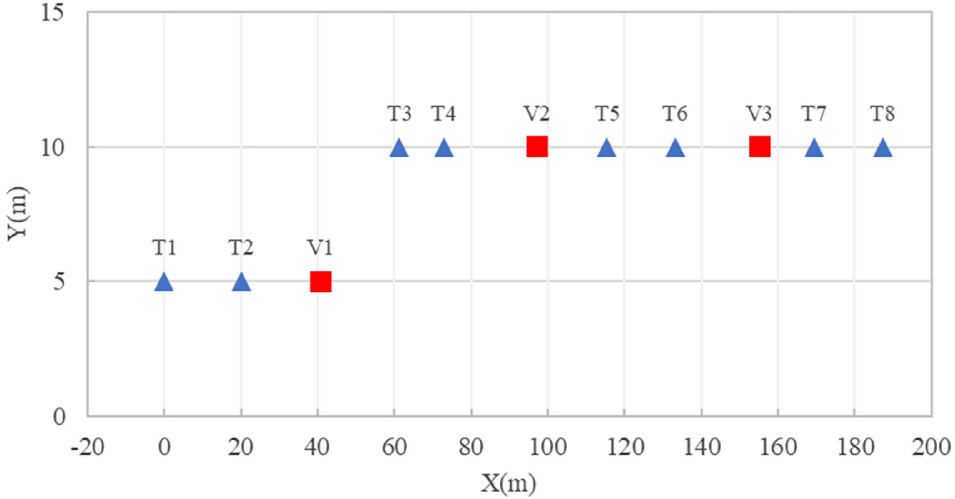
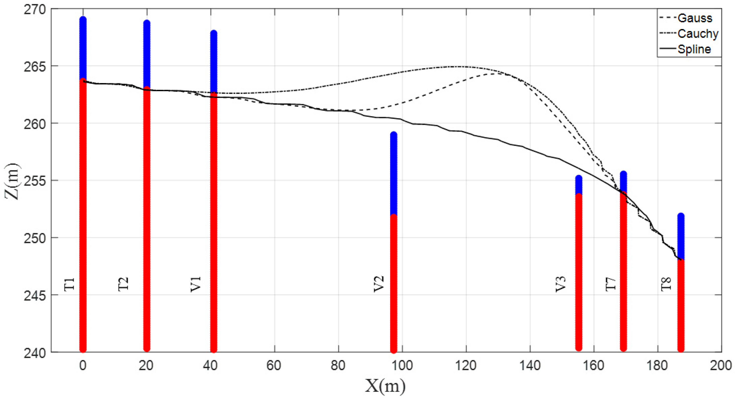
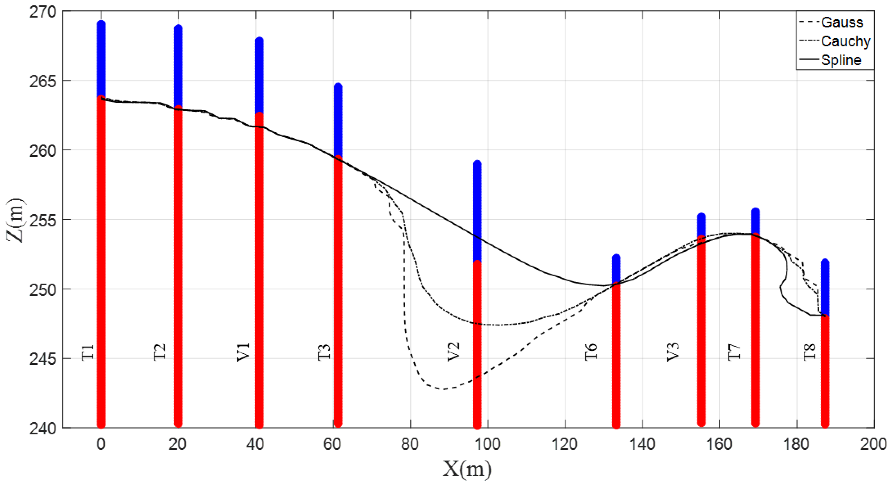
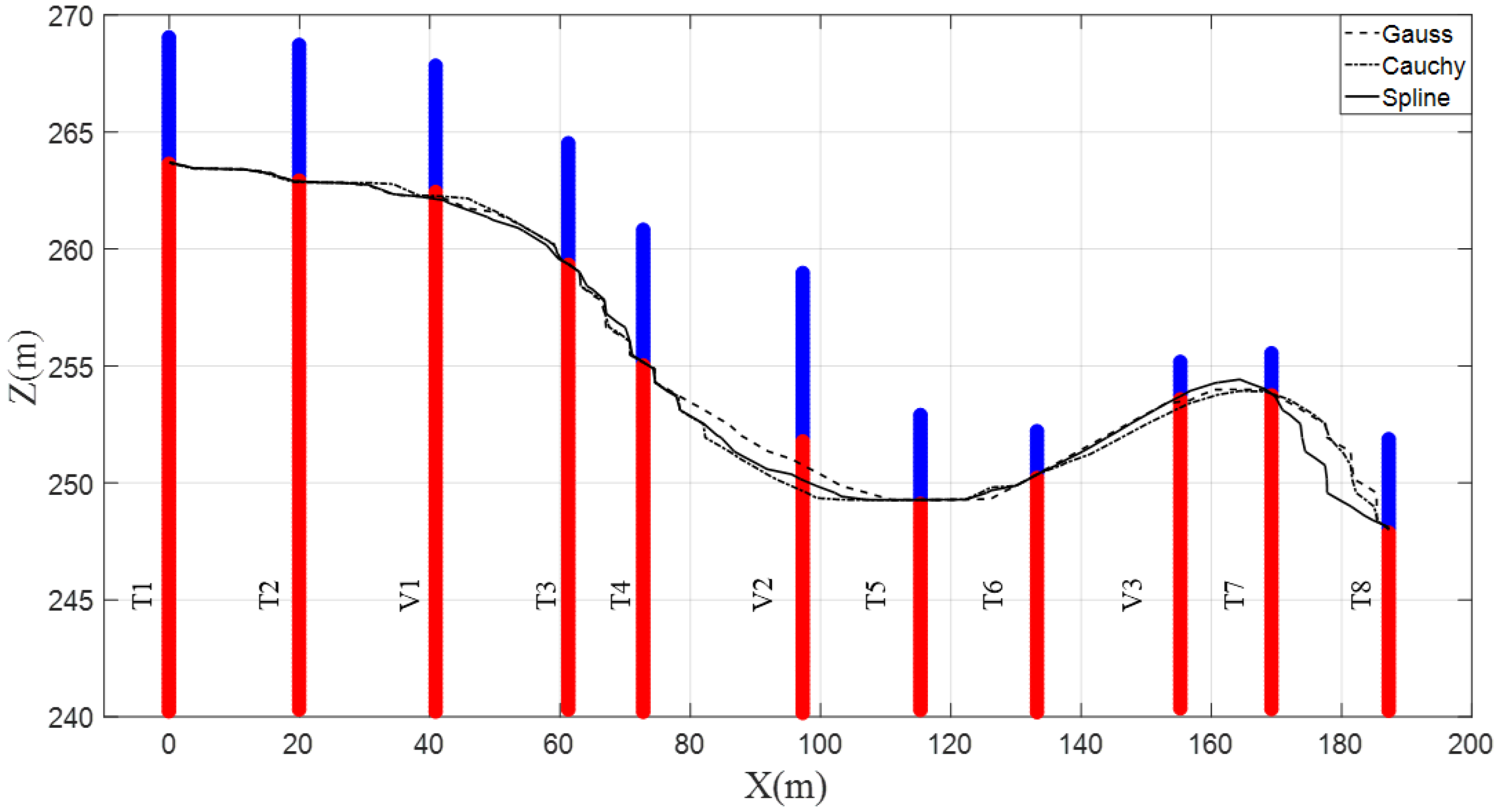
4.1. Two-Dimensional Analysis

In the two-dimensional case, a total of 11 boreholes, as shown in Figure 2, were selected for study, 8 of which were used as training data (labeled by blue triangles in Figure 2) and 3 of which were used as validation data (labeled by red squares in Figure 2). The X-axis and Y-axis represent two directions in the horizontal plane and Z represents the directions of depth. The training and validation dataset contained the information of the spatial location and the type of stratum. The site size was 210 m long × 15 m wide × 30 m deep. The sampling interval along the depth direction was 0.1 m. The 8 training boreholes were used to train a RVM model, tuning the model parameters, while the 3 validation boreholes were used to examine the performance of the proposed model.

In this paper, Gauss, spline, and Cauchy kernel functions were employed for the training of RVM models. In order to directly compare the prediction results obtained from different kernel functions, the stratigraphic interfaces predicted by the proposed RVM method with different kernel functions were plotted in a figure. Three kinds of training data (four training holes, six training holes, and eight training holes) were used for a RVM training in order to check the influence of the number of boreholes on the predictive performance of a constructed RVM model.

Figure 3 shows the results of the stratigraphic stratification predicted by the constructed RVM with four training boreholes. It is seen that the predicted results at the four training boreholes (T1, T2, T7, T8) were consistent with the real situation. The proposed RVM model gave good prediction results on the V1 test borehole. However, in the V2 test borehole and the V3 test borehole, the proposed method showed a bad performance. In the V2 test borehole, the error between the predicted interface depth and the real interface depth reached more than 8.4 m, the results of which are summarized in

Table 1. Prediction results for three kernel functions in the case of four training boreholes.

Kernel Function	$\mathbf{\Omega }$ for Training Data	$\mathbf{\Omega }$ for Validation Data	$\mathbf{\Delta }$ (m) for V2
Spline	1.0	0.8544	8.4
Cauchy	1.0	0.8576	12.4
Gauss	1.0	0.8479	9.4

. Prediction accuracies estimated by Equation (13) for three Kernel functions are also given in Table 1. The “accuracy of testing data” in Table 1 means the average value of the prediction accuracies of all four training and three test boreholes. It is not surprising to see that the prediction accuracies of the three kernel functions at the training boreholes were all equal to 1, which aligns well with the results in Figure 3. The predictive accuracies of the proposed RVM model ranged from 0.84 to 0.86.

Figure 4 shows the results of the stratigraphic stratification predicted by the constructed RVM with six training boreholes. It is worth noting that, compared with using four training boreholes, the prediction accuracy at the V3 test borehole was greatly improved by using six training boreholes. Specifically, at the V3 test borehole, the prediction accuracy reached 95% and the absolute boundary depth error ∆ did not exceed 0.4 m. It is well known that an extrapolation prediction is often more difficult than an interpolation prediction when using machine learning methods. Therefore, the addition of the T6 borehole to training data may be one of the main reasons for the significant improvement of the prediction accuracy at the V3 test borehole. By using 6 training holes, results prediction accuracies and absolute boundary depth errors for three kernel functions are given in

Table 2. Results of the predictive accuracy $\mathsf{\Omega }$ for six training boreholes.

Kernel Function	V1	V2	V3	ALL
Spline	0.9712	0.9053	0.9733	0.9515
Cauchy	0.9712	0.7684	1.0	0.9159
Gauss	0.9640	0.5684	0.9867	0.8544

and

Table 3. Results of the absolute boundary depth error $\Delta$ for six training boreholes.

Kernel Function	V1	V2	V3	ALL
Spline	0.8	1.8	0.4	1.0
Cauchy	0.8	4.4	0.2	1.8
Gauss	1.0	8.0	0.2	3.1

. It is seen that, compared with Table 1, the predictive performances on the testing data were largely improved. The proposed RVM model with the Gauss kernel function gave the lowest predictive accuracy, which was 0.8544, while the built RVM model with the spline kernel function was the best one, with the highest accuracy of 0.9515 and the lowest absolute boundary depth error of 1.0 m.

Figure 5 plots the results of the stratigraphic stratification predicted by the proposed RVM method trained with eight boreholes. Generally, the prediction results at the three test holes were good. It can be found from Figure 5 that the prediction result at the test borehole V2 was the worst among the three test boreholes, although the prediction accuracy of Gauss kernel function was 91% and the prediction accuracies of other two kinds of kernel functions were higher than 85%. The results of prediction accuracy for the case of eight training boreholes are given in

Table 4. Results of the predictive accuracy $\mathsf{\Omega }$ for eight training boreholes.

Kernel Function	V1	V2	V3	ALL	Execution Time [sec]
Spline	0.9856	0.9053	1.0	0.9644	6910
Cauchy	0.9928	0.8842	0.9733	0.9547	7220
Gauss	0.9856	0.9368	0.9867	0.9709	7015

and

Table 5. Results of the absolute boundary depth error $\Delta$ for eight training boreholes.

Kernel Function	V1	V2	V3	ALL
Spline	0.4	1.7	0	0.7
Cauchy	0.2	2.0	0.4	0.9
Gauss	0.4	1.2	0.2	0.6

. By using eight training holes, prediction accuracies for three kernel functions are given in Table 4. When the number of training boreholes was relatively small and the distance between the training borehole and the test borehole was large (for example, the data in Table 2 corresponding to six training holes), prediction results using spline kernel functions were better than those of the other two kernel functions. However, when the number of training holes increased, comparing with the results in Table 2, the prediction accuracy using Gauss kernel functions was greatly increased from 0.8544 to 0.9709 and the mean of the absolute boundary depth error was sharply decreased from 3.1 m to 0.6 m, while the prediction accuracy using spline kernel functions was slightly increased from 0.9515 to 0.9644 and the mean of the absolute boundary depth error declined from 1.0 m to 0.7 m. It can be concluded that the Gauss kernel function is more suitable to deal with nonlinear problems and is more sensitive to the number of training data. Therefore, when there are more geotechnical investigation data, it is more appropriate to choose Gauss kernel function for training a RVM, but when there are few geotechnical investigation data, it is better to use spline kernel functions for RVM model trainings. However, the above conclusion may only apply to the present case study, not suitable to be generalized to other cases.

In addition, the computational time required for RVM trainings on a computer with an Intel Core i7-8700 3.2 GHz CPU are also reported in Table 4. As shown in Table 4, it took 6910 s to finish training a RVM model with a spline kernel function, and 7220 s for a Cauchy kernel function, and 7015 s for a Gauss kernel function. In general, there was no significant difference between them.

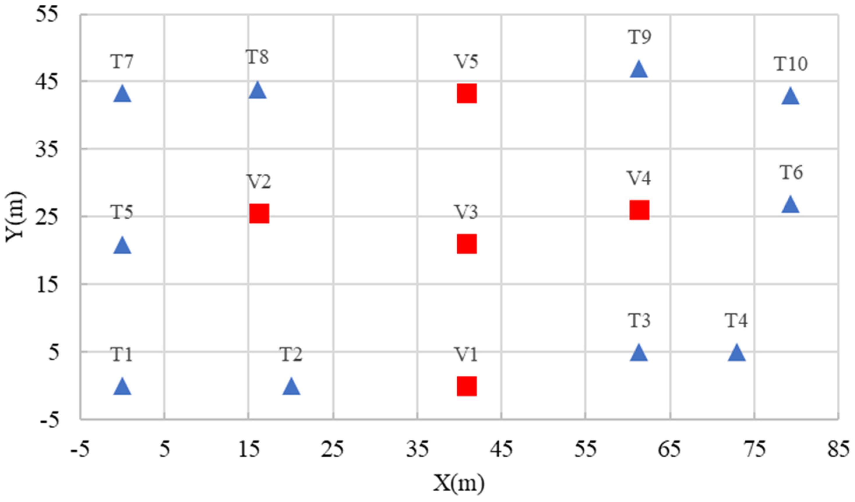
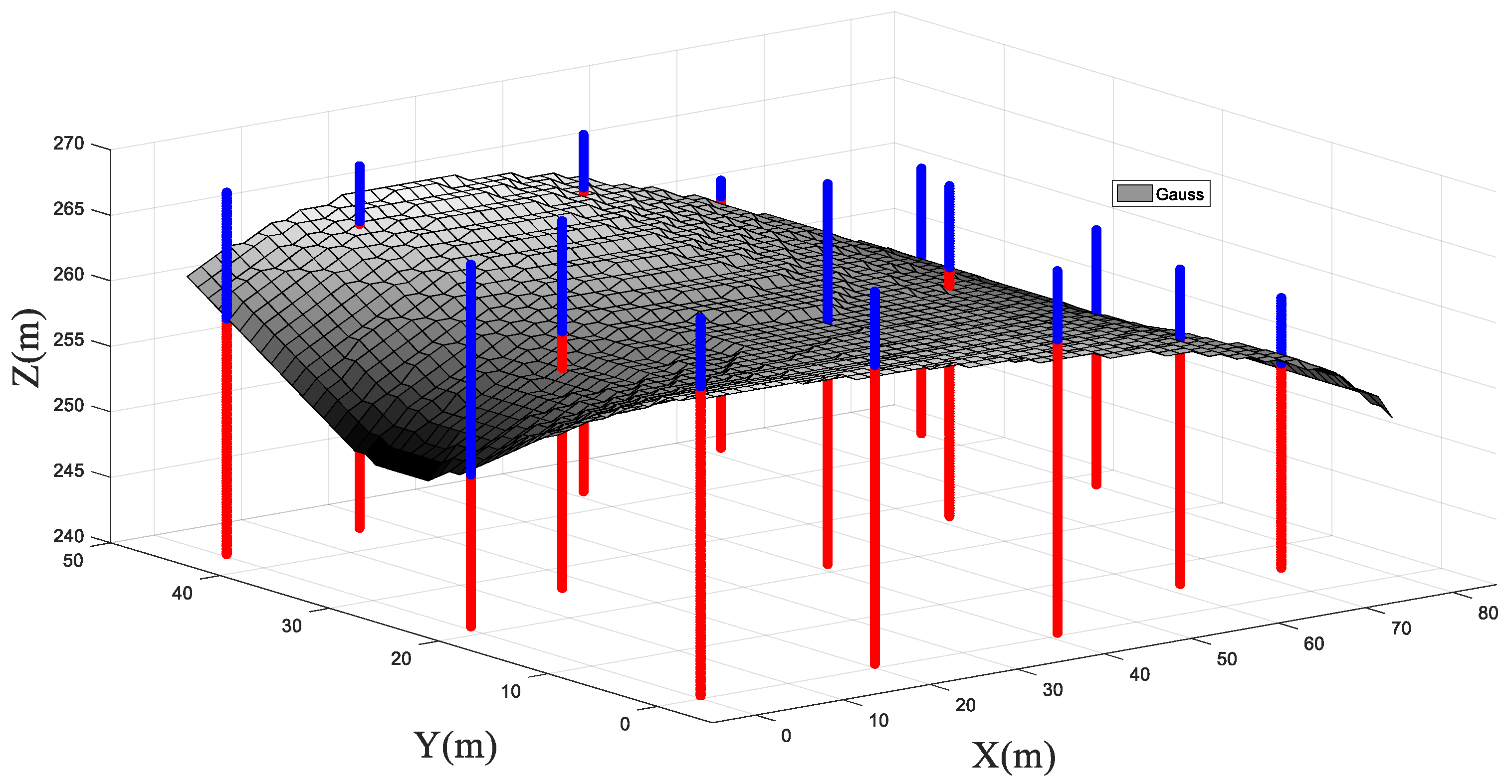
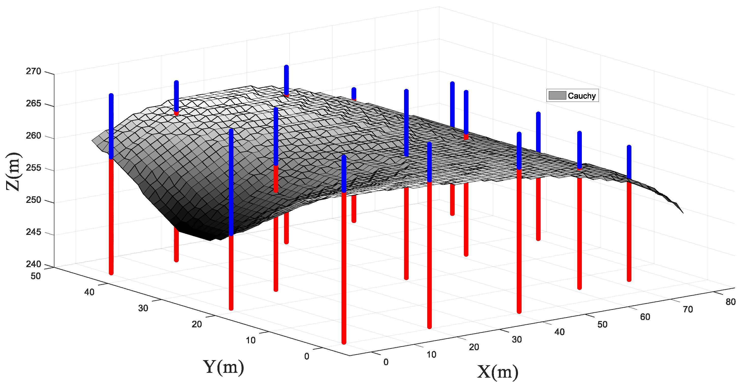
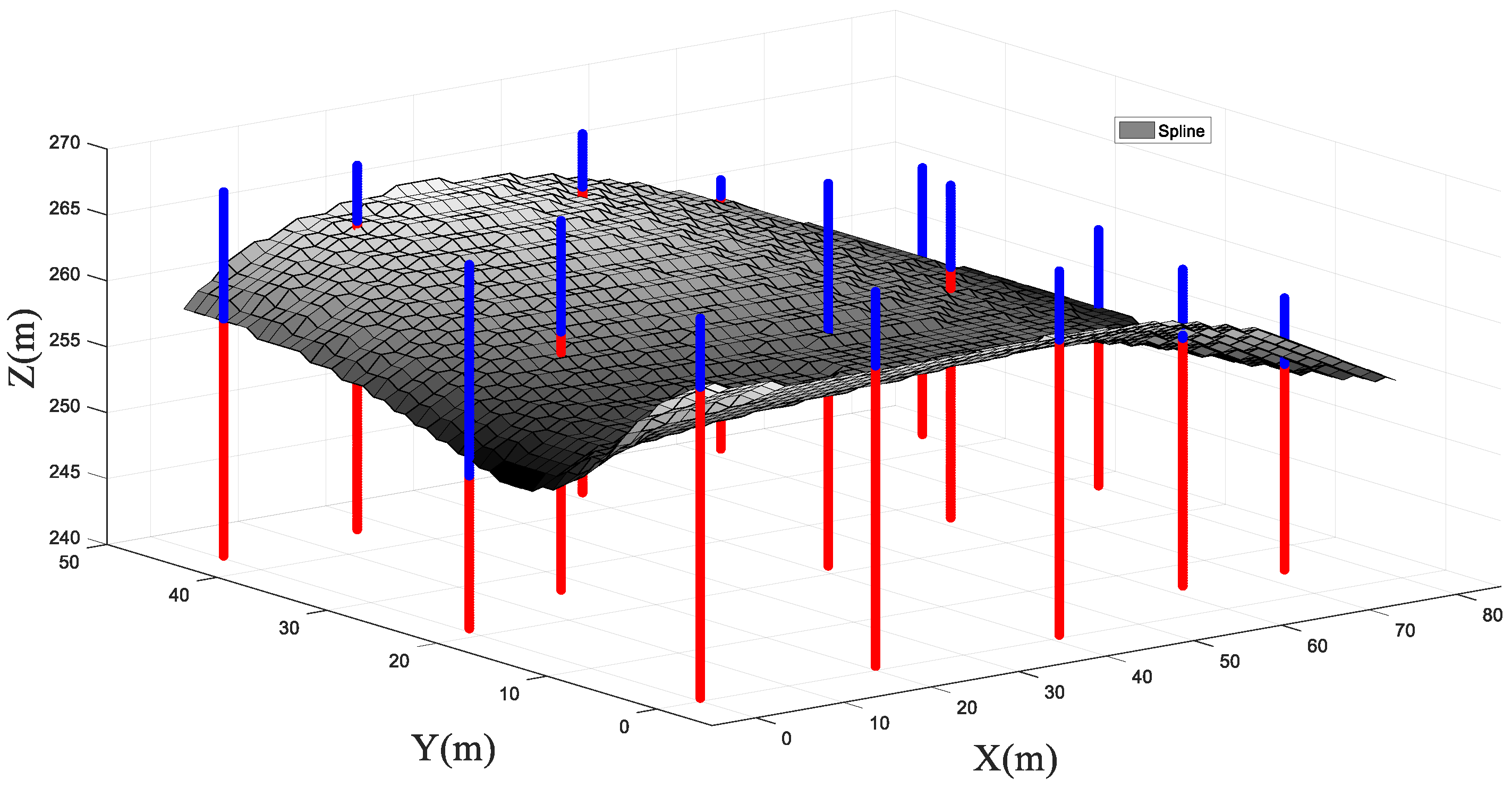
4.2. Three-Dimensional Analysis

This section aims to check the performance of the proposed method on three-dimensional spatial distribution of the subsurface interface between two layers. The layout of 15 boreholes is shown in Figure 6, including 10 for training (T1–T10, labeled by blue triangles) and 5 for testing (V1–V5, labeled by red squares). The training and validation dataset included the spatial location and the type of soil and rock stratum, which were taken from the same project in the 2D analysis case. The site size was 90 m long × 50 m wide × 30 m deep. The sampling interval along the depth direction was 0.1 m. These borehole data were taken from the Dajiang project. In this section, all 10 training boreholes were used to build RVM models to predict the stratigraphic boundary in three-dimensional space and three kernel functions (Gauss, Cauchy, and spline) were considered. The predicted rockhead interfaces from different kernel functions were compared and studied.

Figure 7 plots the results of the rockhead boundary predicted by the proposed RVM method using Gauss kernel function trained with ten boreholes. The results of three kernel functions are summarized in

Table 6. Results of the predictive accuracy $\mathsf{\Omega }$ for 10 training boreholes.

Kernel Function	Spline	Cauchy	Gauss
V1	0.9784	0.9640	0.9712
V2	0.9504	0.8582	0.9078
V3	0.9589	0.8973	0.9110
V4	0.9291	0.9764	0.9606
V5	0.9927	0.9927	1.0000
ALL	0.9623	0.9362	0.9493
Execution Time (sec)	8012	9040	8520

and

Table 7. Results of the absolute boundary depth error $\Delta$ for 10 training boreholes.

Kernel Function	Spline	Cauchy	Gauss
V1(m)	0.4	1.0.	0.8
V2(m)	1.4	4.0	2.6
V3(m)	1.0	3.8	2.4
V4(m)	1.8	0.6	1.0
V5(m)	0.4	0.0	0.0
Mean(m)	1.0	1.8	1.4

. When we used Gauss kernel functions for RVM model trainings, it can be seen from Figure 7 that the prediction results of the V1 and V5 test boreholes were the best, and the mean of the prediction accuracies were 97.12% and 100%, respectively, according to column 3 of Table 6. The mean of prediction accuracy of the V4 test borehole was 96.06%, while the mean of prediction accuracies of the V2 and V3 test boreholes were 90.18% and 91.1%, respectively, while the absolute boundary depth errors for the V2 and V3 test boreholes were respectively 2.6 m and 2.4 m, according to column 3 of Table 7

Figure 8 plots the results of the rockhead boundary predicted by the proposed RVM method using Cauchy kernel functions trained with 10 boreholes. It can be seen from Table 6 that there is little difference between the results predicted by using Cauchy kernel functions and Gauss kernel functions. However, the prediction results of the V2 and V3 test boreholes using Cauchy kernel functions were worse than those using Gauss kernel functions. It can be seen from Table 7 that using Cauchy kernel function, the absolute boundary depth errors of the V2 and V3 test boreholes were, respectively, 4.0 m and 3.8 m. At the V1 and V5 test boreholes, the prediction accuracies of Cauchy kernel functions were respectively 96.40% and 99.27%, according to Table 6.

Similar to the two-dimensional analysis case, the running time required for RVM trainings using three kernel functions are given in Table 6. As shown in Table 6, it took 8012 s for a spline kernel function, 8560 s for a Cauchy kernel function, and 9040 s for a Gauss kernel function. The running times in Table 6 are longer than those in Table 4. This is probably because more training borehole data were involved in this case.

Figure 9 plots the results of the rockhead positions predicted by the proposed RVM method with the spline kernel function trained with 10 boreholes. It can be seen from Table 6 and Table 7 that the weighted average prediction accuracy of the proposed method using a spline kernel function on the five testing boreholes was 96.23%, which is better than that of the other two kernel functions. At the V1 and V5 test boreholes, the prediction accuracies of spline kernel function were respectively 97.84% and 99.27%. At the V2 test borehole, the absolute boundary depth error was 1.4 m.

By analyzing the above prediction results obtained by using the three kernel functions, it can be concluded that the prediction results at the V1 and V5 testing boreholes were generally better than those at V2, V3, and V4 test boreholes. The main reason for this phenomenon is that there were four training boreholes around the V1 and V5 test boreholes, and the distances between the training boreholes and the V1 and V5 test boreholes were small. Comparing the prediction results of the three kernel functions, it can be found that the prediction result of spline kernel function was the best, which was different from the two-dimensional analysis, and the proposed method with a Spline kernel function performed better in the area with a fast change in geological formation.

5. Conclusions and Discussions

This paper studies the prediction of geological boundary using borehole data. For this issue, the machine learning method of relevant vector machine was employed. The relevant vector machine is equipped with many advantages such as good learning and generalization ability, flexible choice of kernel function, and sparse relevant vectors. The basics of the relevant vector machine are introduced in this paper, and the optimal width parameter of kernel functions, which is an important parameter required for model training and prediction, was determined by optimizing the marginal likelihood using the particle swarm optimization (PSO) algorithm. Three types of kernel function (spline, Cauchy, and Gauss kernel function) were employed in this work. The prediction results obtained from different kernel functions were evaluated by calculating the prediction accuracy and the absolute boundary depth error.

In the 2D case analysis, 11 boreholes (8 training holes and 3 test holes) were studied. This may result from the fact that an interpolation prediction is often easier and more precise than an extrapolation prediction when using machine learning methods. For this case, as for the selection of kernel function, the comparison of different kernel functions showed that with the increase of training samples (6 training holes and 8 training holes), the prediction accuracy of Gaussian kernel function was better than that of other kernel functions. That is, when there are enough geotechnical investigation data, it is more appropriate to choose a Gaussian kernel function to train a RVM model. However, when there are few geotechnical investigation data, it is best to use spline kernel function for RVM training. However, it has to be noted that the above conclusion only applies to the present case study, and more tests are needed for this to be generalized in a future study.

In the 3D case analysis, 15 boreholes were investigated. The results showed that the prediction result of the RVM model with a spline kernel function was the best, and performed better in the area with a fast change in geological formation.

In this paper, the machine learning method of relevant vector machine (RVM) was firstly used to predict the stratigraphic profile based on the limited geotechnical borehole data. The hyper-parameters of the kernel function were determined by maximizing the marginal likelihood using the particle swarm optimization algorithm. The proposed method had benefit to give a sparse predictive mode that was able to avoid both underfitting and overfitting issues. In order to give a deep study of the proposed model performance, three kernel functions were employed to study the prediction performance in a two-dimensional case study and a three-dimensional case study. This research is able to fill the gap of applying the method of a RVM to predict the stratigraphic formation in the geotechnical community. It can be concluded that the proposed method has the potential of addressing the problem of three-dimensional geotechnical stratum reconstruction using geotechnical investigation data, provide convenience for the design and construction of geotechnical engineering, and pave a way for the data-centric geotechnical site characterization.

There are still some problems worthy of further study. In the 2D case study, as for the selection of kernel function, the comparison of different kernel functions showed that with the increase of training samples (6 training holes and 8 training holes), the prediction accuracy of Gaussian kernel function was better than that of other kernel functions. That is, when there are enough geotechnical investigation data, it is more appropriate to choose a Gaussian kernel function to train a RVM model. However, when there are few geotechnical investigation data, it is best to use spline kernel function for the RVM training. However, it has to be noted that the above conclusion only applies to the present case study, and more tests are needed for this to be generalized in a future study. Moreover, the presented study shows that the model with a spline kernel function has a better generalization ability in the case of 3D analysis. This is possibly due to the fact that in the three-dimensional stratum stratification prediction problem, the influence of the cross-boreholes influence needs to be considered, and a spline kernel function differs in the mathematical expressions from a Gaussian kernel one and shows a slow convergence velocity in the range of the estimated width parameter. Therefore, the reason that for proposed method on two-dimensional and three-dimensional problems showing different performance with difference kernel functions will be studied and clarified in the future.

There is a possible uncertainty for the proposed method. Even though the width parameter of a kernel function is determined by the particle swarm optimization algorithm, it is subjected to an uncertainty of global solution issue. This is a possible risk that the PSO fails to give a global best value of the width parameter, not obtaining the highest marginal likelihood. This may be improved if a more advanced optimization method can be used, for example to combine a global optimization algorithm and a local optimization algorithm.

References

1. Deng, Z.P.; Jiang, S.H.; Niu, J.T.; Pan, M.; Liu, L.L. Stratigraphic uncertainty characterization using generalized coupled Markov chain. Bull. Eng. Geol. Environ. 2020, 79, 5061–5078. [Google Scholar] [CrossRef]
2. Phoon, K.K.; Ching, J.; Shuku, T. Challenges in data-driven site characterization. Georisk Assess. Manag. Risk Eng. Syst. Geohazards 2022, 16, 114–126. [Google Scholar] [CrossRef]
3. Zhang, W.; Gu, X.; Tang, L.; Yin, Y.; Liu, D.; Zhang, Y. Application of machine learning, deep learning and optimization algorithms in geoengineering and geoscience: Comprehensive review and future challenge. Gondwana Res. 2022, 109, 1–17. [Google Scholar] [CrossRef]
4. Liu, L.L.; Cheng, Y.M.; Pan, Q.J.; Dias, D. Incorporating stratigraphic boundary uncertainty into reliability analysis of slopes in spatially variable soils using one-dimensional conditional Markov chain model. Comput. Geotech. 2020, 118, 103321. [Google Scholar] [CrossRef]
5. Liu, L.L.; Wang, Y. Quantification of stratigraphic boundary uncertainty from limited boreholes and its effect on slope stability analysis. Eng. Geol. 2022, 306, 106770. [Google Scholar] [CrossRef]
6. Gong, W.; Tang, H.; Wang, H.; Wang, X.; Juang, C.H. Probabilistic analysis and design of stabilizing piles in slope considering stratigraphic uncertainty. Eng. Geol. 2019, 259, 105162. [Google Scholar] [CrossRef]
7. Qi, X.; Wang, H.; Chu, J.; Chiam, K. Two-dimensional prediction of the interface of geological formations: A comparative study. Tunn. Undergr. Space Technol. 2022, 121, 104329. [Google Scholar] [CrossRef]
8. Qi, X.; Wang, H.; Pan, X.; Chu, J.; Chiam, K. Prediction of interfaces of geological formations using the multivariate adaptive regression spline method. Undergr. Space 2021, 6, 252–266. [Google Scholar] [CrossRef]
9. Li, Z.; Wang, X.; Wang, H.; Liang, R.Y. Quantifying stratigraphic uncertainties by stochastic simulation techniques based on Markov random field. Eng. Geol. 2016, 201, 106–122. [Google Scholar] [CrossRef]
10. Li, X.Y.; Zhang, L.M.; Li, J.H. Using conditioned random field to characterize the variability of geologic profiles. J. Geotech. Geoenviron. Eng. 2016, 142, 04015096. [Google Scholar] [CrossRef]
11. Han, L.; Wang, L.; Zhang, W.; Geng, B.; Li, S. Rockhead profile simulation using an improved generation method of conditional random field. J. Rock Mech. Geotech. Eng. 2022, 14, 896–908. [Google Scholar] [CrossRef]
12. Zhang, J.Z.; Liu, Z.Q.; Zhang, D.M.; Huang, H.W.; Phoon, K.K.; Xue, Y.D. Improved coupled Markov chain method for simulating geological uncertainty. Eng. Geol. 2022, 298, 106539. [Google Scholar] [CrossRef]
13. Shi, C.; Wang, Y. Data-driven construction of Three-dimensional subsurface geological models from limited Site-specific boreholes and prior geological knowledge for underground digital twin. Tunn. Undergr. Space Technol. 2022, 126, 104493. [Google Scholar] [CrossRef]
14. Song, S.; Mukerji, T.; Hou, J. Geological facies modeling based on progressive growing of generative adversarial networks (GANs). Comput. Geosci. 2021, 25, 1251–1273. [Google Scholar] [CrossRef]
15. Feng, R.; Grana, D.; Mukerji, T.; Mosegaard, K. Application of Bayesian Generative Adversarial Networks to Geological Facies Modeling. Math. Geosci. 2022, 54, 831–855. [Google Scholar] [CrossRef]
16. Liu, Q.; Liu, W.; Yao, J.; Liu, Y.; Pan, M. An improved method of reservoir facies modeling based on generative adversarial networks. Energies 2021, 14, 3873. [Google Scholar] [CrossRef]
17. Tipping, M.E. Sparse Bayesian learning and the relevance vector machine. J. Mach Learn. Res. 2001, 1, 211–244. [Google Scholar]
18. Tipping, M. The relevance vector machine. Adv. Neural Inf. Process. Syst. 1999, 12, 652–658. [Google Scholar]
19. Bishop, C.M.; Nasrabadi, N.M. Pattern Recognition and Machine Learning; Springer: New York, NY, USA, 2006; Volume 4, p. 738. [Google Scholar]
20. Li, Y.; Chen, J.; Shang, Y. An RVM-based model for assessing the failure probability of slopes along the Jinsha River, close to the Wudongde dam site, China. Sustainability 2016, 9, 32. [Google Scholar] [CrossRef]
21. Zhao, H.; Yin, S.; Ru, Z. Relevance vector machine applied to slope stability analysis. Int. J. Numer. Anal. Methods Geomech. 2012, 36, 643–652. [Google Scholar] [CrossRef]
22. Pan, Q.J.; Leung, Y.F.; Hsu, S.C. Stochastic seismic slope stability assessment using polynomial chaos expansions combined with relevance vector machine. Geosci. Front. 2021, 12, 405–414. [Google Scholar] [CrossRef]
23. Samui, P. Application of relevance vector machine for prediction of ultimate capacity of driven piles in cohesionless soils. Geotech. Geol. Eng. 2012, 30, 1261–1270. [Google Scholar] [CrossRef]
24. Samui, P. Least square support vector machine and relevance vector machine for evaluating seismic liquefaction potential using SPT. Nat. Hazards 2011, 59, 811–822. [Google Scholar] [CrossRef]
25. Abd-Elwahed, M.S. Drilling Process of GFRP Composites: Modeling and Optimization Using Hybrid ANN. Sustainability 2022, 14, 6599. [Google Scholar] [CrossRef]
26. Esmaeili-Falak, M.; Katebi, H.; Vadiati, M.; Adamowski, J. Predicting triaxial compressive strength and Young’s modulus of frozen sand using artificial intelligence methods. J. Cold Reg. Eng. 2019, 33, 04019007. [Google Scholar] [CrossRef]
27. Yuan, J.; Zhao, M.; Esmaeili-Falak, M. A comparative study on predicting the rapid chloride permeability of self-compacting concrete using meta-heuristic algorithm and artificial intelligence techniques. Struct. Concr. 2022, 23, 753–774. [Google Scholar] [CrossRef]
28. Ge, D.M.; Zhao, L.C.; Esmaeili-Falak, M. Estimation of rapid chloride permeability of SCC using hyperparameters optimized random forest models. J. Sustain. Cem.-Based Mater. 2022, 5, 1–19. [Google Scholar] [CrossRef]
29. Gong, Y.-L.; Hu, M.-J.; Yang, H.-F.; Han, B. Research on application of ReliefF and improved RVM in water quality grade evaluation. Water Sci. Technol. 2022, 83, 799–810. [Google Scholar] [CrossRef] [PubMed]
30. Li, T.; Zhou, M.; Guo, C.; Luo, M.; Wu, J.; Pan, F.; Tao, Q.; He, T. Forecasting crude oil price using EEMD and RVM with adaptive PSO-based kernels. Energies 2016, 9, 1014. [Google Scholar] [CrossRef]
31. Tao, H.; Al-Bedyry, N.K.; Khedher, K.M.; Luo, M. River water level prediction in coastal catchment using hybridized relevance vector machine model with improved grasshopper optimization. J. Hydrol. 2021, 598, 126477. [Google Scholar] [CrossRef]
32. Poli, R.; Kennedy, J.; Blackwell, T. Particle swarm optimization. Swarm Intell. 2007, 1, 33–57. [Google Scholar] [CrossRef]
33. Germin Nisha, M.; Pillai, G.N. Nonlinear model predictive control with relevance vector regression and particle swarm optimization. J. Control. Theory Appl. 2013, 11, 563–569. [Google Scholar] [CrossRef]
34. Sengupta, S.; Basak, S.; Peters, R.A. Particle Swarm Optimization: A survey of historical and recent developments with hybridization perspectives. Mach. Learn. Knowl. Extr. 2018, 1, 10. [Google Scholar] [CrossRef]
Figure 1. Flow chart of the proposed method.
Sustainability 14 10122 g001
Figure 2. Layout of 11 boreholes in two-dimensional analysis.
Sustainability 14 10122 g002
Figure 3. Stratigraphic stratification predictions for a two-dimensional section (four training boreholes).
Sustainability 14 10122 g003
Figure 4. Stratigraphic stratification prediction of two-dimensional section (six training holes).
Sustainability 14 10122 g004
Figure 5. Stratigraphic stratification prediction of two-dimensional section (eight training holes).
Sustainability 14 10122 g005
Figure 6. Layout of 15 boreholes for dimensional analysis.
Sustainability 14 10122 g006
Figure 7. A 3D diagram of stratigraphic stratification (Gauss kernel function).
Sustainability 14 10122 g007
Figure 8. A 3D diagram of stratigraphic stratification (Cauchy kernel function).
Sustainability 14 10122 g008
Figure 9. A 3D diagram of stratigraphic stratification (spline kernel function).
Sustainability 14 10122 g009