Study on the Influencing Factors of CO₂ from the Perspective of CO₂ Mitigation Potentials

Abstract

As the world pays more attention to carbon reduction, it is of great significance to identify the factors of CO₂ to achieve carbon peaking and carbon neutrality goals for China. Therefore, this paper explores the factors of CO₂ from the perspective of CO₂ mitigation potentials (CESP) and analyzes the heterogeneity of each factor. We first employ the DEA-IDA model framework to analyze the CESP and influencing factors of each region, and then use geographically and temporally weighted regress to analyze the spatiotemporal heterogeneity of influencing factors, the efficiency, coal proportion, energy intensity, per capita GDP, urbanization rate, electrification rate, trade, economic structure, and climate conditions. The research results show that: (1) for 1 unit increase in per capita CO₂, the per capita CESP increases by 0.56 units. The CESP of the central and western regions is greater than that of the eastern regions, and the improvement of resource utilization efficiency can achieve the peak in advance. (2) Per capita GDP and energy intensity are the main positive factor and negative factor, respectively, and the impact of efficiency changes on CESP is mostly positive. (3) Efficiency is the most influential factor affecting the CESP; among them, a 1% increase in efficiency in Hebei can reduce the CESP of 62.47 Mt. In regions dominated by clean power, the impact of electrification rates is negative. The rest of the factors also showed spatiotemporal heterogeneity. Our findings have important policy implications, especially in how to effectively reduce carbon emissions to formulate more appropriate policy.

1. Introduction

Currently, sustainable development has gradually become a global issue, which requires that the advancement of the society should not be at the expense of the environment [1]. Since the late 1980s, mitigating global warming has become an important issue for mankind [2]. Extreme weather events, failure of measures to control climate change, major natural disasters, biodiversity loss, and ecosystem degradation are most likely to have severe impacts. In recent years, rapid economic growth has paid serious resource and environmental costs [3]. Then, climate change affects economic growth by affecting productivity and labor force. Therefore, reducing CO₂ and air pollutants is the primary goal of energy and environmental policy in the world.

After the reform of the economy, China has developed rapidly; meanwhile, it has brought serious environmental problems. According to the statistics of CO₂, China became the world’s largest carbon emitter in 2007 [4], accounting for 21% of global CO₂ [5]. Then, China has actively undertaken the responsibility of emission reduction and pledged to strive to achieve carbon peak by 2030 and carbon neutrality by 2060. To achieve the “dual carbon” goal, the related planning calls for accelerating green and low-carbon development and reducing carbon intensity. Therefore, facing the great pressure of environmental protection, China should identify the key factors and obstacles and formulate targeted policy recommendations.

Decomposition analysis has been widely applied by scholars in the analysis factors of energy, CO₂, pollutants, etc. Index decomposition analysis (IDA), structural decomposition analysis (SDA), and production-theoretical decomposition analysis (PDA) are the three main categories in decomposition analysis. In 1991, IDA was employed in energy analysis and environmental analysis [6]. Torvanger [7] employed IDA to decompose carbon emissions into six impact primers. After that, IDA has been widely employed in the study of influencing factors at the national level and industry level [8,9,10,11,12]. The SDA method, from the economic system, explores the factors affecting carbon emissions based on the input–output table [13,14,15], but it has strict requirements on data and needs to be analyzed by input–output tables. PDA method explores influencing factors through combination decomposition method and data envelopment analysis (DEA) method [16,17,18]. PDA, proposed by Zhou and Ang [19], is applied to study more potential influencing factors of CO₂ in OECD. Compared with the latter two methods, IDA has many advantages. First, from the energy system, IDA is easily able to study drivers at the macro level, which can help policy makers formulate targeted policies [20]. Second, it can easily analyze and compare the differences of carbon emissions in different regions without high requirements for data [21,22].

Low efficiency and resource misallocation will lead to excessive carbon emissions, while the carbon reduction potential (CESP) is the carbon emission generated for such reasons. CESP can be reduced by improving resource utilization efficiency and optimizing resource allocation. DEA is applied in many aspects, including energy and environmental evaluation [23,24,25,26]. Total factor energy efficiency (TFEE), calculated by DEA, is used to study energy efficiency in the study [27]. They concluded some areas of inefficiency in China. Scholars also employ DEA to investigate energy saving and CO₂ reduction potential [28,29,30,31,32,33]. The above IDA approach can investigate single-factor efficiency. While it quantifies the impact of “absolute” efficiency using factors such as energy intensity, it cannot assess “relative” efficiency. DEA can evaluate “relative” efficiency to complement this shortcoming. The advantage of it is that we could investigate the potential in energy and carbon emissions by improving efficiency; however, the effect of absolute efficiency could not be identified sufficiently. Then, the ZA method, proposed by Zhou and Ang [19], combines DEA and decomposition analysis. The method is an extension of DEA, but efficiency in the form of ratio does not perfectly reflect changes in relative efficiency over time. Thus, PDA could not investigate the efficiency change. Takayabu et al. [30] combined the IDA and DEA models to overcome some of the above defects, and studied the impact of three different efficiencies. This paper also employs it to study the factors of CO₂ and CESP.

Here, we first investigate the differences between CESP and carbon emissions in each region. Then a DEA–IDA analysis framework was used to explore the factors of CO₂ and CESP. Finally, the heterogeneity, in time and space, of factors of CESP and CO₂ is studied by a spatial econometric model, geographically and temporally weighted regress (GTWR). The contributions of this paper are as follows: (1) we analyze the importance of CESP in the realization of dual carbon goals, and compare the differences between CESP and CO₂. (2) The DEA–IDA framework was used to explore five factors affecting carbon emissions and CESP. (3) In this paper, GTWR was employed to investigate the spatio-temporal heterogeneity of factors of CESP and CO₂ in 30 provinces, providing a reference for the formation of specific policy implications.

This study is organized as follows. Section 2 provides methodology. We describe data in Section 3. Section 4 presents and discusses the results. Finally, we conclude this study.

2. Methodology and Data

2.1. Methodology

2.1.1. Data Envelopment Analysis

DEA, a nonparametric method, deals with multi-input and multi-output situations, which has obvious advantages. It avoids the assumption of functional form and is easy to be changed and extended to other forms [19,34,35,36,37,38]. According to Cooper et al. [39], the DEA model can be expressed as the following:

$$\begin{array}{l}\min {\theta }_k\\ {\displaystyle \sum _{i=1}^g{\phi }_i{x}_{ih}\le {\theta }_k}{x}_{kh},h=1,2,\dots ,n\\ {\displaystyle \sum _{i=1}^g{\phi }_i{y}_{il}\ge }{y}_{kl},l=1,2,\dots ,r\\ {\phi }_i\ge 0,i=1,2,\dots ,g\end{array}$$

(1)

The efficiency of the decision-making unit (DMU_K) can be represented by ${\theta }_k$; $1-{\theta }_k$ represents the value that the DMU_K can reduce under the premise of maintaining the existing output, that is, the reduction potential of the input; x is the input index, representing labor, capital, and energy, respectively; y is the output, representing economic output; v represents the weight of DMU_K.

In Equation (1), this can be expressed as:

$${\displaystyle \sum _{i=1}^g{v}_i{x}_{ih}\le {\theta }_k}{x}_{kh}\Rightarrow \begin{array}{l}{\displaystyle \sum _{i=1}^g{v}_i{x}_{{}_{id}}^E\le {\theta }_k}{x}_{{}_{kd}}^E,d=1\\ {\displaystyle \sum _{i=1}^g{v}_i{x}_{is}^{NE}\le {\theta }_k}{x}_{{}_{ks}}^{NE},s=1,2\end{array}$$

(2)

where $x_{{}_{kj}}^E$ represents energy input and $x_{{}_{kj}}^{NE}$ represents non-energy input, namely labor and capital. $1-{\theta }_k$ represents energy-saving potential. The complementarity of energy and other input elements is considered, that is, a simultaneous increase and decrease. Since both capital and labor need the supply of energy, the decrease of energy will cause the decrease of capital and labor, and the decrease of capital and labor will also cause the corresponding energy reduction. Therefore, energy is not considered separately, as in Takayabu [30]. The relevant variables are shown in

Table 1. Definition of input and output variables.

Types of Variables	Variables	Definition
Input variables	energy	total energy consumption
	labor	working population at the end of the year
	capital	capital stock
Output variables	economic output	GDP

.

When calculating the CO₂ reduction potential (CESP), energy sources include coal, coke, petroleum, crude oil, gasoline, kerosene, diesel, fuel oil, LPG, natural gas, and electricity.

2.1.2. Energy Saving and Emission Reduction Potential

The energy saving and emission reduction potential can be understood as the amount that can be reduced after resource optimization, which represents the difference between the optimal production and the actual production. The energy saving potential (EESP) of each region can be obtained, and the CO₂ reduction potential (CESP) can be calculated according to the following formula.

$$EES{P}_k={\displaystyle \sum _{h=1}^{11}\left[(1-{\theta }_k)\times x_{{}_{kh}}^E\right]}$$

(3)

$$\begin{array}{l}CES{P}_k={\displaystyle \sum _{h=1}^{11}\left[(1-{\theta }_k)\times x_{{}_{kh}}^E\times F_{kh}\right]}\\ F_{kh}={\displaystyle \sum _h^{11}{\alpha }_{kh}\times {\beta }_{kh}\times \frac{44}{12}}\end{array}$$

(4)

In the above formula, $x_{{}_{kh}}^E$ represents the consumption of the h-th energy of DMU_K; $F_{kh}$ is the carbon emission factor of the h-th energy; H represents the type of energy; ${\alpha }_{{}_j}^{}$ refers to the standard coal coefficient converted to the j-th energy; β_j represents the carbon emission coefficient of the j-th energy; and 44/12 is the mass conversion coefficient of CO₂ molecules oxidized by carbon atoms. The relevant parameter refers the IPCC [40].

When DMU_K is effective, equal to 1, both EESP and CESP are equal to zero, implying that DMU_K is on the frontier of production and has no potential. EESP is the gap between the observations and the frontier, and greater EESP means greater energy loss. The same is true for CESP. Therefore, DMU_K does not expect a large CESP.

2.1.3. Decomposition Model

According to the Kaya identity [41], we combine the DEA model and IDA model to divide the real carbon emissions into two parts, namely basic carbon emissions (AC) and CESP, and decompose them into five factors.

$$C^t=CES{P}^t+A{C}^t$$

(5)

$$A{C}^t={\displaystyle \sum _{i=1}^{30}\frac{C_{{}_i}^t}{E_{{}_i}^t}\times \frac{E_{{}_i}^t}{GD{P}_{{}_i}^t}\times \frac{GD{P}_{{}_i}^t}{P_{{}_i}^t}}$$

(6)

$$CES{P}^t={\displaystyle \sum _{i=1}^{30}(1-\theta )\times }\frac{C_{{}_i}^t}{E_{{}_i}^t}\times \frac{E_{{}_i}^t}{GD{P}_{{}_i}^t}\times \frac{GD{P}_{{}_i}^t}{P_{{}_i}^t}\times P_{{}_i}^t$$

(7)

Among them, AC represents the optimized carbon emissions, that is, the actual CO₂ minus CESP; C_i represents CO₂ in the i region; E_i is the energy; GDP_i is the economic output; P_i is the population; ${\theta }_i$ is the production efficiency; and 1 − ${\theta }_i$ is the saving potential. This paper mainly studies the energy-related carbon emissions; therefore, ${\theta }_i$ and 1 − ${\theta }_i$ represent the utilization efficiency and the potential saving ratio in energy, respectively.

$$\mathsf{\Delta }{C}_i=C_{{}^i}^t-C_{{}^i}^0=\mathsf{\Delta }ER{P}_i+\mathsf{\Delta }C{E}_i+\mathsf{\Delta }E{I}_i+\mathsf{\Delta }G{P}_i+\mathsf{\Delta }{P}_i$$

(8)

Among them, $\mathsf{\Delta }ER{P}_i$ is the change of CO₂ caused by change of 1 − ${\theta }_i$; $\mathsf{\Delta }C{E}_i$ represents the change of CO₂ caused by the change of emission coefficient ($\frac{C_{{}_i}^{}}{E_{{}_i}^{}}$); $\mathsf{\Delta }E{I}_i$ is the change of CO₂ caused by the change of energy intensity ($\frac{E_{{}_i}^{}}{GD{P}_{{}_i}^{}}$); $\mathsf{\Delta }G{P}_i$ is the change of CO₂ caused by the change of per capita GDP ($\frac{GD{P}_{{}_i}^{}}{P_{{}_i}^{}}$); $\mathsf{\Delta }{P}_i$ is changes in CO₂ caused by changes in population ($P_{{}_i}^{}$).

This paper employs LMDI to solve the contribution of each factor because LMDI can perfectly solve the problem of decomposing residual and zero values. A detailed derivation process can refer to Ang and Wang [42]. Each effect can be calculated according to the following model.

$$\mathsf{\Delta }C(X_j)=\omega (t*)\ln \frac{X_j^t}{X_j^0}$$

(9)

Among them, X_j represents different influencing factors.

$$\omega (t*)=\{\begin{array}{c}\frac{C_i^t-C_i^0}{\ln C_i^t-\ln C_i^0}\\ \\ C_i^0\end{array}\begin{array}{c},C_i^t\ne C_i^0\\ \\ ,C_i^t=C_i^0\end{array}$$

(10)

The contribution of each factor can refer to Appendix B.

2.1.4. Geographically and Temporally Weighted Regress

GTWR considers two attributes, temporal and spatial. Therefore, when studying the heterogeneity of factors, GTWR is closer to reality. The logarithm of CO₂ and CESP is employed as the dependent variable. The specific form of its model is as follows.

$$y_i={\beta }_0({\mu }_i,{\nu }_i,t_i)+{\displaystyle \sum _{k=1}^p{\beta }_k({\mu }_i,{\nu }_i,t_i)x_{ik}+{\epsilon }_i} i=1,2,\dots ,n$$

(11)

$({\mu }_i,{\nu }_i,t_i)$ is the spatiotemporal coordinates (geographic location, and time); ${\beta }_k({\mu }_i,{\nu }_i,t_i)$ is the parameter. Meanwhile, ${\epsilon }_i~N(0,{\sigma }^2)$ and $Cov({\epsilon }_i,{\epsilon }_j)=0$.

Spatiotemporal distance ($d_{ij}^{ST}$) is as follows, referring to the research of Huang et al. [43].

$$d_{ij}^{ST}=\sqrt{\alpha \left[{({\mu }_i-{\mu }_j)}^2+{({\nu }_i-{\nu }_j)}^2\right]+\beta {(t_i-t_j)}^2}$$

(12)

${\omega }_{ij}^{ST}$ is as follows.

$${\omega }_{ij}^{ST}=\exp \left\{-(\frac{\alpha \left[{({\mu }_i-{\mu }_j)}^2+{({\nu }_i-{\nu }_j)}^2\right]+\beta {(t_i-t_j)}^2}{b_{ST}^2})\right\}$$

(13)

${\omega }_{ij}^{ST}$ is spatiotemporal weight function. $b^{ST}$ is the bandwidth determined by AIC.

This paper employs IDA decomposition and the IPAT equation [44] to determine the factors of CO₂, where I is environmental pressure, carbon emissions; P is population size; A is wealth, per capita GDP; and T is technology, energy intensity, and efficiency. The paper also explores the impact of electrification rates and import and export trade on carbon emissions and CESP.

$$\ln C=f(\ln \theta ,\ln EM,\ln EI,\ln GDPP,\ln P,\ln ER,\ln IE,\ln ES,\ln TP,\ln RL)$$

(14)

$$\ln CESP=f(\ln \theta ,\ln EM,\ln EI,\ln GDPP,\ln P,\ln ER,\ln IE,\ln ES,\ln TP,\ln RL)$$

(15)

C represents total carbon emissions; CESP represents carbon emission reduction potential; $\theta$ represents production efficiency; EM represents energy structure (coal consumption/total energy consumption); EI is energy intensity (energy consumption/GDP); GDPP represents per capita GDP; P represents population, since considering the impact of urbanization on CO₂, it represents the urban population; ER represents the electrification rate, the proportion of electricity consumption; and IE represents trade, expressed by total import and export. ES represents economic structure, expressed by the ratio of the added value of the secondary industry to GDP. TP represents the average temperature. RL represents the average precipitation.

2.2. Data

All of the data are from the “China Statistical Yearbook” and “China Energy Statistical Yearbook”, where the provincial GDP and fixed asset investment are converted at constant prices in 2000. The provincial capital stock calculation method is the perpetual inventory method [45]. The specific data descriptions are shown in

Table A1. Sample data of DEA.

	Observations	Min	25%	50%	75%	Max	Mean	Variance
Energy (10,000 tons of standard coal)	600	480.00	5795.50	9299.00	15,571.50	41,390.00	11,515.71	8177.98
Labor (10,000 people)	600	275.50	1271.28	2060.95	3691.43	7150.25	2543.74	1700.73
Capital (RMB 100 million)	600	695.52	7713.80	21,086.62	53,028.39	267,352.96	38,453.86	44,738.10
GDP (RMB 100 million)	600	263.70	3164.89	6318.29	11,914.08	56,549.35	9214.67	9050.20

,

Table A2. Estimated absolute beta-convergence results for across the different GDP; 2000–2019.

Parameter	Estimate (Standard Errors in Parentheses)
Constant	0.3266 *** (0.0317)
β	−0.0277 *** (0.0037)
R2	0.1955

Note: *** denote significance at the 5% and 1% level respectively.

and

Table A3. Sample data of GWTR.

	Observations	Min	25%	50%	75%	Max	Mean	Variance
θ	600	0.29	0.53	0.66	0.84	1.00	0.68	0.20
EM	600	0.02	0.50	0.64	0.81	0.93	0.68	0.28
EI (ton standard coal/RMB 10,000)	600	0.40	1.01	1.47	2.16	5.12	1.70	0.90
GDPP (10,000 RMB/people)	600	0.27	1.02	1.81	2.67	8.48	2.08	1.40
P (10,000 people)	600	179.54	1195.56	1929.99	2808.91	8917.15	2194.74	1483.32
ER(%)	600	0.07	0.11	0.13	0.17	0.26	0.14	0.04
IE (RMB 100 million)	600	0.19	7.46	30.27	99.94	1762.55	132.56	264.64
ES(%)	600	0.16	0.38	0.44	0.48	0.62	0.43	0.08
TP(°C)	600	3.96	9.84	14.36	16.95	23.62	13.83	4.61
RL(mm)	600	200.84	568.33	883.46	1271.90	2231.67	948.84	449.36
carbon emissions (Mt)	600	8.70	114.85	197.40	324.65	1106.03	249.25	190.37
CESP (Mt)	600	0.00	17.66	58.83	118.11	773.19	87.08	103.48

. The specific changes are shown in Figure A1 and Figure A2.

The formula for calculating carbon emissions is as follows:

$$C={\displaystyle \sum _j{E}_j\times {\alpha }_j\times {\beta }_j\times \frac{44}{12}}$$

(16)

E_j refers to the consumption of the j-th energy. The rest of the parameters are the same as above. The relevant parameter refers the IPCC [40].

3. Results and Discussion

3.1. Analysis of CESP

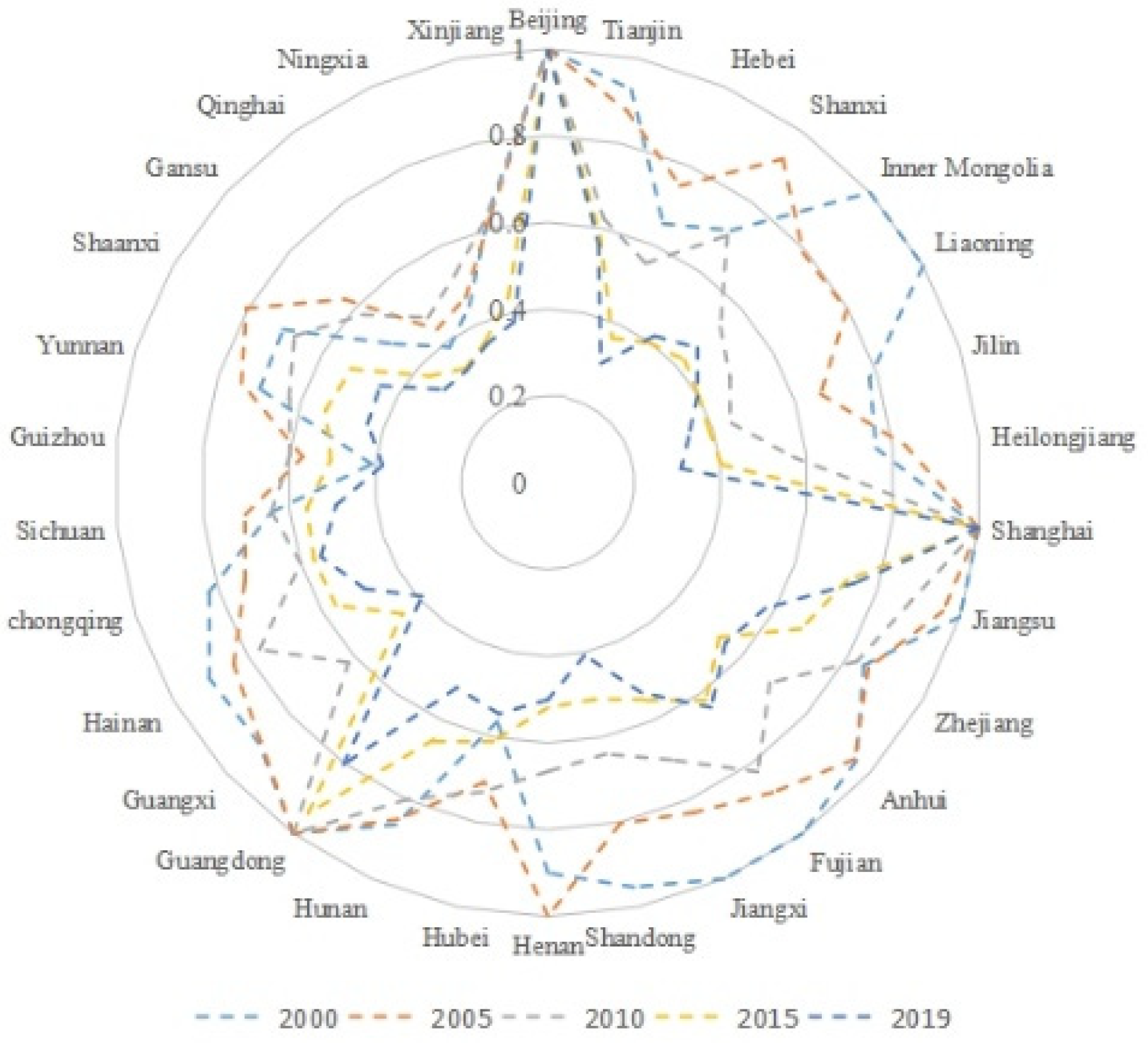
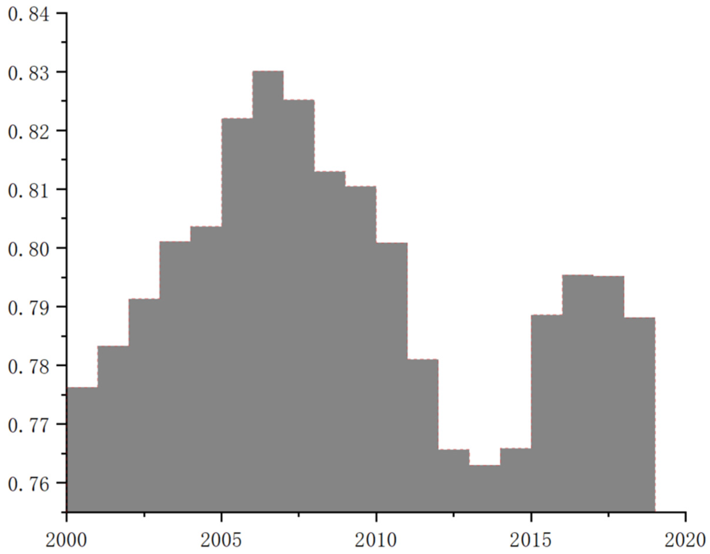
As shown in Figure 1, Beijing, Shanghai, and Guangdong have higher efficiency, while the western region is generally less efficient, with serious resource misallocation and excessive waste. The efficiency of Hebei is decreasing, which may be due to the acceptance of a large amount of outdated production capacity, resulting in low production efficiency. Meanwhile, the westward relocation of high-emission industries has also led to low efficiency in the west, among which Qinghai is the lowest. This shows that the transfer of industries cannot solve the problem of resource misallocation and excessive waste. The rectification of these backward production capacities and the development of high-tech industry are important ways to optimize resource allocation.

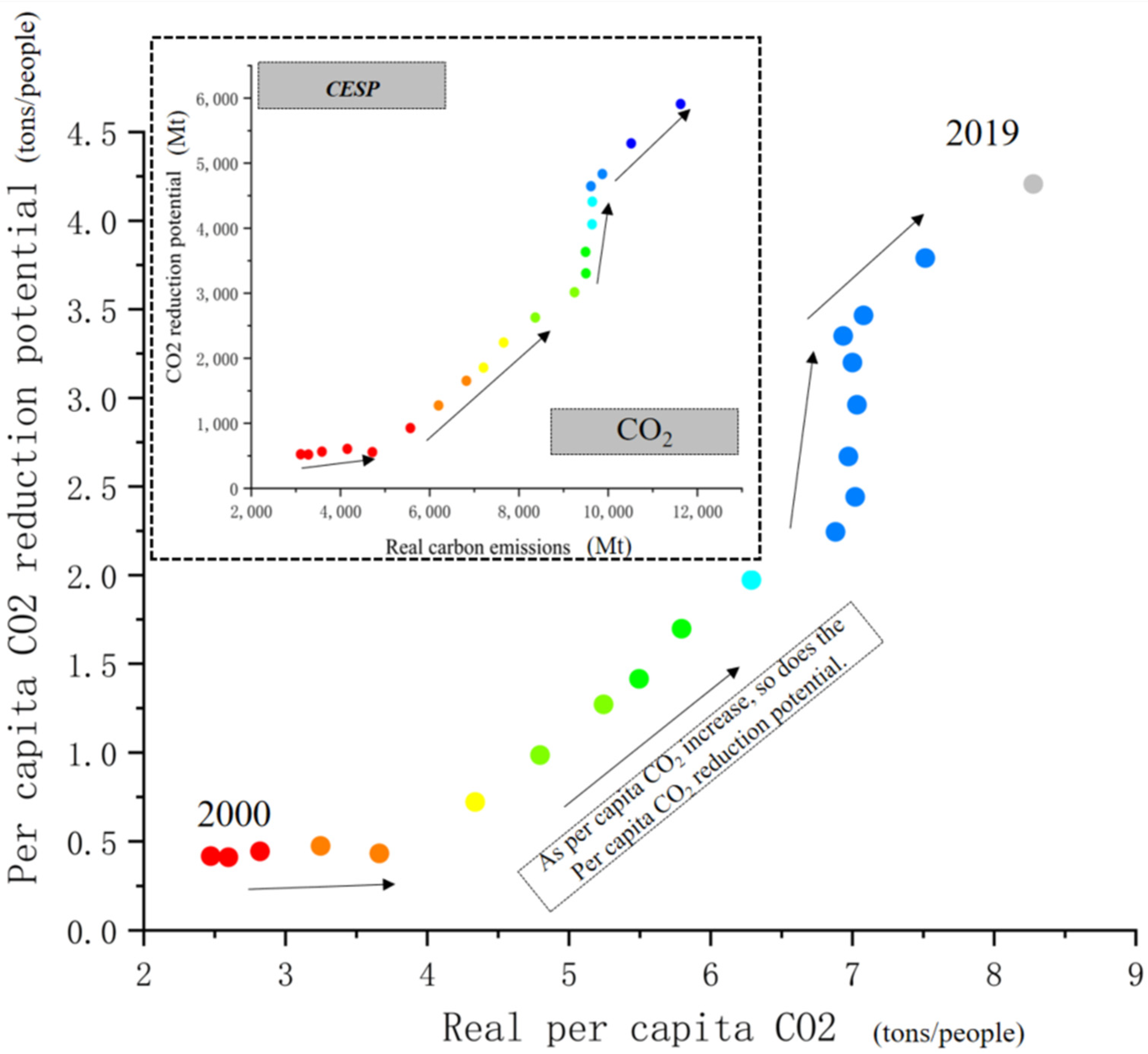
As carbon emissions increase, so does CESP. The growth of CESP can be divided into four stages: 2000–2004 (the first stage), 2005–2010 (the second stage), 2011–2016 (the third stage), and 2017–2019 (the fourth stage). From 2000 to 2004, as carbon emissions increased, CESP remained at a stable level. From 2005 to 2010, with the increase of carbon emissions, CESP also increased. From 2011 to 2016, the growth rate of CESP far exceeded the CO₂, which may be due to the misallocation of resources, resulting in low production efficiency. The fourth stage is similar to the second stage. 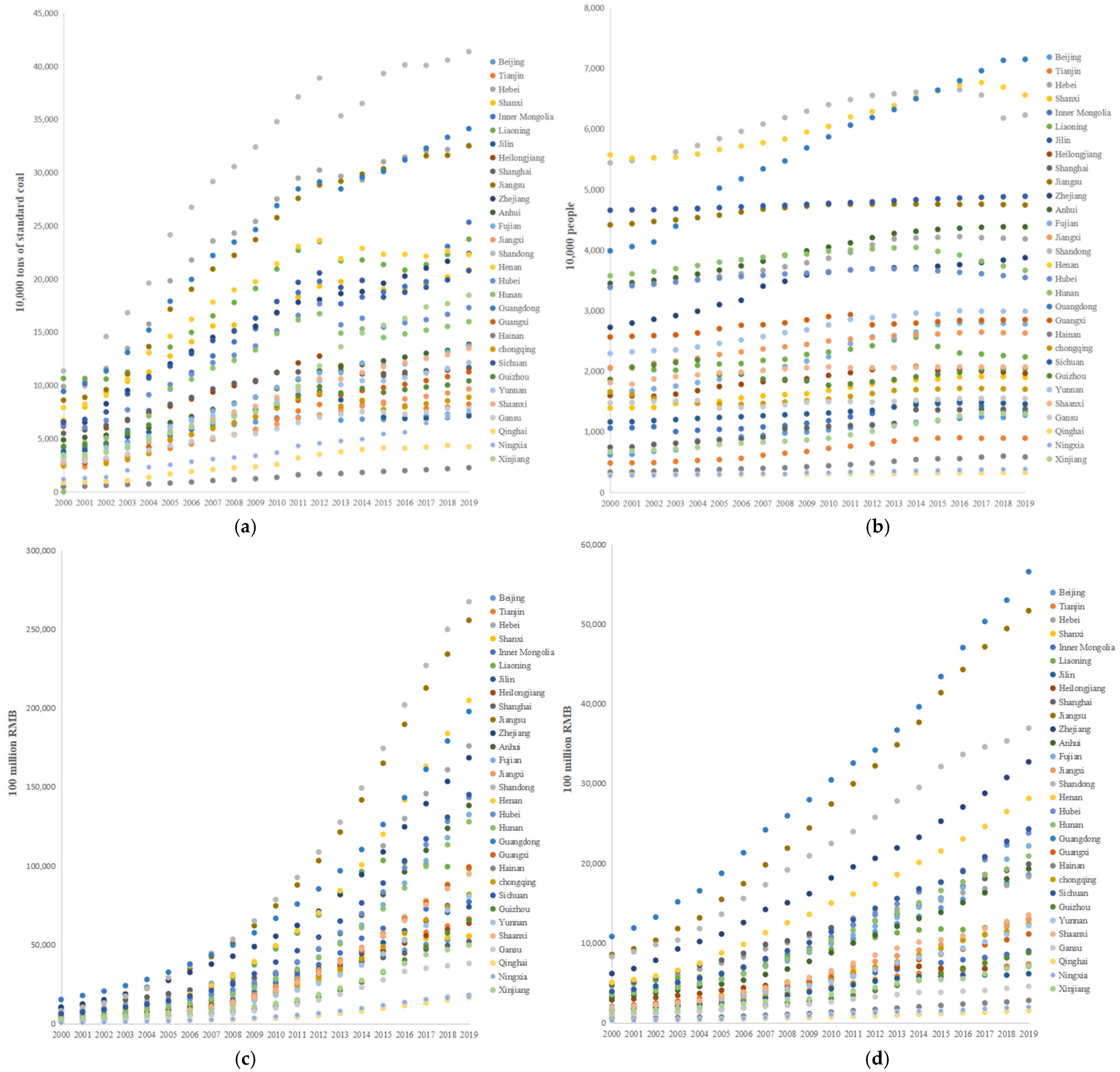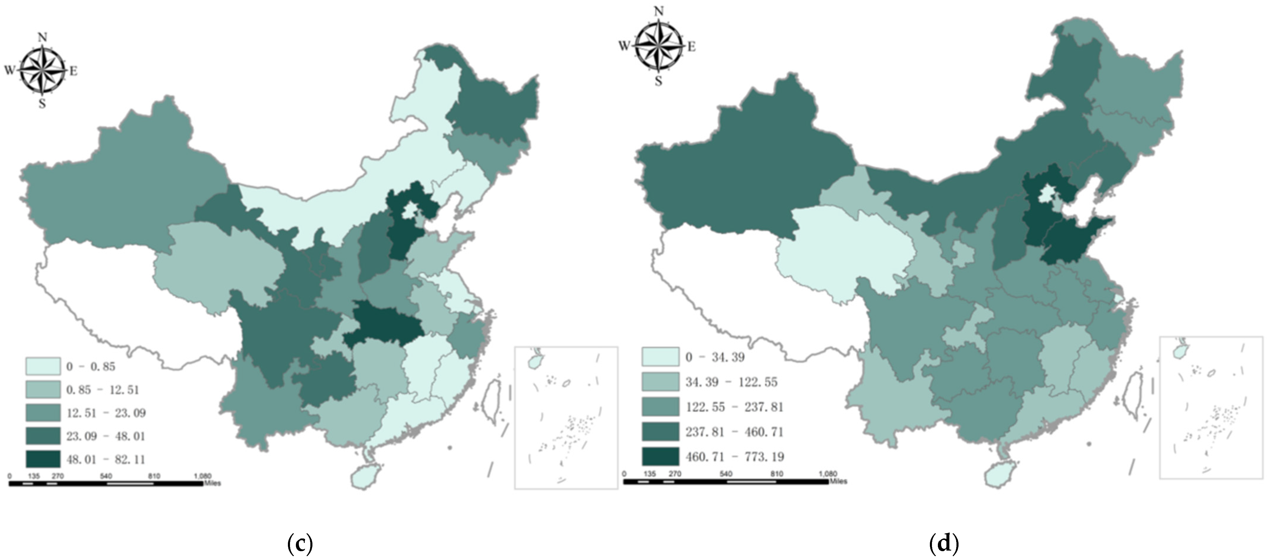As shown in Figure 2, Figure 3, Figure A3 and Figure A4, in 2000, CESP of eight provinces were zero, but in 2019, only two provinces had zero CESP, and CESP of most regions is greater than the value in 2000, which shows that with the development of the economy, the misallocation of resources is gradually increasing, resulting in excessive waste of energy.

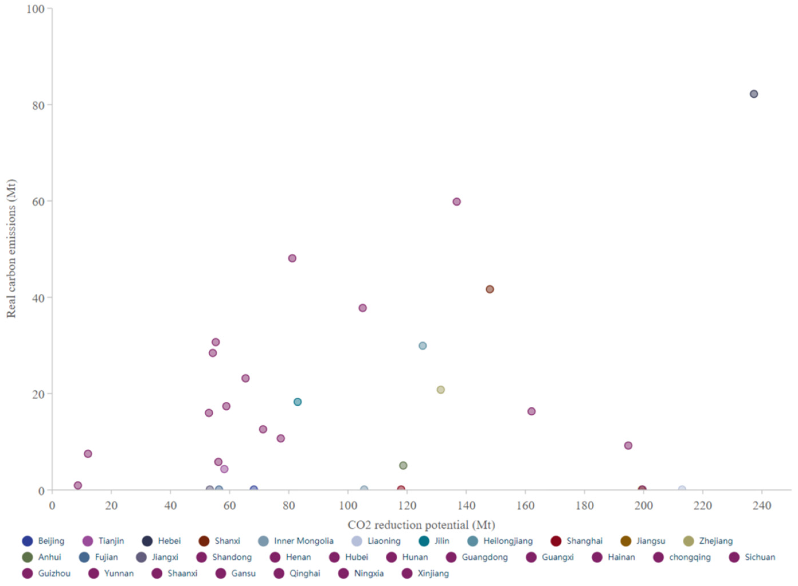
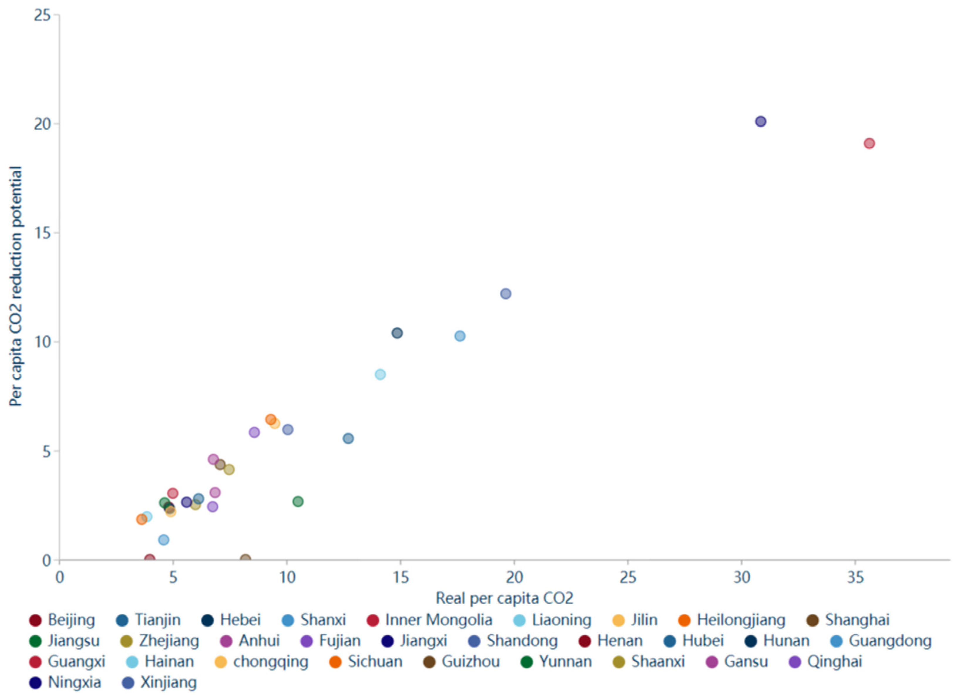
In 2000, there was no obvious relationship between CESP and CO₂, and the distribution was relatively scattered. Hebei, Shanxi, Heilongjiang, and other regions had more carbon emissions; meanwhile, CESP was also greater. However, Shandong, Liaoning, Guangdong, and other regions have high carbon emissions, but have little CESP. However, in 2019, the correlation between carbon emissions and CESP is more obvious than in 2000, among which Hebei has the largest CESP. Each province shows that with the increase in carbon emission, CESP increases. Its model R square is 0.81, and the coefficient is 0.56, which means that when carbon emission is 1 unit, the carbon emission reduction potential increases by 0.56 units. Provinces with more carbon emissions have correspondingly larger emission-reduction potentials.

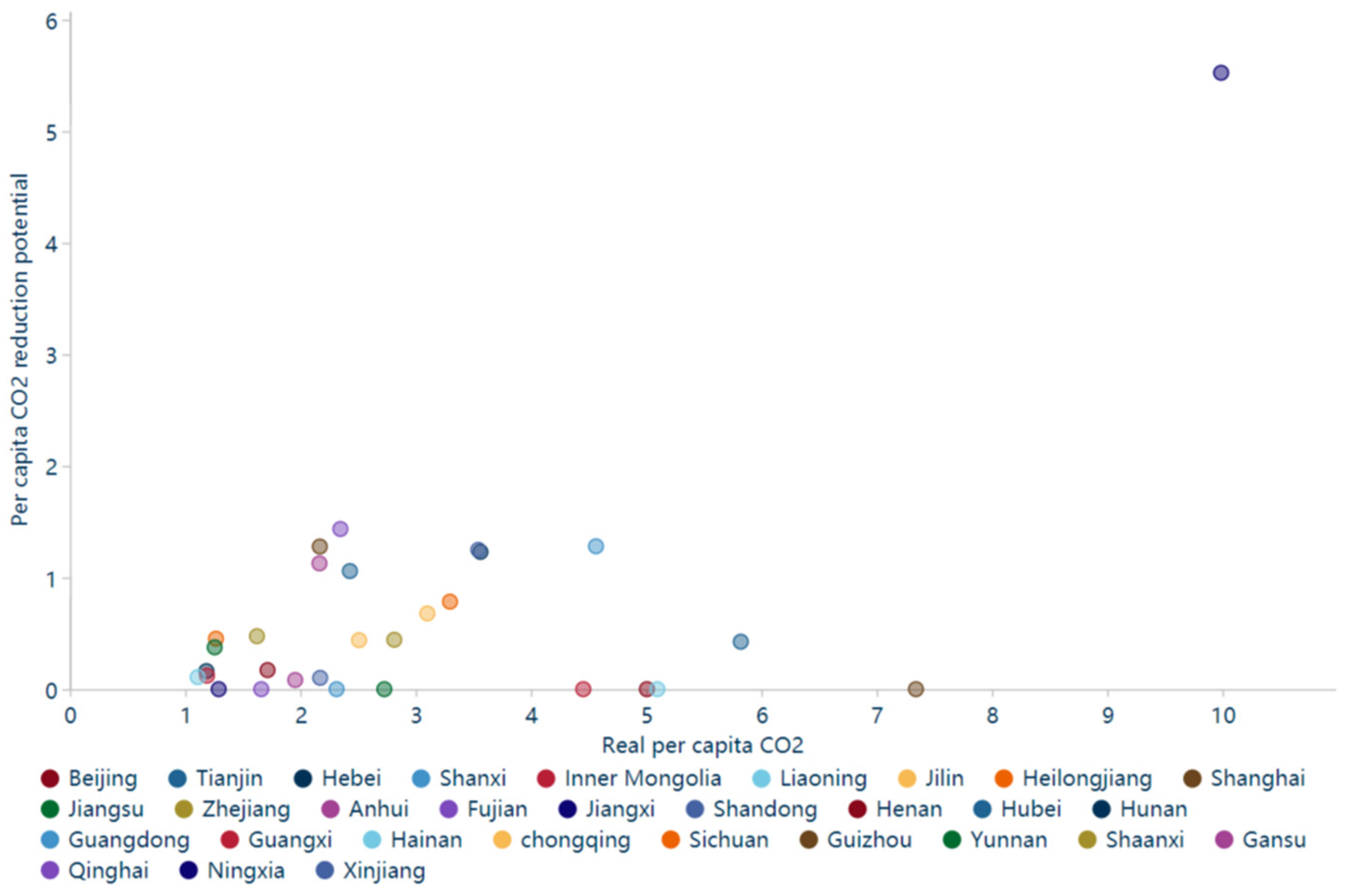
There is a strong relationship between per capita CO₂ and per capita CESP. This remarkable relationship is also divided into four stages: 2000–2004 (the first stage), 2005–2010 (the second stage), 2011–2016 (the third stage), and 2017–2019 (the fourth stage). In 2000, Hainan has the smallest per capita CESP and per capita CO₂, and Ningxia is the region with the largest per capita CESP and per capita CO₂. There was also no obvious relationship between per capita CESP and per capita CO₂, and the distribution was relatively scattered. In 2019, the per capita CESP and per capita CO₂ were lower in Beijing, and the per capita CESP and per capita CO₂ in Ningxia and Inner Mongolia are the largest. The correlation between per capita CO₂ and per capita CESP is also more obvious than in 2000. Each province shows that with the increase in per capita CO₂, the per capita CESP increases. Its model R square is 0.92, and the coefficient is 0.62, which means that when per capita CO₂ is 1 unit, the per capita CESP increases by 0.56 units.

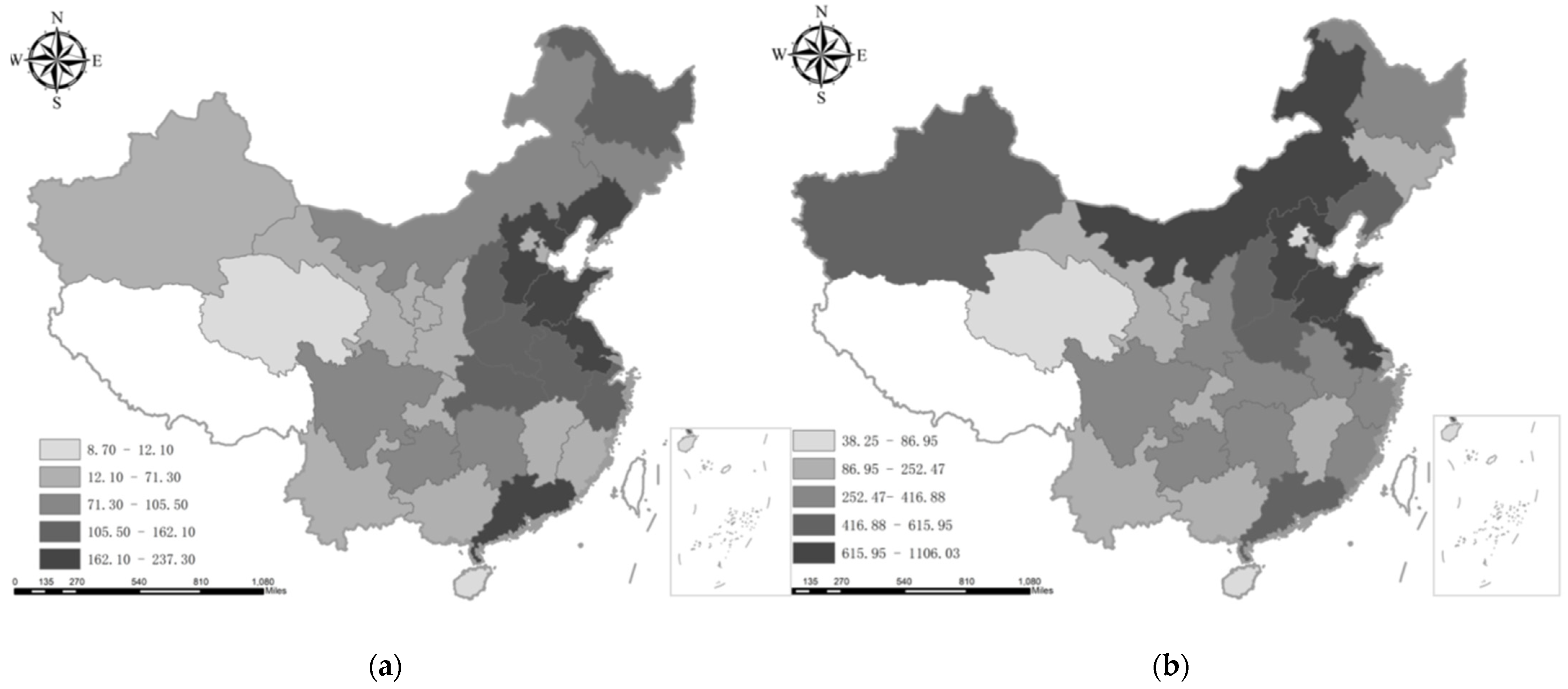
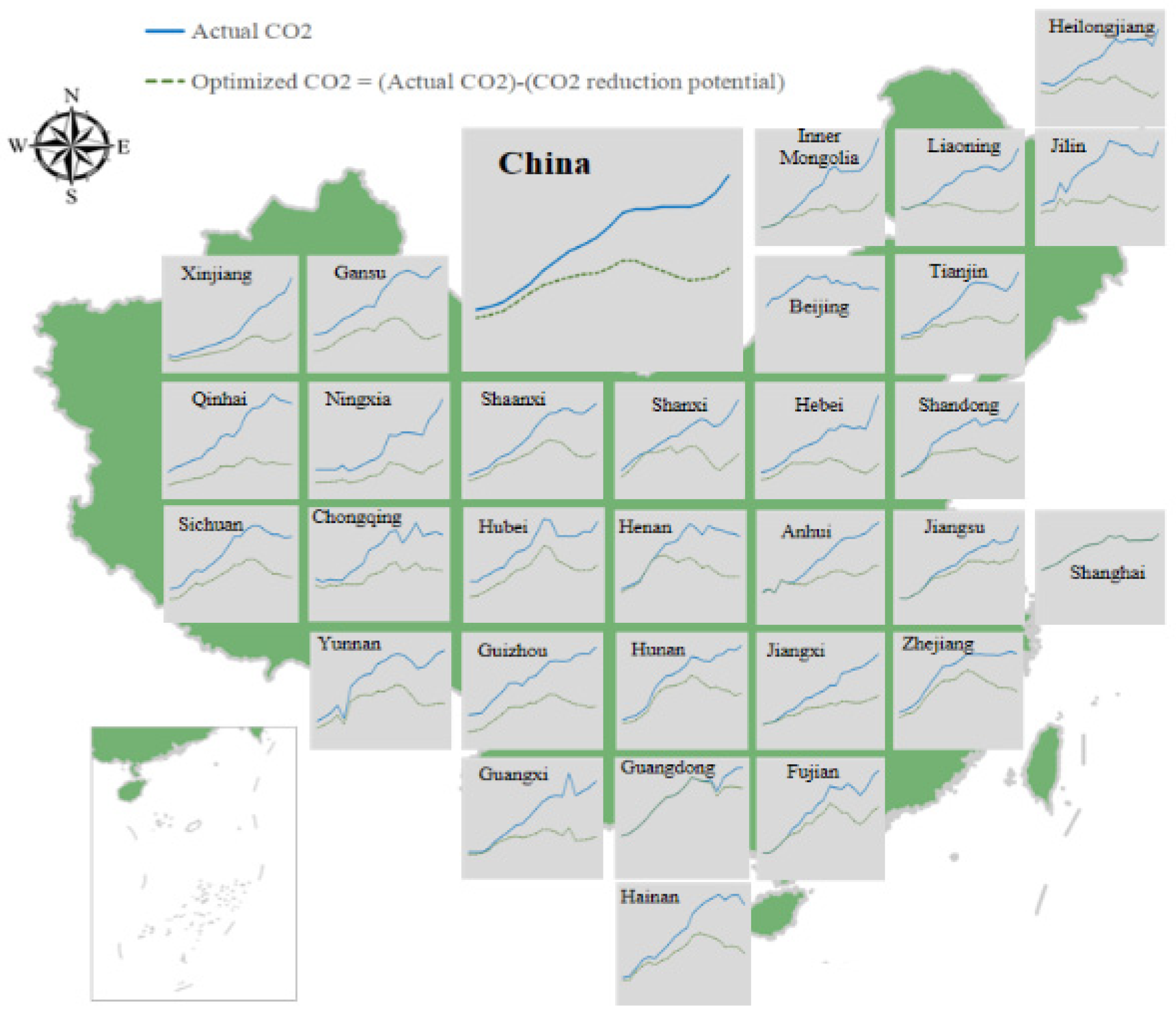
CESP is increasing, which shows that resources have not been used effectively, and there is a phenomenon of resource misallocation and waste. It can be seen from Figure 4 that the CESP of Beijing, Shanghai, and Guangdong is almost zero, which means that these regions have high resource-utilization efficiency and low emission-reduction pressure. If the CESP of the three northeastern provinces is zero, they can achieve carbon peaking before 2030, but the actual situation is that they have not reached the peak, which shows that optimizing resource allocation and improving resource utilization efficiency are of great significance for the three northeastern provinces to reach the peak. Xinjiang, Gansu, Hebei, Shanxi, Inner Mongolia, and other regions have undertaken high-energy and high-emission enterprises and output electricity roles, resulting in low resource-utilization efficiency in these regions and high CESP. There are also problems of low resource-utilization efficiency in other regions. If the resource-utilization efficiency is improved and CESP is reduced, it will promote the realization of carbon peaking and carbon neutrality as soon as possible. Hainan’s optimized carbon emissions show signs of peaking. The peak time is three years earlier than the actual situation, and the peak value is 37% lower than the actual value. The optimized carbon emissions in Zhejiang showed signs of peaking in 2013, but their actual carbon emissions have not yet peaked. The optimized peak is 26% lower than the carbon emissions in 2019. Qinghai, Sichuan, Hunan, and Guizhou can all reach their peaks earlier after the resource utilization efficiency is improved. Among them, Qinghai has the most obvious difference, and peak value is 65% lower than the actual observable peak.

3.2. Results of the Decomposition

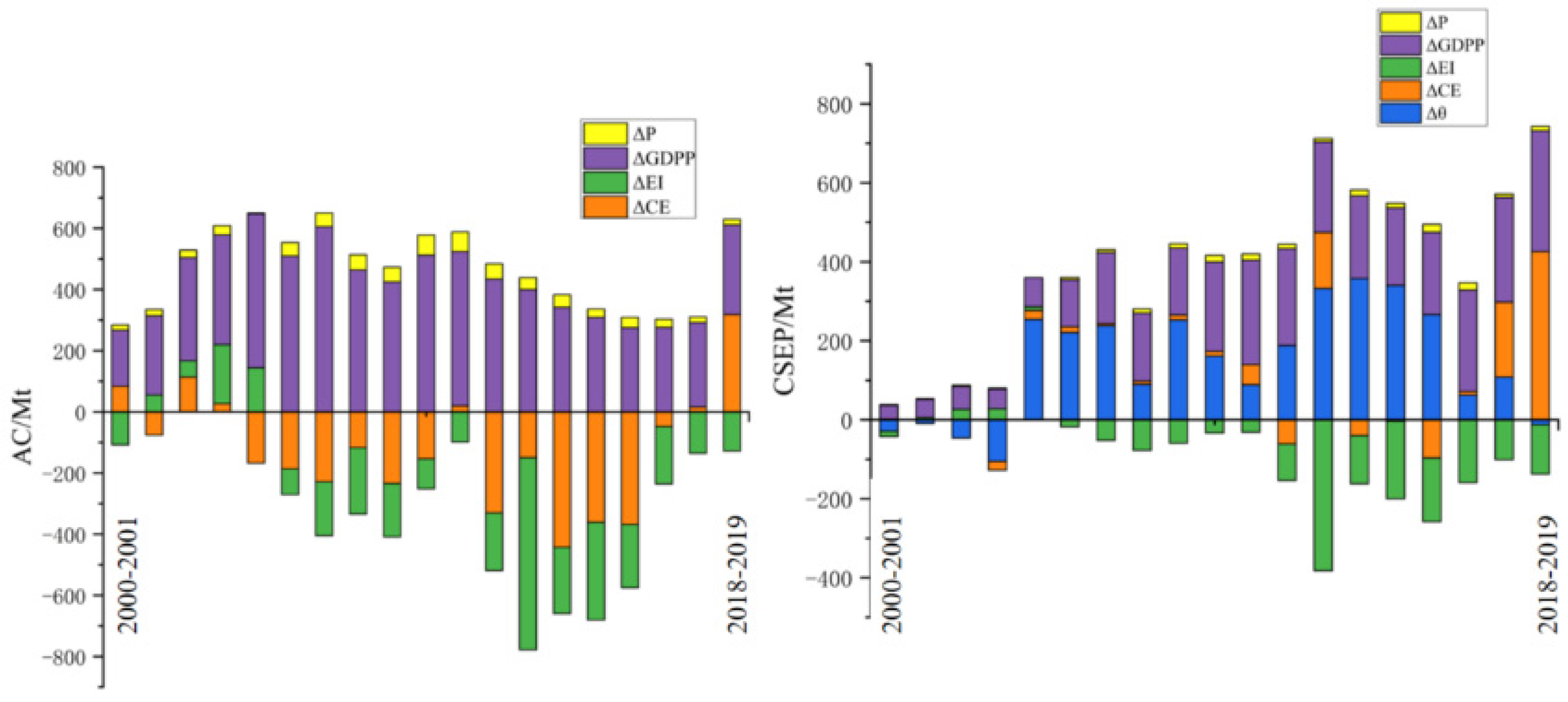
Carbon emissions are split into two parts, AC and CESP, in this paper. As shown in Figure 5, in AC, per capita GDP and population are positive contributing factors. The former is the main contributing factor, which indicates that the increase in GDP is accompanied by a large CO₂ emission, and we are not currently decoupling the economy from CO₂. However, the contribution of per capita GDP is declining, indicating that economic growth is moving toward a low-carbon direction. Energy intensity and carbon emission coefficient are negative contributing factors, and the improvement of energy utilization efficiency and energy structure restrains the increase in CO₂. In CESP, similar to AC, per capita GDP and population are still positive contributing factors. Energy intensity is the main negative contributing factor, and the contribution of the carbon-emission coefficient is more to increase CESP. Unlike AC, the change in efficiency increases CESP, indicating that resource misallocation, waste, and low utilization efficiency have increased CESP, which even exceeded per capita GDP in 2012–2016. Therefore, optimizing resource allocation and improving resource-utilization efficiency is of great significance to reduce CESP. It can be seen from the discussion in the previous section that CESP accounts for a large proportion of carbon emissions and improving resource utilization efficiency is of great significance for carbon peaking and carbon neutralization.

3.3. Spatial Correlation Analysis

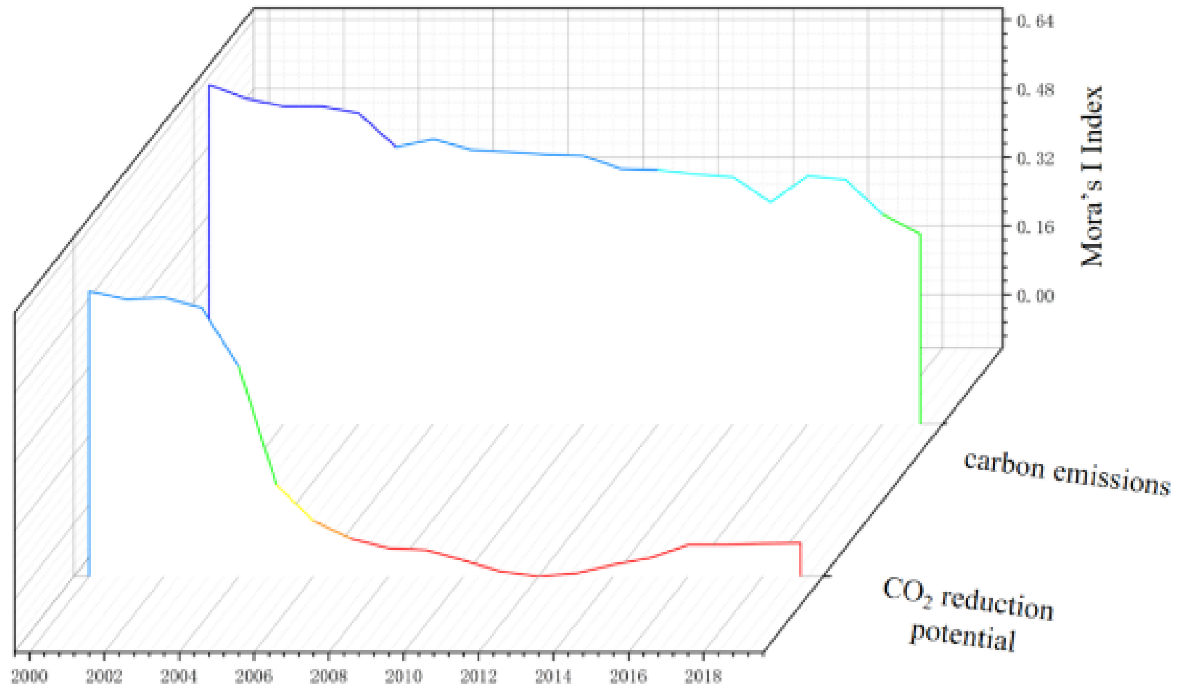
The spatial correlation analysis of CO₂ and CESP from 2000 to 2019 was carried out, employing Arcgis 10.2. According to Figure 6, CO₂ shows a strong positive correlation, and CESP also shows a coexistence of positive and negative correlations.

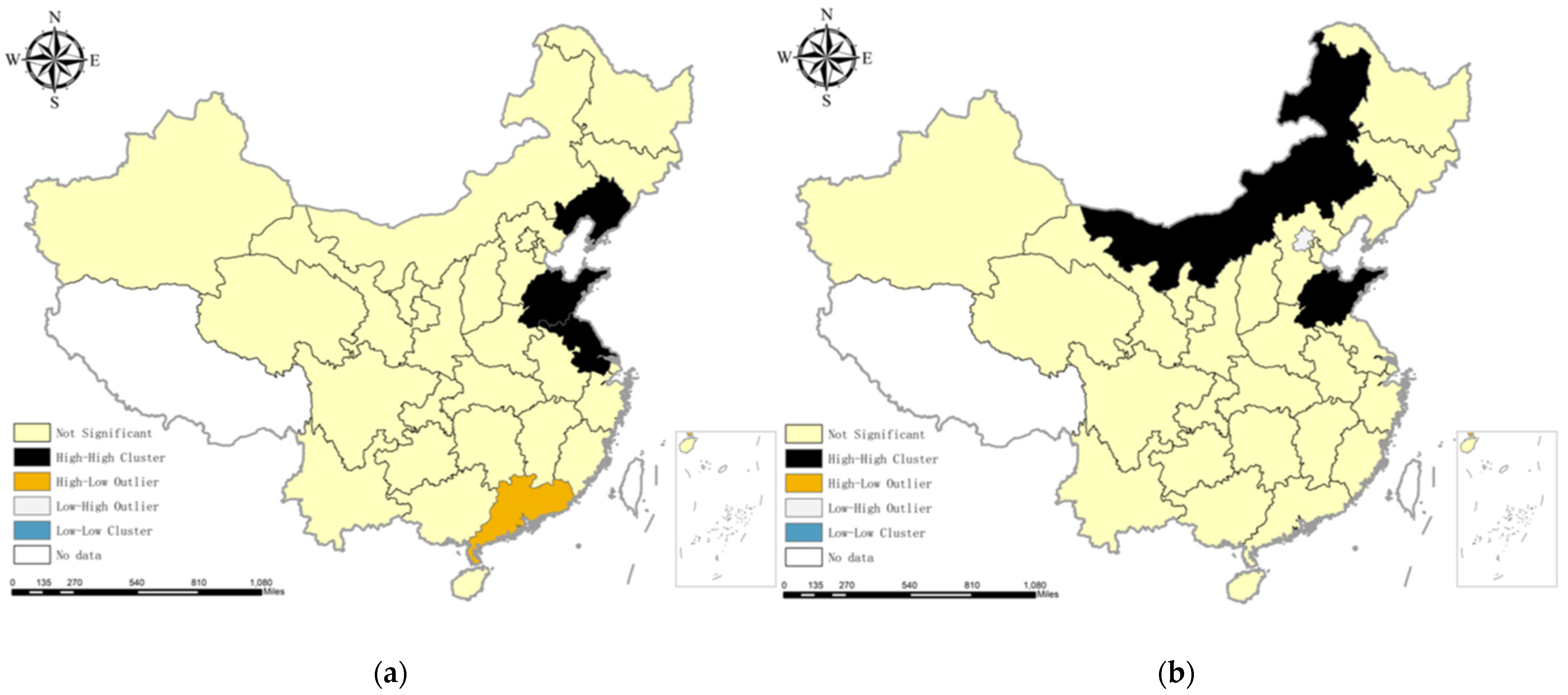
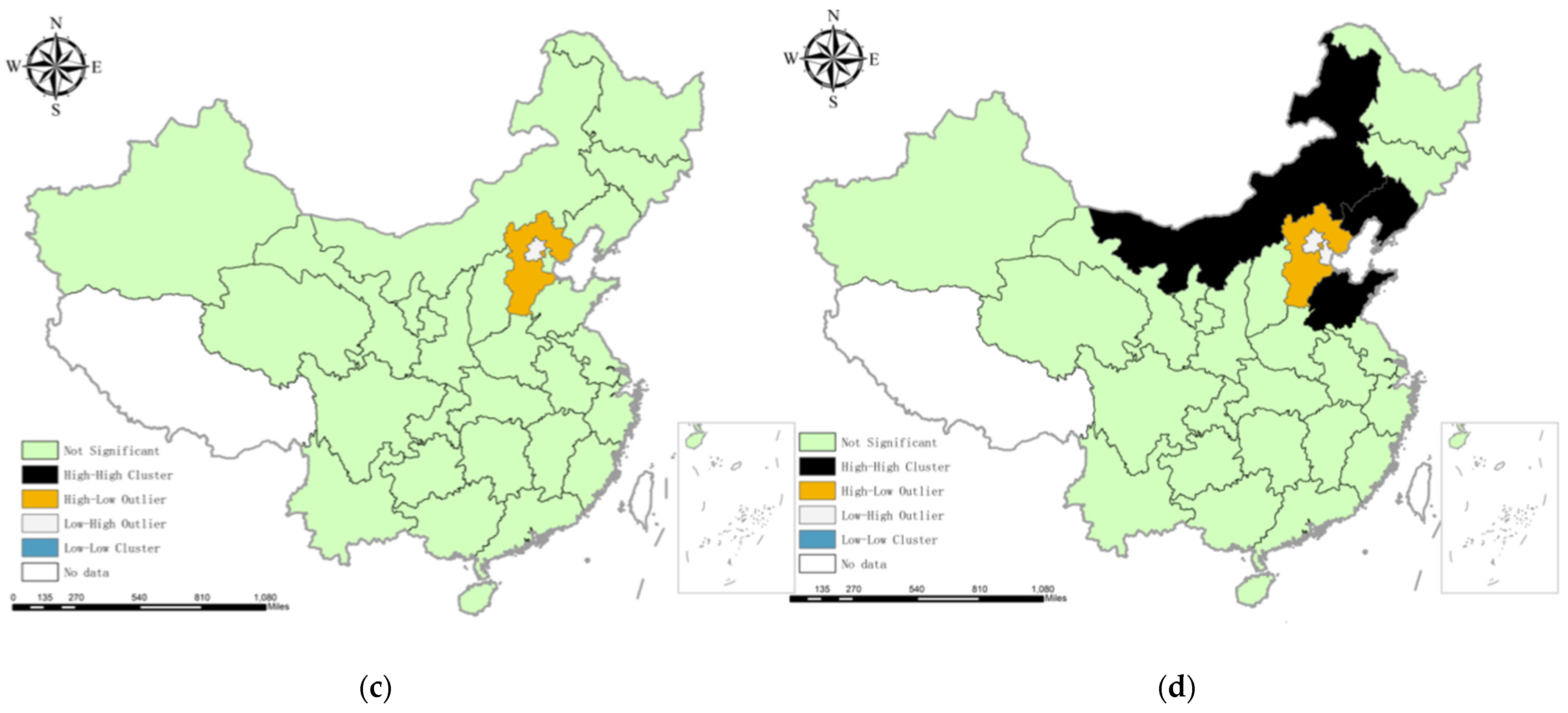
As shown in Figure 7, clustered graphs of carbon emissions and CESP are presented. In 2000, Liaoning and Shandong form high-high agglomerations, surrounded by regions with high carbon emissions. Guangdong constitutes high–low agglomerations, surrounded by regions with low carbon emissions. Hebei is a high–low agglomeration, surrounded by regions with low CESP. Beijing is a low–high agglomeration, surrounded by regions with high CESP. In 2019, Inner Mongolia and Shandong form high–high agglomerations, surrounded by regions with high CO₂. Beijing is low–high agglomerations, surrounded by regions with high emissions. Inner Mongolia, Liaoning, and Shandong form high–high agglomerations, while Beijing and Tianjin form low–high agglomerations.

3.4. Results of GTWR

The residuals of the GTWR regression results are applied to investigate the spatial autocorrelation test. According to

Table A4. The test of the residuals in GTWR.

Year	z	Year	z
2000	0.06 *	2005	0.92 *
2010	0.12 *	2015	0.36 *
2019	−0.27 *

* The significance of 0.1 has not passed.

, the spatial autocorrelations were randomly distributed, indicating that the effect was good and the reliability was high in GTWR. As shown in

Table A5. OLS of carbon emissions.

Variables (Y)	Type	R2
Carbon emissions	OLS	0.3412
	GTWR	0.9954
CESP	OLS	0.2538
	GTWR	0.9201

, the results of GTWR are significantly better than the results of OLS regression.

3.4.1. Impact of Efficiency on CO₂ and CESP

According to

Table 2. Parameters of GTWR (lnCO₂).

Variable	Min	25%	50%	75%	Max	Interquartile Range
Constant	−6.2987	−3.0215	−2.2911	−1.5365	1.4736	1.4851
lnθ	−0.8193	−0.2619	−0.1282	0.0456	0.7390	0.3075
lnEM	0.0269	0.3377	0.4909	0.6348	1.0384	0.2970
lnEI	0.3271	0.7600	0.8523	0.9545	1.3955	0.1945
lnGDPP	−0.1573	0.4797	0.5672	0.6453	1.2904	0.1656
lnP	0.1484	0.9683	1.0524	1.1555	1.3511	0.1873
lnER	−0.7148	0.1290	0.2542	0.3893	0.6457	0.2603
lnIE	−0.2938	−0.0609	−0.0272	0.0007	0.3633	0.0616
lnES	−1.4047	0.0007	0.0012	0.1386	0.8477	0.1379
lnTP	−0.6598	−0.1295	0.0470	0.2391	1.0134	0.3686
lnRL	−0.5548	−0.0841	−0.0344	0.0159	0.5243	0.1000
Adjusted R2	0.9954

and

Table 3. Parameters of GTWR (lnCESP).

Variable	Min	25%	50%	75%	Max	Interquartile Range
Constant	−69.8291	−11.6291	−3.0384	9.1692	95.1465	20.7983
lnθ	−32.4495	−11.6598	−6.8291	−4.4039	−0.6777	7.2559
lnEM	−8.6289	0.4447	1.2800	2.6514	7.3643	2.2067
lnEI	−13.2300	0.0878	1.5752	4.4420	15.3427	4.3543
lnGDPP	−12.9491	−3.0574	−0.3515	0.7904	15.6776	3.8478
lnP	−10.2223	0.3713	1.0112	1.8764	8.5833	1.5051
lnER	−8.2366	−0.3421	0.7322	4.8769	18.0334	5.2190
lnIE	−8.1196	−0.8722	0.0579	1.0525	5.9323	1.9247
lnES	−12.0808	0.7254	7.3869	11.6482	21.5458	10.9228
lnTP	−17.7582	−0.8465	0.3119	2.2410	21.7482	3.0875
lnRL	−5.5396	−0.5005	0.0700	0.6235	4.3378	1.1240
Adjusted R2	0.9201

, production efficiency can reduce both CO₂ and CESP. It is the best way to decrease CO₂ and CESP. This shows that improving resource utilization efficiency and optimizing misallocated resources are the key measures for China to achieve the dual carbon goal. The improvement of efficiency includes the optimization of resources and the advancement of technology. The optimization of resources reduces CESP. In 2019, the coefficients in Beijing, Tianjin, Hebei, Inner Mongolia, and other regions are relatively large. Hebei is −8.08, which means that the efficiency of Hebei increases by 1%, and CESP decreases by 8.08%, 62.47 Mt of CESP. The improvement of efficiency reduces carbon emissions, among which Guangdong, Guangxi, Qinghai, and other regions are the most obvious. The improvement of efficiency in some regions leads to more carbon emissions, such as in Ningxia, Shaanxi, Heilongjiang, and other regions. The impact coefficient of Shaanxi on CO₂ is 0.34, which means that the efficiency of Shaanxi increases by 1% and then CO₂ increases by 0.34%, subsequently. The degree of regulation in these regions is also weaker than that in the eastern region. Most production still employs traditional technologies in the western area. The initial profitable technology of enterprises is dirty technology, so the research and development of new technologies is not clean technology, thereby increasing CO₂ [46]. Therefore, improving the research and development of clean technologies and rectifying high-emission industries is one of the top priorities in these regions.

3.4.2. Impact of Energy Mix on CO₂ and CESP

From Table 2 and Table 3, it can be seen that the deterioration of the energy mix (increase in coal consumption) in each region has a positive impact on CO₂ and CESP, and greater CESP hinders China from achieving the dual carbon goal. The impact of the coal proportion in each province on carbon emissions has decreased. This is because the state has made significant contributions to develop clean energy and reduce coal consumption, resulting in the marginal impact of coal proportion gradually decreasing. In 2019, the proportion of coal has a greater impact on CO₂ in the western region. Xinjiang is 0.63, which means that the proportion of coal in Xinjiang is reduced by 1%, and carbon emissions are reduced by 0.63%. Xinjiang has received high-emitting industries from the eastern region, resulting in an increase in local CO₂. Meanwhile, due to the increase in the power transmission from Xinjiang to the east, carbon emissions from other regions have also been transferred to Xinjiang. In 2019, in Shandong, located in the eastern region, the proportion of coal has a positive impact on CESP, and the coefficient is the largest, 3.17, which means that the coal proportion is reduced by 1%, and CESP is reduced by 3.17%. Shandong is an economically developed province, but its development model is accompanied by high energy consumption and high CO₂. With the development of industrialization and urbanization, secondary industry is developing rapidly, which creates more demand for energy. Meanwhile, coal accounts for a large proportion in Shandong [47]. On the whole, differences are obvious in the impact of coal proportion on CO₂ and CESP. The regions with greater impact on CO₂ are concentrated in the west and some eastern regions dominated by fossil energy, and the regions with a greater impact on CESP are concentrated in the central and eastern regions. Therefore, all regions should appropriately control coal consumption.

3.4.3. Impact of Energy Intensity on CO₂ and CESP

According to Table 2 and Table 3, it can be seen that the increase of utilization efficiency in energy will reduce carbon emissions and CESP. In 2019, energy intensity had a greater impact on CO₂ in Inner Mongolia, Shanxi, and Hebei, with Inner Mongolia being the largest, meaning that Inner Mongolia’s energy intensity decreased by 1% and carbon emissions decreased by 1.17%. The CESP of Jiangsu, Zhejiang, Inner Mongolia, and other regions is greatly affected by energy intensity, of which Jiangsu is 3.84. However, the reduction of energy intensity in Shandong, Henan, Guangdong, and other regions will increase CESP, of which Guangdong is −9.2%. Meanwhile, Xu [48] believes that high efficiency in energy may trigger rebound effects and increase energy consumption and lead to excessive energy input, resulting in diminishing returns to scale, misallocation, and congestion of resources, and finally increase CESP.

3.4.4. Impact of Per Capita GDP and Urbanization Rate on CO₂ and CESP

According to Table 2 and Table 3, the impact of per capita GDP on CO₂ is positive, which indicates that rapid economic growth will be accompanied by an increase in CO₂. The coefficients, except in the eastern regions, increase, indicating that although the economies of these regions have developed, they also generate more CO₂ because of production structures. In 2019, the coefficients in Inner Mongolia, Liaoning, Shanxi, Hebei, Xinjiang, and other regions are relatively large, among which Heilongjiang is 1.03, which means that a 1% increase in per capita GDP in Heilongjiang will increase carbon emissions by 1.03%. Interestingly, the per capita GDP has a negative impact on CESP, which means that economic growth reduces CESP. Moreover, the government and enterprises have more economic strength to develop and research new technologies and new energy. The coefficients in Jiangsu, Zhejiang, and Shandong are relatively large, indicating that although the economic development of these regions has increased carbon emissions, it has reduced CESP and promoted the improvement of resource utilization efficiency. The economic development of Inner Mongolia and other regions will increase CESP, with a coefficient of 3.27, which means that a 1% increase in per capita GDP increases CESP by 3.27%.

According to Table 2 and Table 3, the impacts of urbanization development on CO₂ and CESP are both positive. It shows that although the transfer of urban population promotes urbanization and industrialization, it also brings tremendous environmental pressure, more energy consumption, and more CO₂. The urbanization development of some regions, such as Beijing, Tianjin, Shandong, and other regions, will reduce CESP. This is because the urbanization process in these regions promotes the concentrated consumption of resources and improves energy efficiency, decreasing CESP. In 2019, Beijing’s coefficient was −0.97, meaning that Beijing’s urbanization rate increased by 1% and its CESP decreased by 0.97%.

3.4.5. Impact of Electrification Rate on CO₂ and CESP

According to Table 2 and Table 3, the increase in the electrification rate in most regions will increase carbon emissions and CESP. The energy consumption accelerates economic development; meanwhile, power generated by fossil-fuel energy still occupies a large proportion. The implementation of measures such as coal-to-electricity conversion has further aggravated the demand for electricity, and the high proportion of coal-fired electricity has resulted in the ineffectiveness of the increase in the electrification rate on CO₂ reduction. Meanwhile, measures, such as low electricity prices and the sending of appliances to the countryside, have led to greater demand for electricity, thereby curbing the contribution of electrification rates to carbon emission reductions. However, the coefficients in Shanghai, Zhejiang, Guangdong, Qinghai, and other regions are negative, meaning that increasing the electrification rate will reduce carbon emissions. Shanghai, Zhejiang, Guangdong, and other regions are mostly recipients of externally transferred electricity. Moreover, these provinces are also vigorously developing clean energy, resulting in a significant effect on CO₂ reduction because of the increase in the electrification rate. The electrification rate in Qinghai, a vigorous development of clean electricity, has the greatest impact on carbon emission reduction; that is, the electrification rate increases by 1%, and the carbon emission decreases by 0.39%. The electrification rate has a positive impact on CESP, which means that the electrification, based on thermal power, has not reduced CESP because electricity has energy loss in the process of processing and conversion. If the proportion of thermal power in electricity is high, electrification cannot improve energy efficiency. However, the increase in the electrification rate in Qinghai, Yunnan, and other regions will reduce CESP because these regions are mainly dominated by clean energy sources. In 2019, Qinghai’s influence coefficient was −0.33, meaning that a 1% increase in the electrification rate would reduce its CESP by 0.33%.

3.4.6. Impact of Trade on CO₂ and CESP

According to Table 2 and Table 3, trade reduces carbon emissions and CESP. Import trade can reduce carbon emissions through technological spillovers and environmental regulations, and export trade can reduce carbon emissions through structural and scale effects [49]. Meanwhile, foreign trade has also improved the efficiency in the resource and removed excess capacity in production. However, there is “pollution refuge” in some regions, such as Guangdong, Guangxi, Xinjiang, Ningxia, and other regions. The products produced are accompanied by high energy consumption in trade. In 2019, Xinjiang’s imports and exports had a relatively large impact coefficient on carbon emissions, which was 0.11, meaning that an increase of 1% in trade would increase carbon emissions by 0.11%. Regarding the CESP, the trade of Shandong, Hebei, Liaoning, and other regions will increase the CESP. Although the trade will reduce carbon emissions in these regions, more trade output will lead to greater CESP in the case of resource misallocation and waste. Therefore, it is of great significance to adjust the import and export trade structure and optimize the allocation of resources to achieve the dual carbon goal.

3.4.7. Impact of Economic Structure on CO₂ and CESP

From Table 2 and Table 3, the increase in the proportion of secondary industry will increase carbon emissions and CESP. The increase in the proportion of secondary industry will increase the demand for energy, thereby increasing carbon emissions. Meanwhile, resource-intensive industries can lead to low energy efficiency and high carbon intensity, thereby increasing CESP. Heilongjiang, Jilin, Liaoning, and other regions have large coefficients, indicating that these regions are key areas for industrial restructuring. Among them, the proportion of secondary industry in Heilongjiang will decrease by 1%, and then carbon emissions will decrease by 0.49%. The CESP of the eastern region is most affected by the industrial structure, indicating that the optimization and upgrading of the industrial structure has obvious potential for reducing CESP in the eastern region. Among them, the coefficients of Jiangsu and Shandong are the largest, which are 21.55 and 19.30, respectively. That is, the proportion of secondary industry decreases by 1%, and then CESP decreased by 21.55% and 19.30% respectively. The coefficient in Qinghai is low, indicating that carbon emissions and economic output in these regions are low. The increase in the proportion of industry will increase the demand for energy, and, meanwhile, it will also update local backward equipment to improve production efficiency.

3.4.8. Impact of Climate Conditions on CO₂ and CESP

From Table 2 and Table 3, climate conditions have relatively little impact on carbon emissions and CESP. Higher temperature and lower precipitation have a greater impact on carbon emissions and CESP. In areas with a favorable climate, energy consumption in terms of comfort will be less than in areas with harsh climates. High temperature will frequently cause people to use refrigeration devices such as air conditioners, and low precipitation will increase energy consumption to meet water supply. The impact of climatic conditions in the western region on carbon emissions is greater than that in the central and western regions. Shaanxi, Ningxia, and other regions are more obvious. In 2019, a 1% increase in temperature and a 1% decrease in precipitation increased carbon emissions by 0.46% and 0.16%, respectively. The deterioration of climatic conditions has a greater impact on CESP in the central and eastern regions, and Henan is the most obvious. A 1% increase in temperature and a 1% decrease in precipitation will increase CESP by 2.9% and 2.26%, respectively.

4. Conclusions

This paper explores the factors of CO₂ from the perspective of CESP. Employing the data of 30 provinces from 2000 to 2019, combined with DEA, index decomposition, and the GTWR model, the CESP in each region and the influencing factors are explored. Then, we provide a policy reference for achieving carbon peaking and carbon neutrality goals as soon as possible.

The changes of CESP can be divided into four stages. From 2017 to 2019, the per capita CESP of each province showed a strong correlation with per capita carbon emissions. If carbon emissions increase by 1 unit, the CESP will increase by 0.56 units. Hainan, Zhejiang, Qinghai, Sichuan, Hunan, and Guizhou can reach the peak earlier when the efficiency is optimal, and the peak value is lower than the actual carbon emission. Among them, Qinghai is 65% lower than the actual observed peak.

Carbon emissions can be composed of AC and CESP. In AC and CESP, per capita GDP and energy intensity are the main positive factor and negative factor, respectively. The impact of efficiency changes on CESP is mostly positive, even exceeding the combined contributions of per capita GDP and population in 2012–2016, but after that the impact of efficiency gradually diminishes.

When analyzing the results of the GTWR, we found that the improvement of efficiency, the reduction in coal proportion and energy intensity and the increase in trade will reduce CO₂ and CESP. Per capita GDP increases CO₂ but reduces CESP. Therefore, it is still very important to deal with the problem between the economy and the dual carbon goals. The increases in the urbanization rate and electrification rate will increase CO₂ and CESP.

Efficiency is the most influential factor affecting the CESP, among which Hebei is −8.08; that is, a 1% increase in efficiency can reduce the CESP of 62.47 Mt. The effect of energy intensity reduction on CO₂ and CESP in Inner Mongolia is obvious. Economic development and the increase in the urbanization rate are more effective in reducing the CESP of the eastern region. In areas with a high proportion of clean energy power, the impact of the electrification rate is negative. In 2019, a 1% increase in the electrification rate in Qinghai will reduce the CESP by 0.33%. The phenomenon of a “pollution shelter” exists in Xinjiang, Guangxi, Guangdong, and other regions, but trade will reduce CESP.

This paper employs DEA-IDA to explore CESP in 30 regions. The CESP takes the current production frontier as the standard and uses input and output to describe the gap between each DMU and the production frontier. This method is difficult for conducting detailed research on the impact of relevant policies. In future research, we will embed the policy impact into the model to more comprehensively study the real situation of DMU.

According to the conclusions obtained in this paper, we propose some policy implications.

The government should improve the efficiency of resource utilization and introduce advanced technology. Efficiency is the biggest factor affecting the CESP. Increasing resource utilization efficiency can not only improve production efficiency and avoid excessive waste, but also realize the “dual carbon” goal. It is one of the important measures to achieve the decoupling of CO₂ and the economy. The government should also abandon outdated production technology and improve research and development of clean technology.

The government should improve the energy mix, increase clean energy consumption, and reduce carbon emissions and CESP from the source. Meanwhile, improvement of the energy mix can also release the dividend of the effect of the electrification rate, since the current electrification rate dominated by thermal power has little effect on carbon emission reduction. After the electricity is clean, the improvement of the energy structure can not only reduce CO₂ and CESP, but also further exert a greater effect through the promotion of the electrification rate.

The state should develop clean products in trade and reduce the increase in CO₂ at the source. We also should develop high-tech products, adjust the structure of export commodities, increase the export of knowledge-intensive or technology-intensive products, and avoid becoming a “sanctuary of pollution”. Meanwhile, the construction of the carbon market should be improved to force enterprises to improve energy efficiency and reduce emissions.