Compound Positioning Method for Connected Electric Vehicles Based on Multi-Source Data Fusion

Abstract

With the development of electrified transportation, electric vehicle positioning technology plays an important role in improving comprehensive urban management ability. However, the traditional positioning methods based on the global positioning system (GPS) or roadside single sensors make it hard to meet requirements of high-precision positioning. Considering the advantages of various sensors in the cooperative vehicle-infrastructure system (CVIS), this paper proposes a compound positioning method for connected electric vehicles (CEVs) based on multi-source data fusion technology, which can provide data support for the CVIS. Firstly, Dempster-Shafer (D-S) evidence theory is used to fuse the position probability in multi-sensor detection information, and screen vehicle existence information. Then, a hybrid neural network model based on a long short-term (LSTM) framework is constructed to fit the mapping relationship between measured and undetermined coordinates. Moreover, the fused data are proceeded as the input of the hybrid LSTM model, which can export the vehicular real-time compound positioning information. Finally, an intersection in Shijingshan District, Beijing is selected as the test field for trajectory information collection of CEVs. The experimental results have shown that the uncertainty of fusion data can be reduced to 0.38% of the original level, and the maximum error of real-time positioning accuracy is less than 0.0905 m based on the hybrid LSTM model, which can verify the effectiveness of the model.

1. Introduction

With the development of the electric vehicle industry in recent years, intelligent connected electric vehicles (CEVs) have become one of the choices for traveling. Compared with the internal combustion engine vehicle, there are characteristics of the real-time acquisition of vehicular data, energy transmission efficiency, and the accuracy of vehicular speed control, which leads to the suitableness of electric vehicles in real-time high-precision compound positioning [1,2,3]. The high-precision and robust information of vehicular positioning can not only work for the navigation, but also provide the data support for the perception, decision-making, and path planning modules in CEVs [4,5,6]. However, it is hard to meet the requirements of high-precision perception though any single sensor in real complex traffic environments [7,8,9].

Multi-sensor fusion is a technology that comprehensively processes and optimizes the acquisition, representation, and internal relationships of various kinds of information, which is widely used in object positioning. With the improvement of lidar hardware accuracy, multi-sensor fusion is gradually applied in the compound positioning of CEVs. Moreover, the data of different spatiotemporal dimensions collected by a sensor, which is mounted on the roadside, can be provided to CEVs through the V2X units [10,11]. The accurate data perceived from compound positioning can be used as the data support and the theoretical basis for optimizing the functions of traffic flow analysis [12,13], traffic flow forecasting, and travel time reconstruction.

With the rapid development of the cooperative vehicle-infrastructure system (CVIS), the compound positioning technology of CEVs was widely studied due to its high accuracy, high reliability, and ultra-low latency [14,15]. Watta et al. [16] presented an intelligent system based on V2V communication, which combined the synergy of neural networks and geometric modeling. The model extracted the key geometric features as the input of a trained neural network to detect and predict remote vehicular positions. Song et al. [17] proposed a novel framework of a blockchain-enabled vehicle to everything (V2X) with compound positioning for improving the vehicular global positioning system (GPS) positioning accuracy, system robustness, and security. A self-positioning correction scheme for the CEV was proposed to improve their positioning accuracy, which used the multi-traffic signs as benchmarks to correct the vehicular position by a deep neural network (DNN) algorithm. Kim et al. [18] proposed an intelligent position-tracking control algorithm for vehicles considering actuator (DC motor) dynamics. The proposed controller formed the conventional multiloop structure including disturbance observers for each loop. Jung et al. [19] proposed a compound method for target classification based on evidence theory and the fuzzy logic method to achieve target localization by fusing data obtained from cameras and radar sensors. Ye et al. [20] proposed a two-stage Kalman filter algorithm, which employed two intertwined filters for channel tracking, position tracking, and abrupt channel change detection. Ko et al. [21] achieved vehicular positioning by applying V2X, which was helpful to realize autonomous driving. Caltagirone et al. [22] proposed a cross-fusion algorithm based on lidar and camera data to detect vehicle targets on the road. The results showed that the performance of the cross-fusion classification was better by comparing the performance difference between one layer and all layers. Golestan [23] proposed an advanced information fusion framework based on a multi-entity Bayesian network, which could be used in dangerous driving state identification of CEVs. This method improved the safety performance of vehicles greatly. Mostafavi et al. [24] regarded that GPS could be used as a supplement to radio-based positioning techniques and proposed the combination of distance and angle measurements with vehicle acceleration measurements to generate position estimates. In order to accurately position wheeled vehicles in GPS-deprived scenarios, Onyekpe et al. [25] proposed a wheel odometry neural network (WhONet) to learn and correct the uncertainty in wheel speed measurement required for accurate positioning by adopting the deep learning method.

In addition, in the research of compound positioning by multi-source data, it is necessary to consider the working characteristics of different sensors and the complementarity of applicable scenarios [26]. In addition, the compound positioning of CEVs in simple scenarios can be achieved through the global navigation satellite system (GNSS), and GNSS is not effective for intersection scenarios with poor signals and complex environments [27,28]. At present, many scholars have considered the research on the fusion of compound multi-source data and applied it to various traffic scenarios for CEVs. Altoaimy et al. [29] proposed a positioning method based on fuzzy logic, which included the signal-to-noise ratio (SNR) in the determination of weight factors. The method was evaluated in several simulation scenarios with different vehicle numbers, with positioning errors ranging from 0.85 m for 20 vehicles to 0.25 m for 200 vehicles. Escalera et al. [30] proposed a multi-sensor data fusion method based on the global nearest neighbor algorithm for vision system, laser sensors, and GPS, which was used for safe vehicular detection on single-lane roads. This method overcame the limitations of single sensors and provided reliable safety for traffic applications. Broughton [31] established a multi-sensor fusion system for detecting pedestrians in conditions of foggy weather, which improved the accuracy of fused data in dynamic and unknown environments. The experiments indicated that in the event of the loss of information from a sensor, pedestrian detection and position estimation were still effective. Mo et al. [32] proposed a compound positioning framework of information fusion for CEVs and roadside infrastructure, which provided a solution for fusion between CEVs, intelligent infrastructure, and intelligent control systems. Xiao et al. [33] developed a unified theoretical framework for multiple-target positioning by fusing multi-source heterogeneous information from the on-board sensors and V2X technology. Meanwhile, the integrity of target sensing was significantly improved by the sharing of multi-source data and development of map data. Kim et al. [34] proposed a particle filter fusion algorithm based on information entropy theory, which integrated multi-layer vertical features and road intensity features of maps in different periods for precise vehicular positioning in urban traffic. With the gradual development of deep learning, positioning methods based on neural networks brought better results. Onyekpe et al. [35] analyzed the performance of long short-term memory (LSTM), input delay neural networks (IDNN), multi-layer neural networks (MLNN), and the Kalman filter for high data rate positioning and have shown that deep neural network-based solutions could have better performances. The combination of neural networks and communication technology in autonomous driving will further improve the robustness and accuracy of positioning.

Based on the above research, it can be summarized that there are two aspects of research gaps:

• In the research of roadside-based traffic perception, the current studies mainly focus on the dynamic detection of vehicles with single sensors on the roadside;
• In the compound positioning research of vehicles, the current studies mainly focus on the multiple sensors of a single vehicle, and there is a gap in the cooperative compound positioning of multiple vehicles based on vehicle-infrastructure information fusion.

In conclusion, with the rapid development of the CVIS, CEVs on the road perceive their own position dynamically based on roadside multi-source data fusion technology, realizing the positioning function [36]. Meanwhile, the vehicle on the road can be represented as independent nodes, which continuously communicate with other nodes, roadside units, and mobile devices in real time [37]. The system applied proposed method can realize the compound positioning perception of the vehicles and improves the safety of driving as well as the road traffic capacity.

This paper aims to study CEVs and vehicle-infrastructure information fusion technology, proposing a method based on a hybrid neural network model to realize real-time perception of vehicular compound positioning. The main contributions of this paper can be summarized as follows:

• A comprehensive system concept is provided based on the positioning accuracy requirements of CEVs.
• A reliable compound positioning approach is developed to achieve higher positioning accuracy among the data obtained from multiple roadside sensors and V2X units.
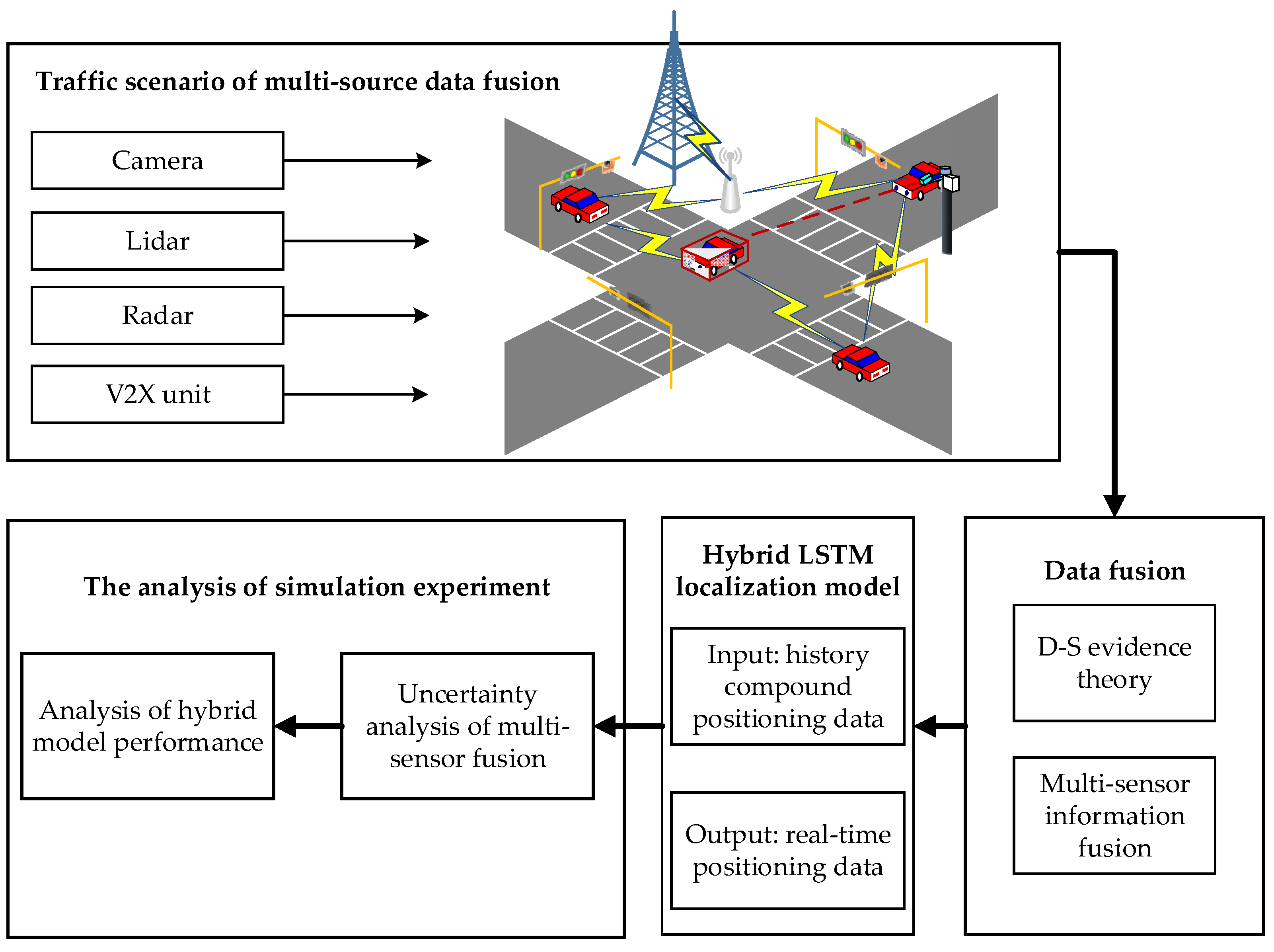
• Theoretical analysis and extensive experiment results, including the Dempster-Shafer (D-S) evidence theory-based multi-source data fusion method and hybrid neural networks, are provided to validate the proposed concept.

The remainder of this paper is organized as follows. The traffic scenario of multi-source data fusion is described in Section 2, where the vehicle-infrastructure information fusion method based on D-S evidence theory is constructed and clarified. Section 3 proposes the perception model of compound positioning information to improve the positioning accuracy of CEVs. Then, in Section 4, the training and test data are compared and analyzed to verify the proposed method. Finally, the conclusion is provided in Section 5. The technology roadmap of this paper is shown in Figure 1.

2. Multi-Source Data Fusion Based on D-S Evidence Theory

In order to integrate information from different sensors (e.g., on-board sensors, roadside sensors, etc.) and remove data redundancy, a method based on D-S evidence theory is proposed to solve the uncertainty of multi-sensor detection information, which can obtain vehicular compound positioning information. At the same time, traffic information data matrixes based on multi-source data fusion are constructed to improve the accuracy and reliability of the data.

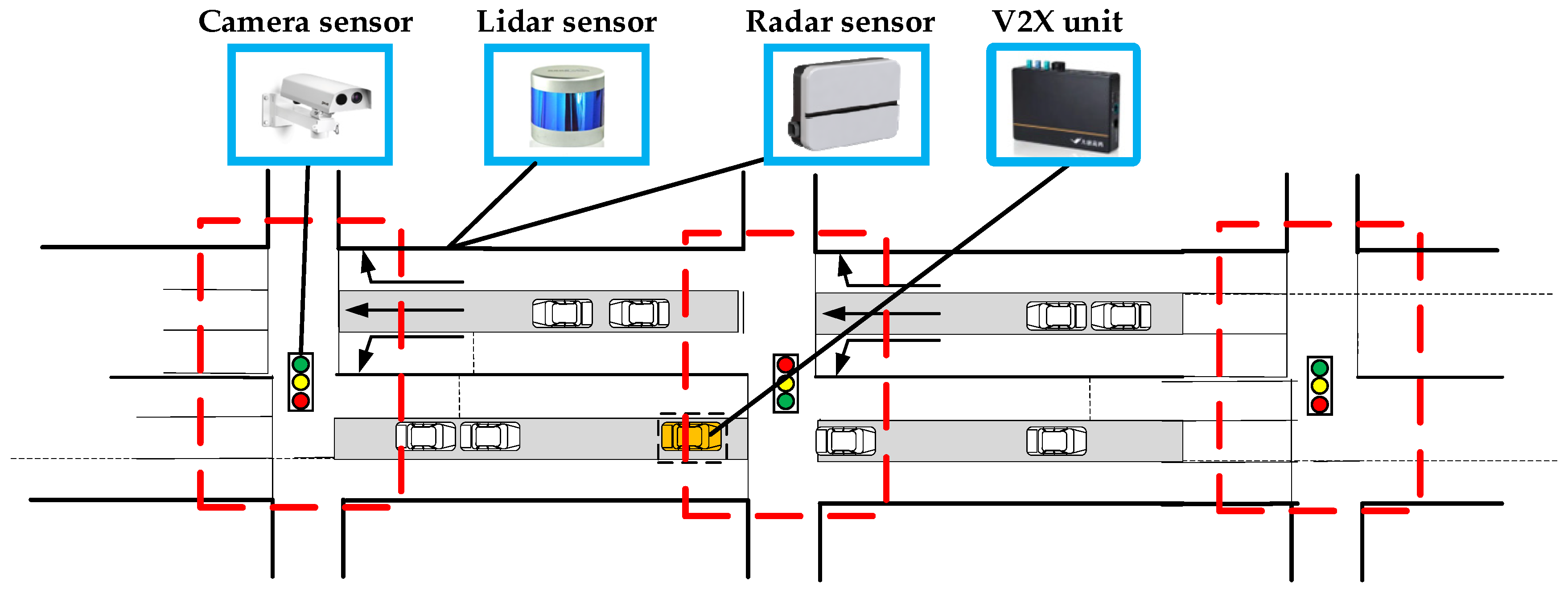
2.1. The Scenario of Multi-Source Data Fusion

Multi-source data in the scenario of vehicle-infrastructure can be obtained from roadside sensors and V2X units mounted on CEVs [38]. Roadside sensors include camera sensors, lidar sensors, and radar sensors.

The camera sensor is highly intuitive to provide a large amount of road information. Through the two-dimensional image features, the target vehicle can be better distinguished from other objects. Three-dimensional point cloud data can be output by lidar sensors, which have the advantages of a wide detection range and high detection accuracy. The 77 GHz radio waveforms can be emitted by the radar, with strong penetration and anti-interference ability, which can be applied in the detection of dynamic CEVs accurately in rainy and foggy weather. Different sensors use different communication methods to obtain traffic information for subsequent data fusion. Thereby, the vehicular positioning information can be obtained quickly and accurately. The fusion scenario is shown in Figure 2.

For multi-source data fusion, there are generally two types of data that need to be fused: the original data collected by each sensor and the detection information that has been reprocessed. According to the classification of abstraction level, data fusion can be divided into pixel level, feature level, and decision level [39]. The decision-level data fusion can still work when one or more sensors detect distortion, failure, and damage, thus ensuring the fault tolerance and real-time performance of the detection results. Therefore, this paper fuses the vehicular detection information. Through the fusion of multi-source data, the accuracy of vehicular compound positioning perception can be improved.

2.2. Data Fusion Rules of D-S Evidence Theory

The data collected by a single sensor have poor robustness, which usually lead to the uncertainty of detection results. The D-S evidence theory-based data fusion method can deal with uncertain, incomplete, and imprecise information. According to the characteristics of target detection, this paper assigns credibility assignments based on statistical evidence, which weights vehicular positioning information detected by different sensors. Then, credibility assignment of each sensor is obtained by a trust function, and the way of basic credibility assignment is shown in

Table 1. The basic credibility assignment.

	Sensor State	Detected (A)	Undetected (B)	Uncertain (C)
Sensor Type
Camera sensor (1)		m1 (A)	m1 (B)	m1 (C)
Lidar sensor (2)		m2 (A)	m2 (B)	m2 (C)
Radar sensor (3)		m3 (A)	m3 (B)	m3 (C)
V2X unit (4)		m4 (A)	m4 (B)	m4 (C)

. There are three detection states of the sensor, namely, detected vehicle, undetected vehicle, and uncertain detected vehicle, which can be represented by events A, B, and C, respectively.

The detection result of each sensor is considered as a piece of evidence. Then, the multi-sensor information is fused based on evidence fusion rules. Taking the fusion process of two sensors as an example, the calculation method is shown in Equation (1).

$$m_{1,2}(A)=\left(m_1\oplus m_2\right)(A)=\frac{1}{1-K}{\displaystyle \sum _{B\cap C-A\ne \varnothing }{m}_1}(B)m_2(C)$$

(1)

where K is the normalization coefficient. The calculation method is shown as follows:

$$K={\displaystyle \sum _{B\cap C=\varnothing }{m}_1}(B)m_2(C)$$

(2)

which can be equivalent to:

$$1-K={\displaystyle \sum _{B\cap C\ne \varnothing }{m}_1}(B)\cdot m_2(C)=1-{\displaystyle \sum _{B\cap C=\varnothing }{m}_1}(B)\cdot m_2(C)$$

(3)

Once the multi-sensor data are fused, the amount of evidence from each sensor will increase with the number of sensors. As a result, the data dimension grows geometrically, which reduces the efficiency of fusion. Therefore, the two pieces of evidence are fused based on the calculation in Equation (3), and the iterative process is continued until the fusion of multiple pieces of evidence is completed. The operation process is shown in Figure 3.

According to the D-S evidence theory, after fusing all sensor information, the maximum probability is regarded as the final decision, as shown in Equation (4). If Equation (4) is satisfied, then A is the final decision.

$$\{\begin{array}{l}m(A)-m(B)>{\epsilon }_1\hfill \\ m(\Theta )<{\epsilon }_2\hfill \\ m(A)>m(\Theta )\hfill \\ m(A)=\max \{m(A),m(B),m(\Theta )\}\hfill \end{array}$$

(4)

where ${\epsilon }_1$ and ${\epsilon }_2$ are the preset threshold.

If Equation (5) is satisfied, then B is the final decision:

$$\{\begin{array}{l}m(B)-m(A)>{\epsilon }_1\hfill \\ m(\Theta )<{\epsilon }_2\hfill \\ m(B)>m(\Theta )\hfill \\ m(B)=\max \{m(A),m(B),m(\Theta )\}\hfill \end{array}$$

(5)

In summary, the rules for the final decision are summarized as follows:

Rule 1: The trust value of the selected event detection result should be greater than that of other detection results, and the difference is greater than a certain lower limit.

Rule 2: The trust value occupied by uncertain events must be less than a certain upper limit.

Rule 3: The trust value of the selected event detection result must be greater than the uncertainty trust values.

Rule 4: The event with the largest trust value is selected as the detection result.

However, in the actual fusion process, the determination of thresholds ${\epsilon }_1$ and ${\epsilon }_2$ needs to consider the actual traffic fusion scenario, which can obtain better decision results by choosing different thresholds.

In the vehicular position judgment based on the probability fusion algorithm, the detection probabilities of four sensors are fused. Then, according to the fusion results, determine whether there is a vehicle at the position. According to the vehicular position detection results of each sensor, the detection results can be randomly combined in 16 combination forms, which is shown in

Table 2. The combination of the detection results for four sensors. “Yes” represents that a vehicle is detected at the position. “No” represents that there is no vehicle at the position.

	Combination Forms	1	2	3	4	5	6	7	8	9	10	11	12	13	14	15	16
Sensors
Camera		Yes	Yes	Yes	Yes	No	Yes	Yes	No	Yes	No	No	No	No	No	No	No
Lidar		Yes	Yes	Yes	No	Yes	Yes	No	No	No	Yes	Yes	Yes	Yes	No	No	No
Radar		Yes	Yes	No	Yes	Yes	No	No	Yes	Yes	No	Yes	No	No	Yes	No	No
V2X unit		Yes	No	Yes	Yes	Yes	No	Yes	Yes	No	Yes	No	Yes	No	No	Yes	No

.

Taking composition form 1 as an example, the camera, lidar, radar, and V2X unit simultaneously detect the presence of vehicles in the detected area. The basic reliability of four sensors are $m_1=(A,B,\Theta )$, $m_2=(A,B,\Theta )$, $m_3=(A,B,\Theta )$, $m_4=(A,B,\Theta )$, respectively. The multi-source data fusion process under this combined form is shown as follows:

• For $m_{1\oplus 2}$ fusion, the normalized coefficient 1-K value is obtained using the D-S evidence fusion rule, which is shown in Equation (6).

$$1-K=m_1(A)\cdot m_2(A)+m_1(A)\cdot m_2(\Theta )+m_1(\Theta )\cdot m_2(A)$$

(6)

where K is the degree of evidence conflict.

• The values of the mass function for each hypothesis are obtained as follows:

$$\begin{array}{l}{m}_1(A)\oplus m_2(A)=\frac{1}{1-K}\cdot (m_1(A)\cdot m_2(A)+m_1(A)\cdot m_2(\Theta ))+m_1(\Theta )\cdot m_2(A)))\\ m_1(B)\oplus m_2(B)=\frac{1}{1-K}\cdot (m_1(A)\cdot m_2(B)+m_1(B)\cdot m_2(\Theta ))+m_1(\Theta )\cdot m_2(B)))\end{array}$$

(7)

• The confidence intervals are obtained as follows:

The confidence interval of A is $[m_1(A)\oplus m_2(A),m_1(A)\oplus m_2(A)+m_1(\Theta )\cdot m_2(\Theta )]$. The confidence interval of B is $[m_1(B)\oplus m_2(B),m_1(B)\oplus m_2(B)+m_1(\Theta )\cdot m_2(\Theta )]$. The length of the confidence interval is $m(\Theta )$.

• Therefore, the credibility of $m_{1\oplus 2}$ fusion is $m_{1\oplus 2}=\left[\begin{array}{l}m\left(A_1\right)\hfill \\ m\left(A_2\right)\hfill \\ m(\Theta )\hfill \end{array}\right]$
• According to D-S evidence theory, $m_{1\oplus 2}$ and $m_3$ are fused, which represent the combined credibility of camera, lidar, and radar is obtained: $m_{1\oplus 2\oplus 3}$.
• In the same way, the credibility of four sensors fusion is finally obtained, which is $m_{1\oplus 2\oplus 3\oplus 4}$.

Table 3. Fusion results of 16 combination forms.

Combination Form	Sensor Number	m(A)	m(B)	m(Θ)	Fusion Result
1	4	0.949350	0.050634	0.000016	A
2	3	0.777015	0.222413	0.000572	A
3	3	0.798684	0.200929	0.00387	A
4	2	0.419643	0.571429	0.008929	B
5	3	0.981207	0.018715	0.000078	A
6	2	0.906375	0.090504	0.003121	A
7	2	0.901087	0.098755	0.00159	A
8	1	0.65	0.28	0.07	A
9	3	0.901087	0.098755	0.000159	A
10	2	0.627191	0.36803	0.00478	A
11	2	0.657519	0.339188	0.003293	A
12	1	0.22	0.72	0.06	B
13	2	0.962065	0.037144	0.00079	A
14	1	0.82	0.15	0.03	A
15	1	0.84	0.14	0.02	A
16	0	——	——	——	Θ

shows the credibility comparison results of 16 combination forms.

Compared with the fusion results of 16 combination forms, it can be observed that the uncertainty of fusion results decreases with more sensors. It is proved that the false rate of detection results is lower after the fusion of multi-sensor detection information by D-S evidence theory.

3. The Perception Model of Compound Positioning Information

In Section 2.2, D-S evidence theory is used to fuse the multi-sensor detection information collected by four detectors, so that the vehicular position probability with high accuracy can be obtained. This paper proposes a hybrid neural network model based on the LSTM framework, which can obtain the compound positioning information of the CEV in real time. The structure of the hybrid LSTM model is shown in Figure 4.

As shown in Figure 4, the latitude, longitude, and time of CEV position information are taken as the inputs of the hybrid LSTM model, where L = {P₁, P₂,…, P_n} denotes the set of track points of the CEV within n time steps, P_i = (lat_i, lon_i, t_i) denotes the i-th positioning point of CEV, lat_i denotes the latitude, lon_i denotes the longitude, and t_i denotes the time. These inputs are passed through the data preprocessing layer, CNN layer, LSTM layer, self-attention layer, dropout layer, and dense layers. The final output of the model is vehicular compound positioning information (lat_i, lon_i, t_i) in real time.

After the input data are extracted, the input data will be transmitted to the LSTM layer, and the historical data are stored and transmitted downward along the positioning sequence to predict the next position. The attention vector is calculated through the previous hidden state from the LSTM layer to the self-attention layer. At the same time, the dropout layer can prevent the overfitting of the neural network, and the fully connected layer mainly classifies the feature vector. Finally, the output layer combines the output of the previous layer to obtain the CEV compound positioning data in real time.

In fact, the calculation of compound positioning P’ perception is to learn the mapping function f, which is based on intersection topology matrix N and positioning vector P, as shown in Equation (8):

$${P^{\prime }}_t=f(N;(P_{t-n},\dots ,P_{t-1},P_t))$$

(8)

where n denotes length of historical time series.

3.1. Date Preprocessing Layer

In the scenario of vehicle-infrastructure information fusion, each sensor is an independent information source. Therefore, the position coordinates of the CEV collected by each sensor can be assigned as the basic probability of evidence, and these pieces of evidence do not completely conflict.

Therefore, in the preprocessing layer, multiple trust functions can be synthesized into a trust function by the corresponding evidence synthesis rules, and this trust function can be seen as the comprehensive trust function of these pieces of evidence. Moreover, the basic probability assignment of four sensors is used to fuse the multi-sensor positioning data to obtain the comprehensive trust estimation of each reference point. Finally, through the D-S evidence synthesis rule, the comprehensive trust estimates m(A) and m(B) of two definite states and an uncertain state trust estimate m(C) are obtained. Similarly, the comprehensive trust estimation of the state relationship between the target and multiple reference points can be calculated.

According to the relationship between trust function and likelihood function, an ideal reference point should be satisfied by the following requirement: the credibility of the target at the reference point is greater than the credibility of the target not at the reference point, and greater than the uncertainty of the target, as shown in Equation (9):

$$\begin{array}{l}{m}_i(A)>m_i(B)\\ m_i(A)>m_i(C)\end{array}$$

(9)

According to Equation (9), the reference point set of vehicular position can be obtained, and these reference points continue to be used as inputs to the next layer.

3.2. CNN Layer

A convolutional neural network (CNN) is used to process data with multiple array forms. Considering the characteristics of CEV tracking points, the two-dimensional data array of position and time is adopted in this paper. The combination of position and time variables at each tracking point of the CEV are extracted by the CNN to capture correlation between variables.

The CNN has a unique network structure, which consists of five layers: input layer, convolution layer, pooling layer, fully connected layer, and output layer. The structure of CNN is shown in Figure 5.

• Input layer

The input layer is used to capture the spatial features information of road traffic. In this paper, the traffic spatial features within the intersection range are transformed into the pixel matrix as the input of the model. As shown in the input layer in Figure 5, the traffic feature of the intersection area can be regarded as a pixel matrix, whose matrix dimension can be expressed by [length × width × depth], where length and width represent image size, and depth represents the color channel.

2.

Convolution layer

The convolution layer is the core layer of the CNN, which extracts the spatial features of traffic parameters using a convolution algorithm. The filter or convolution kernel is mainly used for feature extraction of the input spatial matrix. The convolution operation of the CNN can be expressed as Equation (10).

$$a_{i,j}=f\left({\displaystyle \sum }_{m=0}^{M-1}{\displaystyle \sum }_{n=0}^{N-1}{w}_{m,n}{x}_{i+m,j+n}+w_b\right)$$

(10)

where the size of the filter matrix is M rows and N columns; x_i,j represents the input two-dimensional data at i-th row and j-th column; w_m,n represents weight value at m-th row and n-th column of the filter matrix; w_b represents the filter bias value; f is the activation function; a_i,j represents the i-th row and j-th column of the feature map.

3.

Pooling layer

The pooling layer can reduce the number of nodes in the fully connected layer, to reduce the parameters in the whole neural network. Although the pooling layer will not change the depth of the matrix, it can reduce the size of the matrix. The pooling layer can retain effective information by reducing feature dimensions of data. Generally, pooling methods include maximum pooling, mean pooling, and mixed pooling.

4.

Fully connected layer and output layer

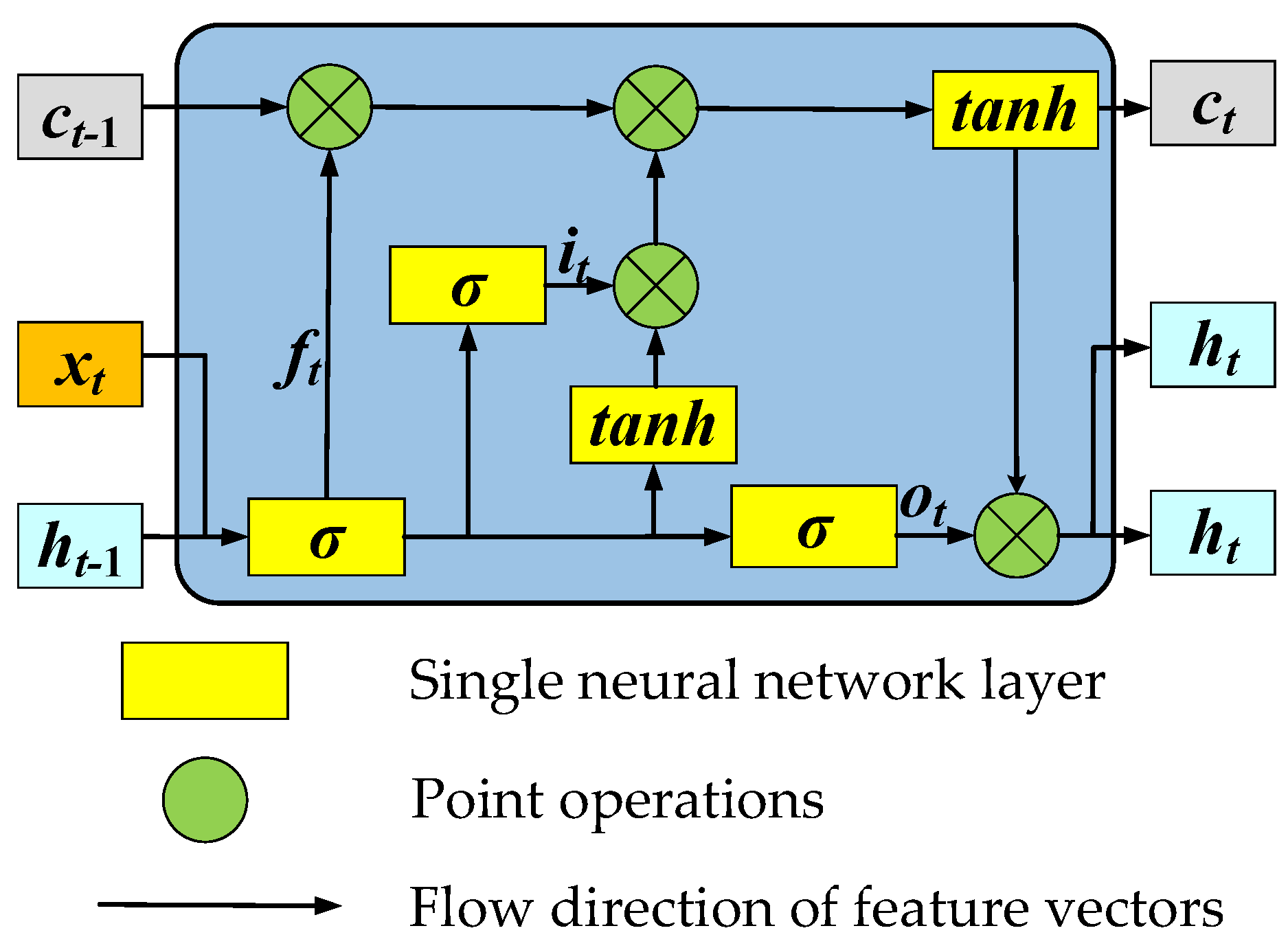
After several rounds of convolution and pooling, the feature matrix of the vehicular track state at the intersection has been abstracted into features with higher information content. Lastly, the output dimension is adjusted by the fully connected layer and the output layer, and the final result is output at the same time.

3.3. LSTM Layer

In terms of time dimension, the LSTM network with deep structure has memory units that store historical time series information, which can generate multi-step predictive variables through mass training by supervised learning. The LSTM network can automatically extract and transmit the relevant information along the long sequence chain for prediction, which is suitable for learning the sequential motion pattern of CEV positioning data. Therefore, the LSTM network is selected to obtain the compound positioning information of the CEV in real time.

The LSTM network is a kind of recurrent neural network in time series, which can remember information within a certain time. The LSTM network has three gates, including the input gate, forget gate, and output gate. The structure of the LSTM neural network is shown in Figure 6.

At time t, there are three inputs in the LSTM network: the vehicular compound positioning data x_t, and the output value h_t−1 and c_t−1 in the previous hidden layer. The output of the LSTM network is the real-time compound positioning data of the CEV. The status of the input gate, forget gate, and output gate in the LSTM network are i_t, f_t, and o_t, which are from 0 to 1. The calculation process can be summarized as follows:

$$f_t=\sigma (W_{xf}{x}_t+W_{hf}{h}_{t-1}+b_f)$$

(11)

$$i_t=\sigma (W_{xi}{x}_t+W_{hi}{h}_{t-1}+b_i)$$

(12)

$$o_t=\sigma (W_{xo}{x}_t+W_{ho}{h}_{t-1}+b_o)$$

(13)

$$c_t=f_t{c}_{t-1}+i_t\tanh (W_{xc}{x}_t+W_{hc}{h}_{t-1}+b_c)$$

(14)

$$h_t=o_t\tanh (c_t^{})$$

(15)

where $W_{xf}$, $W_{xi}$, $W_{xo}$, $W_{xc}$ represent the weight matrices for the spatial feature; input x_t is the compound positioning data; $W_{hf}$,$W_{hi}$,$W_{ho}$,$W_{hc}$ represent the weight matrices of hidden layer $h_t$ respectively; $b_f$, $b_i$, $b_o$, $b_c$ represent the bias vector, respectively; $\sigma$ and tanh represent the sigmoid function and hyperbolic tangent function, which are defined in Equations (16) and (17).

$$\sigma (x)=\frac{1}{1-e^{-x}}$$

(16)

$$\tanh (x)=\frac{2}{1+e^{-x}}-1$$

(17)

In addition, the training process of the LSTM network can continue if the input value is too large or even empty. Therefore, even if the error of the fused positioning input value is too large or even empty, the training of the model can be carried out.

3.4. Self-Attention Layer

In the self-attention mechanism layer, the correlation between different positions in the CEV trajectory and the feature information of input position in the previous layer in each step of the training process can be paid more attention by the hybrid model. The self-attention mechanism can enhance the performance of the hybrid LSTM model and improve the compound positioning accuracy. The calculation process is shown as follows:

$$g_{t,t^{\prime }}=\tanh \left(W_g{h}_t+W_{g^{\prime }}{h}_{t^{\prime }}+b_g\right)$$

(18)

$$e_{t,t^{\prime }}=\sigma \left(W_a{g}_{t,t^{\prime }}+b_a\right)$$

(19)

$$a_{t,t^{\prime }}=\frac{\exp \left(e_{t,t^{\prime }}\right)}{{{\displaystyle \sum }}_j\exp \left(e_{t,j}\right)}$$

(20)

$$A_t={\displaystyle \sum }_{t^{\prime }}{a}_{t,t^{\prime }}{h}_{t^{\prime }}$$

(21)

where h_t and h_t’ represent the hidden state of the LSTM layer in current time step t and the previous time step t′, respectively; $\sigma$ represents the sigmoid function; W_g and W_g′ represent the weight matrices corresponding to h_t and h_t’; W_a represents the weight matrix corresponding to its nonlinear combination; b_g and b_a represent deviation vectors.

The attention output A_t at the time step t is the weighted sum of all previously hidden states h_t’, which is weighted by a_t,t′. Additionally, a_t,t′ represents the similarity or dependence between h_t and h_t′, where the similarity is the relationship between the current position at time t and the previous position at t’ in the input trajectory.

3.5. Dropout Layer

The dropout layer refers to the discarding of neural network elements according to certain probabilities during training of deep learning networks. However, in model training, problems such as overfitting and time-consuming issues are always encountered. Therefore, the dropout function is mainly to reduce the occurrence of overfitting during the experiment. The dropout layer can improve the robustness of the model when training the vehicular trajectory data and improve the model’s generalization ability.

To sum up, the hybrid neural network model based on the CNN and LSTM is proposed in this paper. Firstly, the original CEV position data are preprocessed to ensure the stability of positioning sequence data. Convolutional networks are used to capture the depth features of data in the model. Then, the position sequence with depth characteristics is input into the LSTM layer, and the time features are obtained by multi-step prediction variables. Finally, the self-attention mechanism is combined with the LSTM network to obtain the position correlation in the CEV positioning data series. Therefore, the hybrid LSTM model can better capture the position dependence of each compound positioning trajectory sequence and improve the positioning effect of the hybrid LSTM model in the self-attention layer.

4. Field Experiment and Analysis

In order to verify the proposed hybrid model in this paper, a typical urban intersection was selected as the experiment scenario [40,41]. In this experiment, real-time vehicular compound positioning data were selected as the model input.

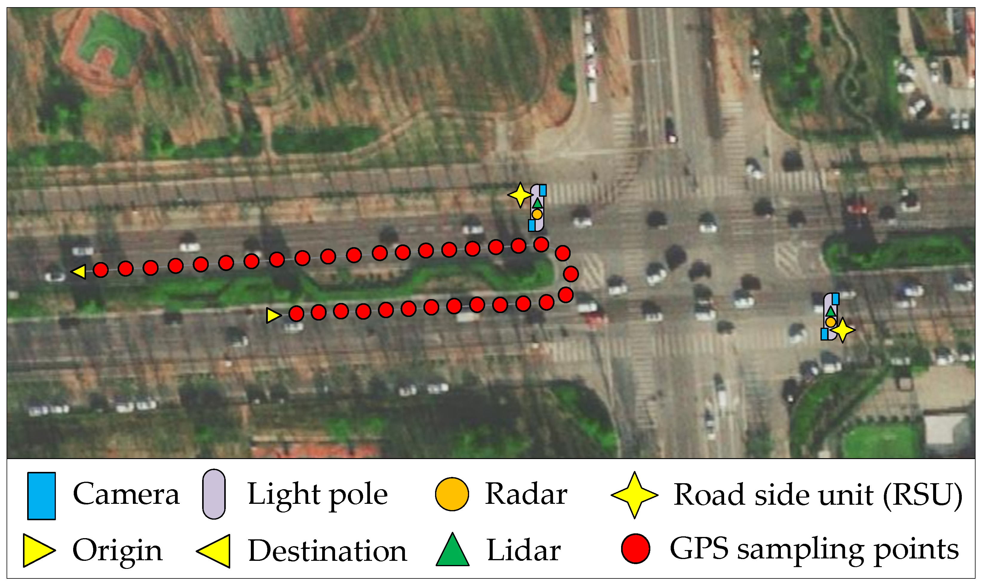
4.1. Test Field and Datasets

In the experiment, an intersection in Shijingshan District, Beijing was selected as the test field for trajectory information collection of the CEVs. There are four lanes at the entrance of the intersection, with a U-turn lane as the left-most lane.

There were three CEVs in this experiment, named C₁, C₂, and C₃, respectively. In addition, CEVs were within the detection range of roadside sensors during the whole driving process. In Figure 7, the origin and destination of the driving route are marked. The CEV first passes through the straight road section at a uniform speed from the left-most lane, then makes a U-turn at the intersection, and finally runs at a uniform speed.

Roadside multi-source sensors include camera, lidar, and radar sensors, which can not only track the position of the target vehicle in real time, but also detect the environmental parameters of roadside infrastructure. The V2X unit mounted on the CEVs can obtain positioning information based on positioning data from CAN-Bus. In the field test, we also calculated the actual traffic flow of the road at different times based on the roadside multi-source sensors.

About 12,000 pieces of effective data were obtained after preprocessing, cleaning, and merging the data collected in the experiment, as shown in

Table 4. Dataset example.

ID	V2X	Longitude	Latitude	Steering Angle (°)	Speed (m/s)	Acceleration (m/s2)	Horizontal Distance (m)	Heading Angle (°)
76	Yes	116.2138743	39.9306605	2.3	0.16	−0.16	7.82	88.22
77	No	116.2139375	39.9306708	——	2.11	——	12.14	82.92
⋮	⋮	⋮	⋮	⋮	⋮	⋮	⋮	⋮
95	No	116.2127606	39.9306348	——	2.14	0.20	17.17	154.52
96	No	116.2120122	39.9306519	——	5.58	——	15.17	82.59

.

In order to improve the effect of model training, we divided the collected data into a test set and training set, in which 80% of the data were randomly selected as the training data set and the other 20% as the test data set.

4.2. Parameter Setting and Evaluation Index

The construction of the hybrid model proposed in this paper was based on the NVIDIA Geforce GTX 1050ti GPU hardware platform. Moreover, the hybrid network was trained with the PyTorch 1.4 framework. Considering the range of features and the computing power of the device, a 16 × 16 convolution layer was selected in the CNN. Meanwhile, in order to preserve the features to be detected as completely as possible, we chose the size of the pooling layer as 8 × 8. The number of hidden layers in the LSTM was related to the prediction error and complexity of the model. Through practical verification, the number of hidden layers was set to 2, and there was no overfitting. Moreover, the number of nodes in the hidden layer needs to match the number of hidden layers, so we set the number of nodes in the hidden layer to 200. The hybrid network model has been trained and adjusted, and the main parameters of each layer network model are shown in

Table 5. Parameter setting of hybrid LSTM model.

Parameters		Value
CNN	Input layer size	256 × 256
	Convolution layer size	16 × 16
	Pooling layer size	8 × 8
LSTM	Number of hidden layers	2
	Number of hidden layer nodes	200
	Epoch	20
	Batch Size	100
	Loss Function	MSE
	Learning Rate	0.001
	Optimizer	Adam

.

After inputting the vehicular positioning sequence into the model and obtaining the corresponding output, it was necessary to compare the output of the model with the label used for supervision training. Since the outputs of the neural network were two-dimensional coordinates, the model selects the minimum mean square error (MSE) as the loss function to evaluate the positioning results, as shown in Equation (22). The smaller the MSE is, the better the fitting of the neural network, and the training set is shown as follows:

$$MSE=\frac{1}{n}{{\displaystyle \sum _1^n(outpu{t}_i-labe{l}_i)}}^2$$

(22)

where output_i is the output of the network; label_i is the label of supervised training.

In order to make a clearer and intuitive evaluation of the model fitting results, root mean square error (RMSE) and mean absolute percentage error (MAPE) are given as one of the evaluation indexes of fusion performance. The smaller the RMSE, the better the compound positioning effect. The specific RMSE and MAPE definitions are shown in Equations (23) and (24).

$$RMSE=\sqrt{\frac{1}{m}{\displaystyle \sum }_{i=1}^m{\left(\widehat{y_i}-y_i\right)}^2}$$

(23)

$$MAPE=\frac{100\%}{n}{\displaystyle \sum }_{i=1}^n\left|\frac{{\widehat{y}}_i-y_i}{y_i}\right|$$

(24)

where ${\widehat{y}}_i$ represents the output of the network compound positioning; $y_i$ represents the actual position of the vehicle; n and m are the number of samples calculated by RMSE and MAPE, respectively.

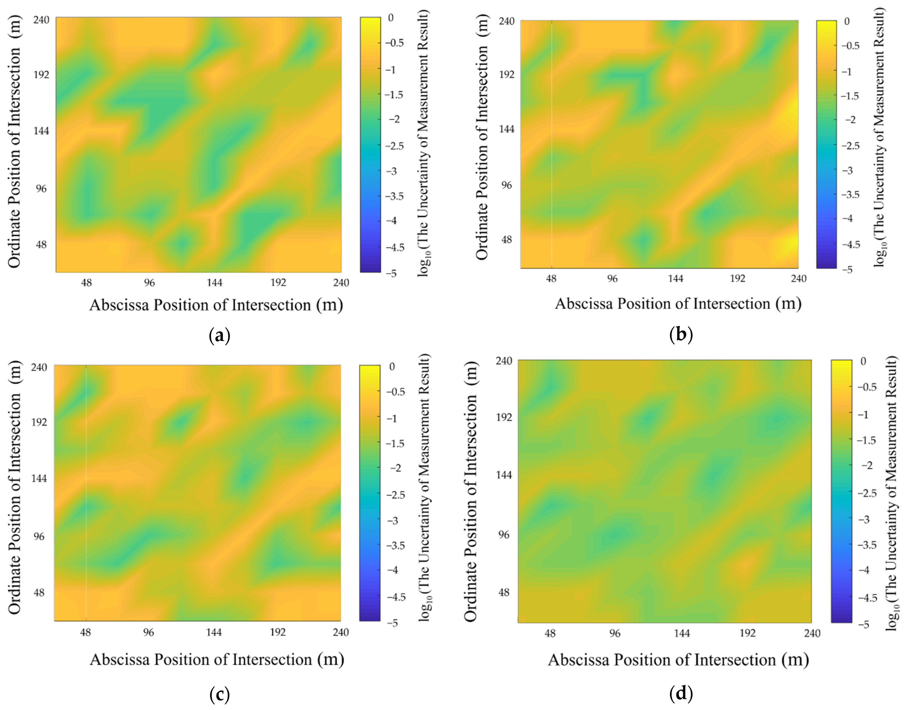
4.3. Uncertainty Analysis of Multi-Source Data Fusion

Before multi-sensor fusion, the detection effect of each single sensor was tested after sensor perception correction, whose detection errors are shown in

Table 6. Comparison results of detection error.

	Sensor Category	Camera	Lidar	Radar	V2X Unit
Error
Maximum (m)		18.4623	0.8268	2.0168	20.9980
Minimum (m)		0.1917	0.0082	0.0607	0.0488
Average (m)		3.5881	0.2111	0.7138	8.1386
MAPE		19.26%	0.70%	23.72%	26.87%

. Comparing the measured value with the collected data, the maximum value (m), minimum value (m), and average value (m) of the detection error of each single sensor are listed in Table 6, and the MAPE is also calculated and listed in Table 6.

In order to better evaluate the effect of multi-source data fusion, the uncertainty should be analyzed firstly. As shown in Section 2.2, in order to reduce the uncertainty of target detection by a single sensor, this paper selects multi-sensors to fuse information without changing the contradiction degree to increase the information amount.

Based on the distribution of uncertainty after statistical data fusion, the detection results of uncertainty distribution for each sensor are shown in Figure 8. The detection result of uncertainty distribution after multi-source data fusion is shown in Figure 9.

By comparing Figure 8 and Figure 9, the uncertainty of the fused data is significantly lower than that before the data fusion operation in the detection area. The average value of uncertainty decreased from 8% to 0.03%, which is about 0.38% of the original level. The reduction of uncertainty indicates that the accuracy of data recognition is higher, and the corresponding detection error is smaller after data fusion.

The uncertainty of some regions with high uncertainty in Figure 8 is also significantly reduced in Figure 9 after multi-source data fusion. For example, in areas with high vehicle density, the vehicle speed is unstable, which leads to low detection accuracy of individual sensors and high uncertainty in the evaluation of this region. Therefore, by comparing the distribution of uncertainty, it can be seen that the detection results based on multi-source data fusion have higher reliability.

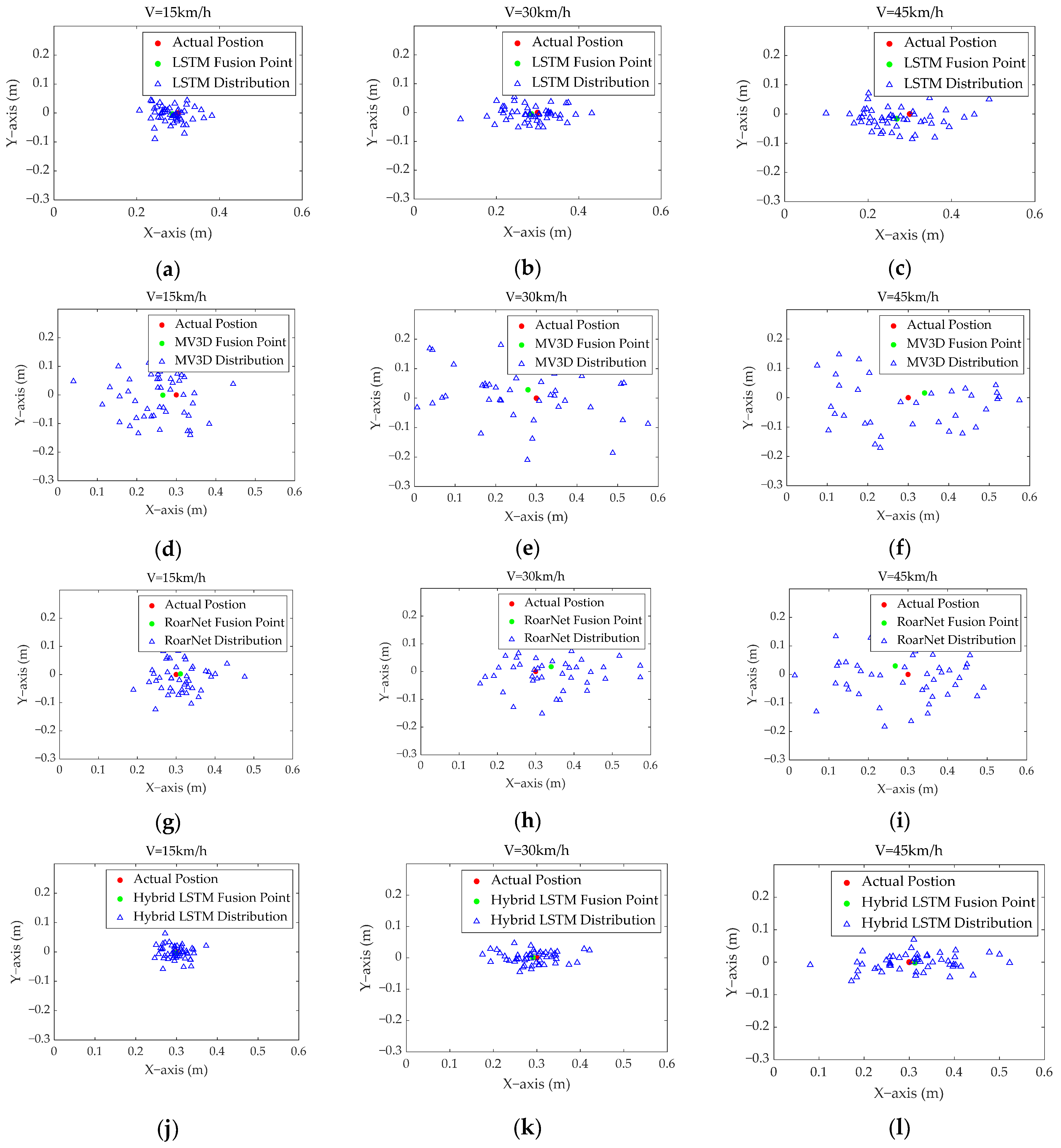
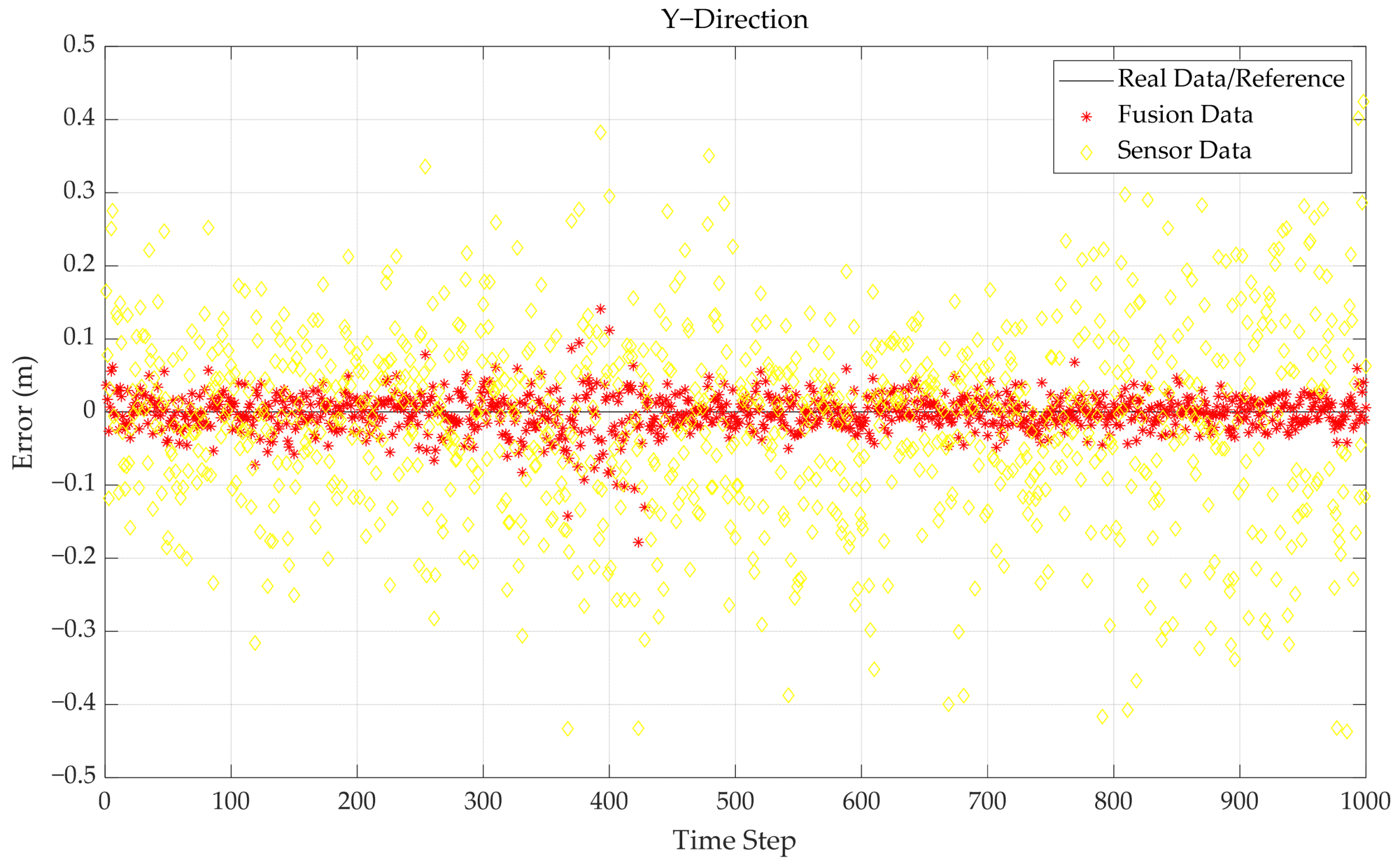
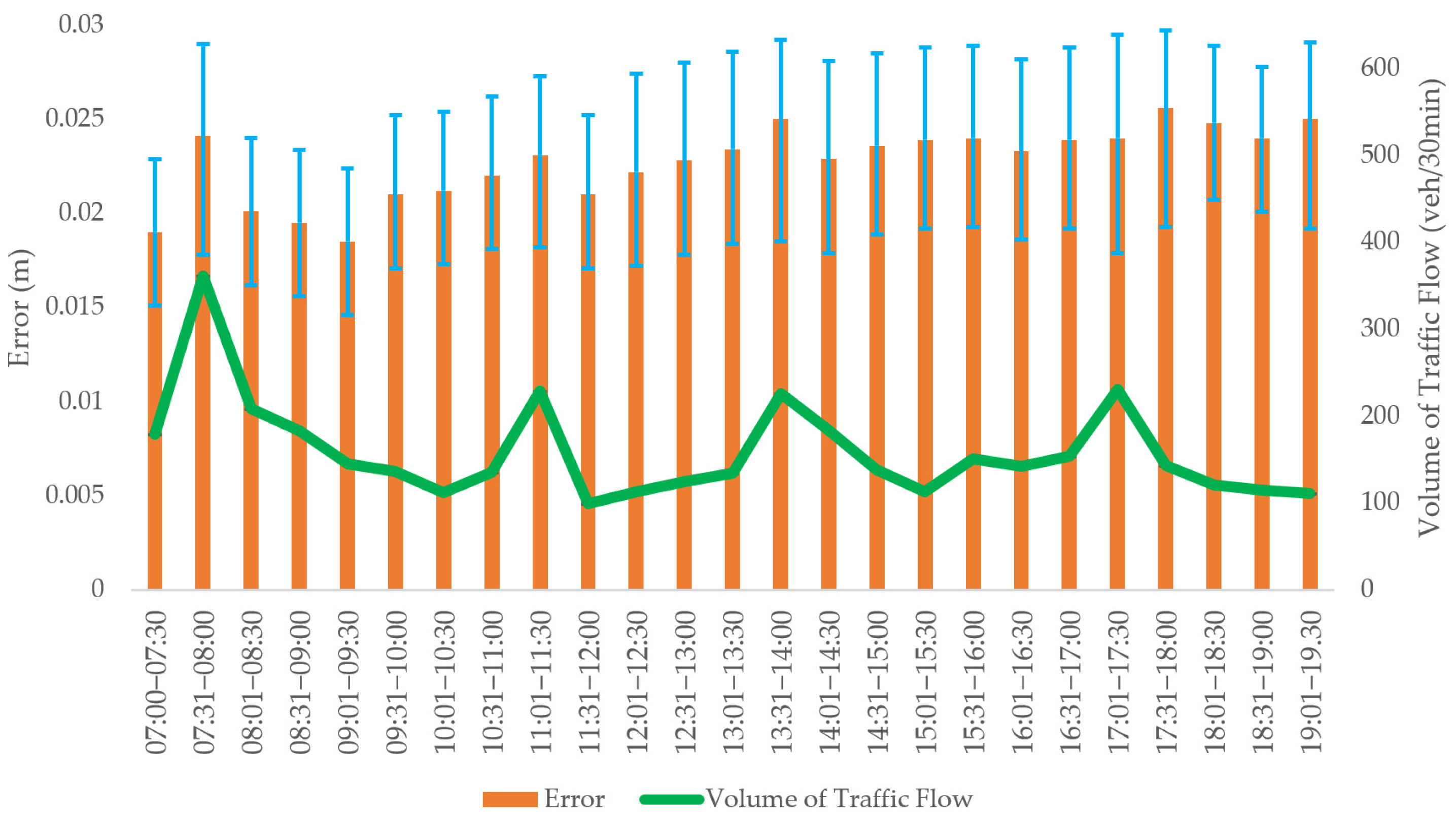
4.4. Analysis of Compound Positioning Model

In the process of model training, the RMSE of the hybrid LSTM model changes with increase of the number of iterations, as shown in Figure 10. In order to present the trend of RMSE function more intuitively, Figure 10 shows the smoothed RMSE curve and the original RMSE curve, respectively. The smoothed RMSE curve uses the method of a 5-point moving average to smooth the original data. Moreover, the RMSE value of the hybrid LSTM model tends to be stable after 200 rounds of iterations. Owing to the LSTM needs of the use of the historical sequence to predict the output, the training RMSE value in the initial iteration is high.

In order to evaluate the performance of the hybrid LSTM model in compound positioning perception, the LSTM model was compared in the comparative experiment [42]. At the same time, some network structures still have certain advantages in dealing with the field of compound positioning. Considering that a multi-view 3D object (MV3D) has the characteristics of less resource occupation and RoarNet has the characteristics of high robustness and high accuracy, MV3D and RoarNet were selected as comparative models in the experiment [43,44]. In the experiment, the calculation times of LSTM, MV3D, RoarNet, and hybrid LSTM models were 122, 45, 87, and 48 ms, respectively. Since the collection period of sensors was 50 ms, the total calculation periods of these models were 122, 50, 87, and 50 ms, respectively.

The comparative experiment randomly selects anchor points and randomly positioned each anchor point 50 times under different speed conditions, to verify the compound positioning effect of different models. The compound positioning solution results of the four methods were recorded, and the distribution is shown in Figure 11.

In the comparative experiment at different speeds, the positioning status of the MV3D and RoarNet model was relatively discrete and the positioning accuracy was low, which is shown in Figure 11. In addition, as the vehicular speed was below 30 km/h, the compound positioning distribution of the LSTM is similar to the method based on the hybrid LSTM model. However, once the speed increases, the stability of the LSTM model was affected, and the results of compound positioning were more divergent, which cannot describe the positioning information of the CEV accurately. Therefore, it can be seen from the distribution map that the distribution region of the compound positioning was more concentrated, and the distribution shape was more convergent after training of the hybrid LSTM model. For compound positioning results with a large offset, they are closer to real values after correction by the hybrid LSTM model.

In order to verify the reliability of the hybrid LSTM model, the test numbers of anchor points were increased in the same experimental scenario.

Table 7. Average difference between real and trained position of the four models (m).

Model	Anchor 2	Anchor 3	Anchor 4
LSTM	0.1179	0.0821	0.0630
MV3D	0.1475	0.1322	0.1071
RoarNet	0.1121	0.0690	0.0610
Hybrid LSTM	0.0910	0.0609	0.0399

shows the average difference between the trained position of the four models and the real position when the three additional anchors (Anchor 2, Anchor 3, and Anchor 4) were involved in compound positioning.

In Table 7, with the increase of anchors, the average difference between the trained position of models and real position gradually decreases. Especially for the hybrid LSTM model, when four anchors participate in positioning at the same time, the average difference is only 0.0399 m, which can satisfy most vehicle requirements of positioning accuracy. Therefore, the above experimental results show that, compared with the LSTM, MV3D, and RoarNet models, the hybrid LSTM model can effectively achieve real-time vehicular compound positioning based on multi-source sensor fusion data, under the limited resource conditions.

In order to evaluate the perception accuracy of the hybrid LSTM model, the training effects of the model before and after multi-source data fusion were compared. The positioning effect of CEVs collected by single sensors and multi-source data fusion is shown in Figure 12.

As shown in Figure 12, the effect of single sensor positioning is worse than that of multi-source data fusion positioning. In the same time series, the vehicular positioning data after fusion processing is closer to the real data, where the positioning accuracy is 0.0905 m. Based on the compound positioning model, the fused data not only performs well in the accuracy of data, but also performs well in the stability of data fluctuation.

In addition, the errors in different time steps for the X and Y direction were analyzed, which is shown in Figure 13 and Figure 14. The black straight line is the reference standard value of tested CEV; the red stars are the data errors of the fused data in different time steps for the X or Y direction; and the yellow circles are the optimal sensor errors of the current single sensors in different time steps for the X or Y direction.

According to the trajectories of the CEV in Figure 12, it can be observed that the CEV decelerates when the time step is 0 (error convergence for the X direction); completes the U-turn in the period of about 300–500 time steps (error transformation for the X and Y direction); then, the vehicle accelerates away from the sensing area (error divergence for the X direction). After analysis, the following conclusions can be drawn: Firstly, the error of the fused data is significantly more convergent than that of the vehicle single sensor. Secondly, the error of the vehicle in the forward direction is significantly smaller than that in the vertical direction. Thirdly, the error of the vehicle in the forward direction is positively correlated with vehicular speed. In addition, more than 97.9% of the detection data are less than 0.1 m, which meets the accuracy requirements of high-precision perception.

The above models were trained on the dataset respectively, and the error values of RMSE and MAE were used as evaluation indexes to compare the training performance of each model. The comparison results are shown in Figure 15.

It can be seen from Figure 15 that the hybrid LSTM model is the smallest error in the perception of target position. It is proven that the hybrid LSTM model has obvious advantages in compound positioning of CEVs based on multi-source data fusion.

In different periods of time, three CEVs were tested in an intersection to verify the detection effect of CEVs’ compound positioning under different traffic flows. The analysis of vehicular detection error at different traffic flows and time periods is shown in Figure 16.

In Figure 16, the green polyline represents the average volume of traffic flow in the current period, and the orange bars represent the average error of the tested CEV during this period, where the upper edge and the lower edge represent the maximum and minimum error detection of a CEV in the driving cycle. Analysis of the situation shown in Figure 16 has shown that there is a certain positive correlation between the vehicle detection error and the volume of traffic flow, while the detection time has no direct correlation with detection error. The reason for the decrease of detection accuracy may be due to the increased probability of vehicles being blocked in high-saturated traffic flow. However, the maximum detection error occurs in the morning peak hours, which is still lower than 0.03 to meet the high-precision positioning requirements of CEVs.

5. Conclusions

This paper mainly studies the vehicular compound positioning of CEVs based on multi-source data fusion technology in a vehicle-infrastructure information perception environment. First, the development of the existing real-time compound positioning method and vehicle communication method were analyzed. Secondly, a deep learning-based vehicle-infrastructure information fusion method was proposed to perceive the real-time driving position of CEVs. Then, this paper conducted an actual vehicle test by designing a traffic perception scenario based on vehicle-infrastructure information fusion. Finally, by analyzing and sorting out the real vehicle data, it was proven that the model proposed in this paper can accurately and efficiently complete the real-time positioning of CEVs.

In addition, there are still limitations in the research of this paper, which need to be further improved in follow-up work. In our study, the influence of objective conditions was not considered; for example, communication delay and data packet loss on the compound positioning accuracy of CEVs.

In future research, we will further improve the traffic scenarios, and consider the problems of data packet loss and communication delay during data transmission. Furthermore, there are many driving behaviors in the driving process of CEVs, such as continuous turning, linear acceleration and deceleration, sharp U-turns, etc., which depend on high-precision compound positioning. Therefore, how to guide the CEVs to make decisions based on the compound positioning information is also the direction of future research. Therefore, how to improve the intelligent driving decision-making and control ability of CEVs based on compound positioning information is also a direction of future research.

References

1. Scamarcio, A.; Metzler, M.; Gruber, P.; De Pinto, S.; Sorniotti, A. Comparison of anti-jerk controllers for electric vehicles with on-board motors. IEEE Trans. Veh. Technol. 2020, 69, 10681–10699. [Google Scholar] [CrossRef]
2. Aiman, M.A.; Mohammed, N.A. Comparison of the overall energy efficiency for internal combustion engine vehicles and electric vehicles. Environ. Clim. Technol. 2020, 24, 669–680. [Google Scholar] [CrossRef]
3. Machado, F.A.; Kollmeyer, P.J.; Barroso, D.G.; Emadi, A. Multi-speed gearboxes for battery electric vehicles: Current status and future trends. IEEE Trans. Veh. Technol. 2021, 2, 419–435. [Google Scholar] [CrossRef]
4. Li, X.; Wang, Y.G.; Cui, H.J.; Zhu, M.Q.; Wang, X.T. Stability analysis of complex heterogeneous traffic flow under connected and autonomous environment. J. Transp. Syst. Eng. Inf. Technol. 2020, 20, 114–120. [Google Scholar] [CrossRef]
5. An, Q.; Shen, Y. On the information coupling and propagation of visual 3d perception in vehicular networks with position uncertainty. IEEE Trans. Veh. Technol. 2021, 70, 13325–13339. [Google Scholar] [CrossRef]
6. Bolufe, S.; Cesar, A.M.; Sandra, C.; Samuel, M.S.; Demo, R.; Evelio, M.G.F. POSaCC: Position-accuracy based adaptive beaconing algorithm for cooperative vehicular safety systems. IEEE Access 2020, 8, 15484–15501. [Google Scholar] [CrossRef]
7. Wang, P.W.; Liu, X.; Wang, Y.F.; Wang, T.R.; Zhang, J. Short-term traffic state prediction based on mobile edge computing in V2X communication. Appl. Sci. 2021, 11, 11530. [Google Scholar] [CrossRef]
8. Hossain, M.A.; Elshafiey, I.; Al-Sanie, A. Cooperative vehicle positioning with multi-sensor data fusion and vehicular communications. Wirel. Net. 2019, 25, 1403–1413. [Google Scholar] [CrossRef]
9. Bounini, F.; Gingras, D.; Pollart, H.; Gruyer, D. From simultaneous localization and mapping to collaborative localization for intelligent vehicles. IEEE Int. Transp. Syst. Mag. 2021, 13, 196–216. [Google Scholar] [CrossRef]
10. Jon, O.; Alfonso, B.; Iban, L.; Luis, E.D. Performance evaluation of different grade IMUs for diagnosis applications in land vehicular multi-sensor architectures. IEEE Sens. J. 2021, 21, 2658–2668. [Google Scholar] [CrossRef]
11. Tao, X.; Zhu, B.; Xuan, S.; Zhao, J.; Jiang, H.; Du, J.; Deng, W. A multi-sensor fusion positioning strategy for intelligent vehicles using global pose graph optimization. IEEE Trans. Veh. Technol. 2022, 71, 2614–2627. [Google Scholar] [CrossRef]
12. Milan, K.; František, S.; Michaela, K. Super-random states in vehicular traffic—Detection & explanation. Phys. A Stat. Mech. Appl. 2022, 585, 126418. [Google Scholar] [CrossRef]
13. Sampath, V.; Karthik, S.; Sabitha, R. Position-based adaptive clustering model (PACM) for efficient data caching in vehicular named data networks (VNDN). Wirel. Pers. Commun. 2021, 117, 2955–2971. [Google Scholar] [CrossRef]
14. Wang, Y.; Duan, X.; Tian, D.; Zhang, X.; Chen, M. Vehicular positioning enhancement. Connect. Veh. Syst. Commun. Data Control 2017, 1, 159–186. [Google Scholar] [CrossRef]
15. Li, Y.; Zhang, L.; Song, Y. A vehicular collision warning algorithm based on the time-to-collision estimation under connected environment. In Proceedings of the 2016 14th International Conference on Control, Automation, Robotics and Vision (ICARCV), IEEE, Phuket, Thailand, 13–15 November 2016; pp. 1–4. [Google Scholar] [CrossRef]
16. Watta, P.; Zhang, X.; Murphey, Y.L. Vehicle position and context detection using V2V communication. IEEE Trans. Int. Veh. 2021, 6, 634–648. [Google Scholar] [CrossRef]
17. Song, Y.; Fu, Y.; Yu, F.R.; Zhou, L. Blockchain-enabled internet of vehicles with cooperative positioning: A deep neural network approach. IEEE Int. Things J. 2020, 7, 3485–3498. [Google Scholar] [CrossRef]
18. Kim, S.; Park, J.K.; Ahn, C.K. Learning and adaptation-based position-tracking controller for rover vehicle applications considering actuator dynamics. IEEE Trans. Ind. Electr. 2022, 69, 2976–2985. [Google Scholar] [CrossRef]
19. Jung, K.; Min, S.; Kim, J.; Kim, N.; Kim, E. Evidence-theoretic reentry target classification using radar: A fuzzy logic approach. IEEE Access 2021, 9, 55567–55580. [Google Scholar] [CrossRef]
20. Ye, Z.; Julia, V.; Gábor, F.; Peter, H. Vehicular positioning and tracking in multipath non-line-of-sight channels. arXiv 2022, arXiv:2203.17007. [Google Scholar] [CrossRef]
21. Ko, S.; Chae, H.; Han, K.; Lee, S.; Seo, D.; Huang, K. V2X-based vehicular positioning: Opportunities, challenges, and future directions. IEEE Wirel. Commun. 2021, 28, 144–151. [Google Scholar] [CrossRef]
22. Caltagirone, L.; Bellone, M.; Svensson, L.; Wahde, M. Lidar–camera fusion for road detection using fully convolutional neural networks. Robot. Auton. Syst. 2018, 111, 125–131. [Google Scholar] [CrossRef] [Green Version]
23. Golestan, K.; Khaleghi, B.; Karray, F.; Kamel, M.S. Attention assist: A high-level information fusion framework for situation and threat assessment in vehicular ad hoc networks. IEEE Trans. Int. Transp. Syst. 2016, 17, 1271–1285. [Google Scholar] [CrossRef]
24. Mostafavi, S.; Sorrentino, S.; Guldogan, M.B.; Fodor, G. Vehicular positioning using 5G millimeter wave and sensor fusion in highway scenarios. In Proceedings of the ICC 2020—2020 IEEE International Conference on Communications (ICC), Dublin, Ireland, 7–11 June 2020. [Google Scholar] [CrossRef]
25. Onyekpe, U.; Palade, V.; Herath, A.; Kanarachos, S.; Fitzpatrick, M.E.; Christopoulos, S.G. WhONet: Wheel odometry neural network for vehicular localisation in GPS-deprived environments. Eng. Appl. Art. Int. 2021, 105, 104421. [Google Scholar] [CrossRef]
26. Jiang, W.; Cao, Z.; Cai, B.; Li, B.; Wang, J. Indoor and outdoor seamless positioning method using uwb enhanced multi-sensor tightly-coupled integration. IEEE Trans. Veh. Technol. 2021, 70, 10633–10645. [Google Scholar] [CrossRef]
27. Ding, X.; Wang, Z.; Zhang, L.; Wang, C. Longitudinal vehicle speed estimation for four-wheel-independently-actuated electric vehicles based on multi-sensor fusion. IEEE Trans. Veh. Technol. 2020, 69, 12797–12806. [Google Scholar] [CrossRef]
28. Goli, S.A.; Far, B.H.; Fapojuwo, A.O. Cooperative multi-sensor multi-vehicle localization in vehicular adhoc networks. In Proceedings of the 2015 IEEE International Conference on Information Reuse and Integration (IRI), IEEE, San Francisco, CA, USA, 13–15 August 2015; pp. 142–149. [Google Scholar] [CrossRef]
29. Altoaimy, L.; Mahgoub, I. Fuzzy logic based localization for vehicular ad hoc networks. In Proceedings of the 2014 IEEE Symposium on Computational Intelligence in Vehicles and Transportation Systems (CIVTS), Orlando, FL, USA, 9–12 December 2014; pp. 121–128. [Google Scholar] [CrossRef]
30. Escalera, A.D.L.; Armingol, J.M. Sensor fusion methodology for vehicle detection. IEEE Int. Transp. Syst. Mag. 2017, 9, 123–133. [Google Scholar] [CrossRef]
31. Broughton, G.; Majer, F.; Roucek, T.; Ruichek, Y.; Yan, Z.; Krajník, T. Learning to see through the haze: Multi-sensor learning-fusion system for vulnerable traffic participant detection in fog. Robot. Auton. Syst. 2021, 136, 103687. [Google Scholar] [CrossRef]
32. Mo, Y.H.; Zhang, P.L.; Chen, Z.J.; Ran, B. A method of vehicle-infrastructure cooperative perception based vehicle state information fusion using improved Kalman filter. Multimed. Tools Appl. 2021, 81, 4603–4620. [Google Scholar] [CrossRef]
33. Xiao, Z.Y.; Yang, D.G.; Wen, F.X.; Jiang, K. A unified multiple-target positioning framework for intelligent CEVs. Sensors 2019, 19, 1967. [Google Scholar] [CrossRef] [Green Version]
34. Kim, H.; Liu, B.; Goh, C.Y.; Lee, S.; Myung, H. Robust vehicle localization using entropy-weighted particle filter-based data fusion of vertical and road intensity information for a large scale urban area. IEEE Robot. Auton. Lett. 2017, 2, 1518–1524. [Google Scholar] [CrossRef]
35. Onyekpe, U.; Kanarachos, S.; Palade, V.; Christopoulos, S.G. Vehicular localisation at high and low estimation rates during GPS outages: A deep learning approach. Adv. Int. Syst. Comp. 2021, 1232, 229–248. [Google Scholar] [CrossRef]
36. Wang, P.; Jiang, Y.; Xiao, L.; Zhao, Y.; Li, Y. A joint control model for connected vehicle platoon and arterial signal coordination. J. Intell. Transp. Syst. 2020, 24, 81–92. [Google Scholar] [CrossRef]
37. Wang, P.; Deng, H.; Zhang, J.; Wang, L.; Zhang, M.; Li, Y. Model predictive control for connected vehicle platoon under switching communication topology. IEEE Trans. Intell. Transp. Syst. 2021, 1–4. [Google Scholar] [CrossRef]
38. Kumar, G.V.; Chuang, C.H.; Lu, M.Z.; Liaw, C.M. Development of an electric vehicle synchronous reluctance motor drive. IEEE Trans. Veh. Technol. 2020, 69, 5012–5024. [Google Scholar] [CrossRef]
39. Chaturvedi, S.; Makineni, R.R.; Fulwani, D.M.; Yadav, S.K. Regulation of electric vehicle speed oscillations due to uneven drive surfaces using ISMDTC. IEEE Trans. Veh. Technol. 2021, 70, 12506–12516. [Google Scholar] [CrossRef]
40. Shan, M.; Narula, K.; Wong, Y.F.; Worrall, S.; Khan, M.; Alexander, P.; Nebot, E. Demonstrations of cooperative perception: Safety and robustness in connected and automated vehicle operations. Sensors 2021, 21, 200. [Google Scholar] [CrossRef]
41. Wen, W.; Bai, X.; Zhang, G.; Chen, S.; Yuan, F.; Hsu, L. Multi-agent collaborative GNSS/Camera/INS integration aided by inter-ranging for vehicular navigation in urban areas. IEEE Access 2020, 8, 124323–124338. [Google Scholar] [CrossRef]
42. Inoue, M.; Tang, S.; Obana, S. LSTM-based high precision pedestrian positioning. In Proceedings of the 2022 IEEE 19th Annual Consumer Communications & Networking Conference (CCNC), IEEE, Las Vegas, NV, USA, 8–11 January 2022; pp. 675–678. [Google Scholar] [CrossRef]
43. Rubino, C.; Crocco, M.; Bue, A.D. 3D object localisation from multi-view image detections. IEEE Trans. Pattern Anal. Mach. Int. 2018, 40, 1281–1294. [Google Scholar] [CrossRef]
44. Shin, K.; Kwon, Y.P.; Tomizuka, M. RoarNet: A robust 3D object detection based on region approximation refinement. In Proceedings of the 2019 IEEE Intelligent Vehicles Symposium (IV), Paris, France, 9–12 June 2019; pp. 2510–2515. [Google Scholar] [CrossRef] [Green Version]
Figure 1. Technology roadmap.
Sustainability 14 08323 g001
Figure 2. Multi-source data fusion scenario.
Sustainability 14 08323 g002
Figure 3. The evidence fusion based on D-S evidence theory.
Sustainability 14 08323 g003
Figure 4. Structure of hybrid LSTM model.
Sustainability 14 08323 g004
Figure 5. Structure of CNN.
Sustainability 14 08323 g005
Figure 6. Structure of LSTM neural network.
Sustainability 14 08323 g006
Figure 7. Test field and driving route of the CEV.
Sustainability 14 08323 g007
Figure 8. Uncertainty distribution of detection results. (a) Radar sensor; (b) camera sensor; (c) lidar sensor; (d) V2X unit.
Sustainability 14 08323 g008
Figure 9. Uncertainty distribution after multi-source data fusion.
Sustainability 14 08323 g009
Figure 10. Training RMSE value of the hybrid LSTM model changes with the number of iterations.
Sustainability 14 08323 g010
Figure 11. Distribution of CEV compound positioning under different methods and different speeds. (a) The position distribution of LSTM model at 15 km/h; (b) the position distribution of LSTM model at 30 km/h; (c) the position distribution of LSTM model at 45 km/h; (d) the position distribution of MV3D at 15 km/h; (e) the position distribution of MV3D at 30 km/h; (f) the position distribution of MV3D at 45 km/h; (g) the position distribution of RoarNet model at 15 km/h; (h) the position distribution of RoarNet model at 30 km/h; (i) the position distribution of RoarNet model at 45 km/h; (j) the position distribution of hybrid LSTM model at 15 km/h; (k) the position distribution of hybrid LSTM model at 30 km/h; (l) the position distribution of hybrid LSTM model at 45 km/h.
Sustainability 14 08323 g011
Figure 12. Positioning effect of CEVs collected by single sensors and multi-source sensor fusion.
Sustainability 14 08323 g012
Figure 13. Errors in different time steps for the X direction.
Sustainability 14 08323 g013
Figure 14. Errors in different time steps for the Y direction.
Sustainability 14 08323 g014
Figure 15. Comparison results of four models. (a) RMSE values of four models in X and Y direction; (b) MAE values of four models in X and Y direction.
Sustainability 14 08323 g015
Figure 16. Average detection error in different time periods of situations.
Sustainability 14 08323 g016