Abstract
In order to identify the scope of active traffic control regions and improve the effect of active traffic control, this paper proposes a dynamic partitioning method of area boundaries based on benchmark intersections, taking into account the saturation, homogeneity, and correlation of intersections in the region. First, a boundary indicator correlation model was established. Next, benchmark intersections were selected based on evaluation indicators, such as traffic speed and queue length. Then, the boundary of the control region is initially defined based on the selected reference intersection, through a combination of the improved Newman algorithm. Subsequently, a spectral clustering algorithm is used to obtain the boundaries of the optimal active control subregions. Finally, a city road network is used as the study object for analysis and verification under the premise of implementing active traffic control. The results show that compared with the intersection clustering algorithm method and the boundary control subdivision method, the control effect indicators, such as the average delay and the average number of stops, have a great optimization improvement. Thus, the proposed method of regional borders combines the actual traffic flow characteristics efficiently to make a more accurate real-time dynamic division of the road network sub-areas.
1. Introduction
What exactly is active traffic control? Active traffic control uses intersection signal intervention at congested points or in congested areas to provide optimal control before traffic congestion forms. The active traffic control strategy dynamically adjusts the signal timing scheme by projecting short-term traffic conditions, which is primarily based on “beforehand control”, as distinct from the traditional oversaturation control strategy.
Why is it important to define the boundaries of active traffic control regions dynamically? The control area is dynamically divided to determine the control points and control start-up thresholds for the traffic areas. The active traffic control strategy controls the volume of traffic in the control area and the control boundary on the basis of the control boundaries, which can avoid queue spillover at the intersection of the control area and the control boundary to achieve the purpose of active traffic control strategy implementation. Due to the complexity and time-varying nature of regional traffic flow, as well as the advanced, preventive, and initiative characteristics of active traffic control, implementing the dynamic regional partitioning approach can significantly improve the control system’s real-time resilience capabilities.
Scholars from both home and abroad have proposed a number of achievements for the study of regional traffic-management boundary demarcation. The early traffic subdivision is mainly a static division based on the physical characteristics of the road network. However, as the number of vehicles increases, it is becoming more and more challenging to meet the shifting demands of urban traffic dynamics. As more academics have started researching into the traffic control subdivision, the focus of their research has gradually switched from the static division to the dynamic division. Whitson [1] used it to partition traffic subdivisions by analyzing the length of adjacent intersection segments, upstream intersection traffic volumes, and arrival patterns. Zhou et al. [2] established a model to quantitatively measure the correlation degree of adjacent intersections, considering the physical properties and dynamic traffic information of neighboring road sections, and then used a community detection algorithm to subzone the urban heterogeneous traffic network. Ji et al. [3] used boundary adjustment and sub-area merging methods to divide the road network into homogeneous control sub-areas based on the initialization areas partitioned by the Normal Cut algorithm. The existing traffic signal control systems, SCATS (Sydney Coordinated Adaptive Traffic System) and SCOOT (Split Cycle Offset Optimizing Technique), have adopted the concept of partition control, but their subdivisions are mostly divided manually [4]. The term “traffic signal control subzone” was initially used in the traffic analysis software, TRANSYT, to describe the concept of a traffic signal control division. The division method is based on the intersection signal cycle time, and the intersections with similar cycle times are combined into a control region. However, when the control region is wide, the manual division of subdivisions not only has a large workload, but it is also difficult to obtain a more optimal scheme. Therefore, automatic traffic control zone division, according to traffic network characteristics, is further studied. Song et al. [5] introduced clustering factors which can initially determine the number of clusters and the centers of traffic sub-areas to improve the clustering precision of the clustering algorithm. For the first time in the literature, Batista et al. [6] proposed a methodological framework to explicitly tune trip lengths for multi-regional MFD-based model applications and to investigate the effect on MFD (Macroscopic Fundamental Diagrams) dynamics. Keyvan-Ekbatani et al. [7] proposed a new gating strategy based on the notion of the macroscopic or network fundamental diagram (MFD or NFD) that performed sub-region control. Hu et al. [8] constructed a bi-level optimum programming approach for urban road network congestion reduction by dividing the congestion region into evacuation and balancing areas. Feng et al. [9] employed a cluster analysis approach for segmentation based on the intersection period and traffic volume, and also created a green wave optimization model for the secondary division of the regions. Shen et al. [10] developed a fuzzy algorithm-based dynamic division model of urban trunk road management subareas that considers the influence of road section distance, signal period, and traffic flow density on the degree of correlation between adjacent intersections. Lan et al. [11] constructed a correlation model for adjacent intersections to provide a new method for traffic sub-district delineation, using a combined correlation and regression analysis from the analysis of the influence of fleet dispersion on coordinated control. Bie et al. [12] elaborated the current state of traffic subdivision research and offered the notion of a tight relationship between dynamic subdivision and control algorithms, which has significant implications for traffic subdivision algorithms and correlation models. Qu et al. [13] established a correlation degree model between adjacent intersections that took into account vehicle dispersion, obstruction, and spatial characteristics of local road network traffic flow and dynamically classified intersection groups by using the cluster analysis method to overcome the absence of a single-index model. Liu et al. [14] divided the congested region based on MFD boundary control and proposed a greedy algorithm to find the best fitting MFD model solution, resulting in a boundary control subarea with equilibrium and the existence of a more complete MFD. Ramin et al. [15] studied innovative control applications for partitioning heterogeneous networks into homogeneous clusters, and they designed a linear relationship to evaluate the impact of different partitioning approaches and the number of clusters on the network travel time reliability relationships. Loukas et al. [16] considered the topology, structure, and operational characteristics of the network and used the k-Means method to partition the road network, and they concluded that the traffic dynamics have an impact on the partitioning of realistic urban systems. The partition of the traffic control subarea is achieved to simplify urban traffic systems at the management and control level, and to enhance the application of flexible and coordinated control schemes in local regions that are more in accordance with the real traffic operational performance. Quantitative division by intersection correlation degree calculation is still a common way of performing the aforementioned traffic control division method study. There are additional traffic zone division methods such as the traversal search method, the cluster analysis method, and the automatic division method. The traffic operation state is changing dynamically, so it is difficult for the studies indicated above to accurately reflect the link between the division of traffic control zones and the road network’s traffic operation status and management strategy.
The regional dynamic division can best serve the control strategy, which needs to be based on real-time traffic flow data and a signal control strategy. This paper proposes adapting regional definition concepts and schemes based on active traffic control strategies, such that the active traffic control range is established in compliance with the active traffic control strategy. The scheme uses a spectral clustering algorithm to dynamically divide the road network regions based on a proposed active traffic control strategy, which can be considered to combine adjacent intersection correlations and similarities. The accuracy and effectiveness of this algorithm are verified by using the main urban road network of a city as an example.
2. Dynamic Defining Method of Regional Boundaries
The implementation of active traffic control systems is predicated on the dynamic establishment of regional boundaries [13]. The analysis takes into consideration the regional road network structure [17], urban road classification, real-time traffic flow, and other factors, and defines the regional boundary by determining the active traffic control thresholds and correlation degree-influencing factors based on the road network within its own conditions. The research idea of this paper is shown in Figure 1.
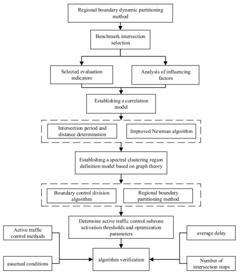
Figure 1.
Active traffic control zone delineation research idea chart.
2.1. Methods for Selecting Benchmark Intersections
The division of the urban road network intersection region must identify the benchmark intersection [18] based on the intersection road level, geographic location, and characteristics of the rapid diffusion of traffic status, which is used as a key point. The key point was then diffused to the surrounding intersections, and the benchmark intersection and its intersections that satisfied the correlation degree criterion were gradually consolidated into a control region.
The point where multiple streams of traffic, including straight, left-turn, and right-turn traffic, converge is known as the intersection. Furthermore, the flow of traffic at the intersections has a great influence on the condition of the regional road network. Therefore, the basic task of the regional partitioning method is the selection of benchmark intersections. The influence of road section traffic characteristics on the selection of benchmark intersections in the regional road network should be examined by specific analysis. In this paper, the average vehicle speed and traffic volume of the road section are selected as indexes to evaluate the traffic condition of the road, since the traffic condition of vehicles on the road section is mainly influenced by road condition, periphery vehicles, and speed limit. The traffic status of the intersection is comprehensively reflected by the lane saturation, which can reflect the traffic condition of the lane group. In accordance with the maximum membership degree concept, the maximum value of the saturation of all flows in an inlet lane is selected as the saturation of that inlet lane. The traffic state value of the whole intersection is calculated with the saturation of each inlet lane [19], which is used as an indicator to discern the operating state of the intersection. The concrete formulas are given in Equation (1).
In Equation (1): is intersection saturation state indicator. is the saturation of lanes flowing from the entrance road at intersection to intersection , is the saturation volume, which can be taken according to the literature [20], and is the effective green light time, is the maximum saturation of all flows on the entrance lane of intersection , is the cycle time of intersection , and is the number of entrance lanes of intersection .
The average maximum queue length is the average of the maximum queue length for each cycle, and its calculation model, as shown in Equation (2).
In Equation (2): is the cycle vehicle arrival flow rate, and is the duration of the red light (s). The queue length is the most logical indicator of traffic congestion and a crucial control and evaluation parameter for intersections.
The ratio of the section length to the total time taken for the vehicle to drive through the section is known as the average travel speed , as shown in Equation (3).
In Equation (3): is the length of the road section (m); is the hourly traffic volume of the road section during the survey time (pcu/h); is the travel time required for the vehicle passing the road section during the survey time. The average travel speed accounts for potential stopping delays, which can more accurately reflect the operational status of vehicles on a particular road stretch at a specific time. It is also a comprehensive indication that reflects the saturation of the road.
In this paper, the dynamic traffic parameters and static roadway indicators influencing the traffic state are considered in order to obtain a more realistic traffic operation condition of the road network. The intersection’s queue length, capacity, lane saturation, and average vehicle speed were selected as indicators to evaluate the operating status of the intersection. Thus, an intersection status indicator evaluation model is established, as shown in Equation (4).
In Equation (4): is the state value of the regions, is the model parameter between (0,1), and , and are intersection and , respectively, is the average speed of road section (m/s), is the maximum speed limit of the road section (m/s), is the actual flow of road section (pcu/h), is the capacity of road section (pcu/h), is the queue length of intersection (m), is the road load weight for intersection . is the fixed length. The value of is obtained according to the urban road engineering design specifications.
2.2. Integrated Correlation Degree Model of Boundary Definition-Related Indicators
A pivotal ring of an area boundary definition is the construction of a correlation model, which would be utilized to express quantitatively the suitability of adjacent intersections being divided into the same control region.
The partitioning of active traffic control subareas, the clarification of the elements that influence subarea partitioning, and the establishment of a correlation degree model for adjacent intersections, are all necessary. Many scholars have summarized the main factors affecting the correlation between intersections, which are mainly divided into dynamic and static factors, including traffic flow, signal period, green ratio, vehicle dispersion characteristics, intersection spacing, etc. The Whitson model from the American Manual of Traffic Control and its modifications are usually used to calculate the correlation between intersections, as shown in Equation (5).
In Equation (5): is the correlation of adjacent intersections, is the average travel time from upstream to downstream intersection (s); is the maximum flow rate from upstream intersection (pcu/s); is the flow rate of each inlet lane at the downstream intersection (pcu), in which is the number of lanes at the downstream intersection, and is the starting value of 1 for the number of flow directions from the upstream to the downstream intersection.
With the addition of capacity and the effect of vehicle dispersion on journey time, based on the Whitson model, the study further corrects the prior model. Thus, the correlation degree model for adjacent intersections under active traffic control is established, as shown in Equation (6).
In Equation (6): is the roadway correlation between upstream and downstream intersections, is the dispersion coefficient of the Robertson’s model, which is recommended to be 0.1–0.15, is 0.8 times of the average vehicle travel time between the two cross-sections (h), is the crossing capacity (pcu/h), is the upstream intersection capacity of intersection (pcu/h), is the maximum flow rate from the upstream intersection (pcu/h), is the downstream intersection traffic volume for each entrance lane (pcu/h).
3. Models for Dynamically Defining Regional Boundaries
To minimize the further spread of traffic congestion to adjacent intersections, the spatial-temporal variation characteristics of the traffic status of the road network are comprehensively considered in this paper, and a correlation analysis of the indicators connected to the boundary definition is performed. The spectral clustering approach is then used to dynamically construct the road network boundary based on the preliminary definition.
3.1. Preliminary Definition of Regional Boundaries
The intersection period and intersection spacing are determined as division principles by analyzing the factors influencing the correlation degree of intersections in order to alleviate the pressure of the subsequent algorithm. The traffic network’s intersections are then screened with the benchmark intersection as the center. Then, the improved Newman method [21] is used to define the control area boundaries in advance.
- (1)
- Intersection cycle
Differences between adjacent intersection cycles can affect the coordinated control. Different adjacent intersection cycles can lead to inefficient traffic flow through multiple intersections in a continuous manner in a condition of timing control coexisting with non-inductive and inductive control. Many traffic control systems currently divide traffic control subzones based on the length of the signal cycle. The essence is that the optimal cycle length of signals at adjacent intersections is similar (the cycle difference is less than seconds), which indicates that their traffic situations are similar. In this case, the signal coordination control is implemented in the intersection merged into a subdivision. Then, the total delay of each intersection after merging can be made smaller than the total delay before merging. To study the relationship between the cycle length and the traffic conditions determined by field observations and surveys, the t-value should also be based on the actual local situations.
- (2)
- Intersection distance
The spacing between adjacent intersections has an impact on coordination control. If the spacing is too small, the intersection vehicle queue will overflow; if the spacing is too long, the traffic flow dispersion will be severe, and the vehicle will not be able to travel continuously through the intersection. As a result, the intersection distance restriction conditions range from 200 m to 1200 m, based on experience.
In the preliminary definition, this paper is used to improve the Newman algorithm. First, the road network is initially divided into n communities, and each node in the network of communities represents a community, denoted as . The n-order symmetric matrix is defined as , for which is the edge weights of the edges connected between community and community , indicating the proportion of the internal edge weights of the community in the total edge weights of the network. The sum of the elements of each row of the matrix is , which represents the proportion of the edge weights of the internal nodes of the community connected to the external nodes to the total edge weights of the network. represents the sum of all elements of the matrix . This obtains the modularity of the entitled network as shown in Equation (7).
In Equation (7): is the modularity, is the total edges of community as a proportion of the sum of the edge weights in the total edge weights of the network. Tre is the sum of the diagonal elements of the matrix , which represents the proportion of the internal edge weights of the community in the total edge weights of the network. The community module degree must be at its maximum in a certain community partitioning procedure for the partitioning result to be optimal, and at that point the range of values is often between 0.3 and 0.7 [22].
The algorithm considers the correlation characteristics between the nodes of the network, and the edge weights between the nodes characterize the correlation degree between the nodes, so the elements in the auxiliary matrix and the elements in the array are improved, as shown in Equations (8) and (9).
In Equations (8) and (9): is the edge weight between node and node .
The Newman algorithm is applied to partition the regional road network, and the steps are as follows:
- (1)
- By turning intersections into nodes and the road segments between them into edges, the complexity of the supplied traffic network is simplified;
- (2)
- The traffic information at the network’s nodes and edges is collected and tallied, then it is substituted into the correlation degree calculation model to determine the correlation degree between adjacent intersections;
- (3)
- The nodes are divided into separate communities by the initialized community network;
- (4)
- The array and the auxiliary matrix , which contains all of the entries and , are defined and initialized;
- (5)
- The combined pair of nodes connected by edges is used to calculate the update modularity increment as shown by Equation (7);
- (6)
- As the mergers are carried out, the procedure (5) is continued until the network is fully integrated. The community network is divided as a result, and the best community networks may be created by choosing the value that maximizes modularity.
The road traffic network is a typical complex network, and by combining the community partitioning algorithm in complex networks for dynamic control, subzone partitioning is both feasible and superior. The algorithm calculates that the number of subregions is six, which corresponds to a maximum modularity of 0.6311. The specific partition is shown in Figure 2.
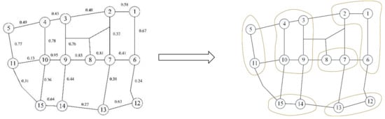
Figure 2.
The diagram of the Newman algorithm region partitioning for active traffic control.
In this paper, the second definition is applied using the spectral clustering algorithm, which integrates the efficiency and accuracy of the improved Newman algorithm for edge-weight analysis to rapidly and precisely divide the region boundary based on the initial definition.
3.2. Proposed Regional Boundary Definition Method Based on Spectral Clustering
The regional boundary definition uses a graph theory-based spectral clustering algorithm, which can cluster in any sample and converges to the optimal solution compared to traditional clustering methods. The essence of the algorithm is that the clustering is converted into an optimal partition of the graph, which is diffused to the periphery in a two-dimensional space to obtain the optimal solution.
Based on the spectral clustering algorithm of graph theory, the research creates a subzone dynamic partitioning model of the critical congestion points [23] and employs saturation as the partitioning criteria of congestion, where flow is the most intuitive indication of the intersection traffic status. The degree of saturation similarity was utilized to quantitatively describe how comparable the traffic operation levels were at various nodes [24].
The algorithm constructs the road network weighted graph , the set of intersections , and the set of road sections . Then, the weighted graph is partitioned into two traffic control regions, and , satisfying , . The road section weights of adjacent intersections and consider the traffic correlation, saturation similarity, and road section blockage indexes, as shown in Equations (10)–(12).
In Equation (10) to Equation (12): is the traffic correlation. , is the retardation coefficient, based on actual traffic data and road network structure, and is taken as 0.15, is taken as 4 according to experience, and are the saturation of intersection and , respectively, is the saturation similarity, is the roadway blocking indicator, is the intersection queue length, is the functional area length of the road section, including perception response, deceleration distance, and platoon queue length, and its value is based on the actual traffic data. is the road section flow between intersection and intersection . is the road section flow between intersection and intersection , is the weighting coefficient, taking the value range (0, 1). The degree of influence of actual intersections and road sections on road network congestion is determined according to the multi-factor statistical method. Based on the ratio of the capacity to the actual flow in key lanes, it is possible to calculate the intersection saturation, abbreviated as and .
Firstly, to determine the OD paths of the road network in the region for each time period and the traffic volume of each intersection for each time period, adopt the road segment correlation of adjacent intersections as its clustering index, in which the threshold value of the correlation should be set in advance. Secondly, to determine the correlation model based on the intersection traffic situation, model the segment weights considering segment correlation, saturation similarity, and blockage indicators. Subsequently, a similarity matrix is established by using the spectral graph theory and combining the saturation of intersections to achieve the maximum traffic correlation and the closest similarity in the control area for the division objective. Finally, the nodes are defined by using the function to find the second eigenvalue of the M matrix, and the spectral clustering algorithm divides the steps as follows:
- (1)
- Division of the cut set control area
The boundary region definition is to divide the intersections with higher correlation and similarity into the same control region, which is to form a control region set with higher similarity and lower similarity rules. Then, the maximum and minimum cut set’s spectral graph division is selected as the objective, and the objective function is shown in Equations (13)–(15).
In Equations (13)–(15): is the set of control areas, is the edge weight between intersection and intersection , is the total edge weight of all intersections in the control area of . The M-cut set should not only minimize , but also maximize and , which is conducive to a reasonable cut set to divide the control area and achieve results consistent with the objective.
- (2)
- Similarity matrix
The similarity matrix is defined for its factors as shown in Equation (16).
In Equation (16): is each data sample point, generally . is an artificially set parameter, so the larger the value the more obvious the classification effect.
A similarity matrix model is constructed using the section weights of road section correlation, saturation similarity, and blocking indicators, as shown in Equation (17).
In Equation (17): is the similarity matrix, and are the maximum values of the saturation of each entrance lane of intersection and , respectively, means intersection is joined with intersection , and the value of is taken as 1 according to experience.
The degree matrix is a diagonal matrix with all degree values as diagonal elements, with the degree of the vertices equal to the sum of the elements of each row of the similarity matrix. The diagonal elements meet at Equation (18).
- (3)
- Road network node division
The matrix is constructed using the edge weights for the road network, and the resulting normalized matrix is then obtained, as shown in Equations (19) and (20).
In Equations (19) and (20): is the unnormalized matrix, is the normalized matrix, is the random wandering matrix.
The minimization function is transformed into solving for the second minimum eigenvalue of the matrix using spectral graph theory, as shown in Equation (21).
In Equation (21): is the eigenvalue, is the feature vector that corresponds to the eigenvalues , and the final dimensional feature matrix is created by normalizing the matrix made up of by rows.
The vector is a feature vector that corresponds to the second eigenvalue, which represents an optimal graph division solution. The road network nodes are divided by the values in the vector. According to the heuristic rule, the elements of the vector are arranged in ascending order and searched one at a time. Each search divides the items of the vector into two classes. There are classified results. classified results are available. Each scheme’s value is identified, and as a consequence of subregion partitioning, the scheme with the lowest value is chosen.
The benchmark intersection is utilized as the center to preliminarily define the surrounding intersections, and the spectral clustering algorithm is employed to obtain the range constraint of the control region division, all based on the PI value. Then, the changes in the traffic flow parameters of the road network are dynamically adjusted to obtain the control area applicable to the active traffic control and the specific division flow chart, as shown in Figure 3.
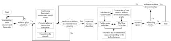
Figure 3.
Dynamic regional definition flow chart.
4. Model Validation and Discussion
To evaluate the effectiveness of the dynamic area definition approach, which is compared to the traditional intersection cluster hierarchical clustering algorithm [11] and the boundary control subzone delineation method [14]. As illustrated in Figure 4, the approach chose a city’s main metropolitan road network as an example in space, which includes 15 signal intersections and 29 road sections, with road network structures and intersection distances ranging from 160 to 950 m. The transition phase from flat to peak is selected for algorithm validation in time.
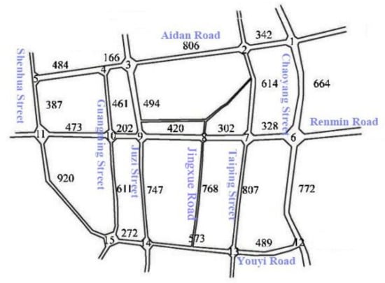
Figure 4.
Regional road network diagram.
In the simulated road network, every signalized intersection employs a standard four-phase release approach. The experimental area’s road network is set to a free-flow speed of 45 to 50 km/h, with the data detection points of each road section positioned in the middle of the road section and each road section placed in the delay detection section. The input flow of all boundary sections inside the experimental region satisfies the demand for traffic, and active traffic control is engaged in accordance with the established queue length and speed thresholds. In this traffic demand scenario, the road network volume gradually increases and then decreases, simulating the evolution of regional traffic flow from low peak to congestion peak.
The method performed in this paper utilized Equation (4) to determine intersection 1, intersection 9, intersection 11, intersection 12, and intersection 15 as the benchmark intersection, and then employed the spectral clustering algorithm to determine the control boundary. Then, for each control subzone, the queue length and speed criteria can be calculated using cluster analysis [13]. The indicator thresholds can then be used to determine when active traffic control begins. Subsequently, the detectors are then installed based on the determined queuing threshold, which is utilized to receive the active traffic control trigger threshold. Finally, simulation verification is performed using the VISSM simulation program to provide average vehicle delays and intersection numbers of stops on the road network in order to assess the effectiveness and reasonableness of the area boundary division method.
Using Equation (6) to determine the correlation value of all road sections in the road network, as shown in Table 1.

Table 1.
Path correlation value.
Then, the similarity matrix of each intersection is calculated, combined with the spectral clustering algorithm to calculate the vector, and then searched according to the heuristic rules to obtain the optimal congestion control boundary division scheme of the road network, as shown in Figure 5a. The regional boundary is divided using the intersection cluster hierarchical clustering algorithm based on multiple characteristic factors and the boundary control subzone division method, and the division results are shown in Figure 5b,c. Next, the active traffic control situation is analyzed using each of the three boundary delineation results to determine which division method is most suitable for active traffic control.
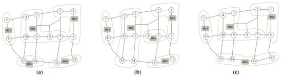
Figure 5.
Control boundaries of spectral clustering algorithm (a), intersection group hierarchical clustering algorithm (b), and boundary control subzone delineation method (c).
The whole road network adopts arterial coordination control, and this paper will adopt an active traffic control strategy for each control area separately on this basis. The active traffic control strategy is applied to each control area separately, which is based on the idea of interception + flow limitation to balance the surrounding traffic pressure, and then the main control intersection is analyzed for the non-variable cycle with comprehensive consideration of upstream and downstream traffic pressure. The phase variations are increased on the basis of regulating the green light duration within the phase, so that the green light within the phase can be used efficiently. The optimization of key intersections is carried out while coordinating upstream and downstream to equalize the traffic load between intersections and achieve coordinated regional control.
The active control strategy’s switching scheme determines the maximum and minimum green times of the key phase in detail. It evaluates whether or not the key phase is run before deciding whether or not to switch the phase based on the maximum green time and minimum green time, which affects the green light allocation for this cycle and the next. On the premise of ensuring that the switching scheme has less impact on the current traffic flow, with the specific switching strategy depicted in Figure 6, the active traffic control scheme is used to alleviate the initial road congestion.
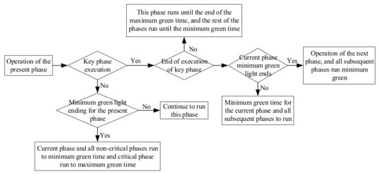
Figure 6.
Active traffic control switching flow chart.
As shown in Table 2, Table 3 and Table 4, the control boundary, common period, and phase difference of each region need to be calculated before the implementation of the active traffic control strategy.
Table 2.
Common period and phase difference within the control boundary under the spectral clustering algorithm.
Table 3.
Common period and phase difference within the control boundary under the intersection group hierarchical clustering algorithm.
Table 4.
Common period and phase difference within the control boundary under the boundary control subarea division method.
The path correlation degree is used to determine the coordinated direction based on the control parameters from Table 2, Table 3 and Table 4, to optimize phase difference and phase sequence. The total simulation time is 36,000 (s), and the average of 10 simulations is used. The average delay, average number of stops, queue length, and travel time under the road network are selected as the evaluation parameters, and the data sampling interval is 600 s. A comparison of the effects of different division methods is shown in Table 5.
Table 5.
Comparison of the effect of regional division methods.
As shown in Table 5, implementing the spectral clustering algorithm to execute the active traffic control strategy under the control area division improved the average traffic delay, the average number of vehicles stopped, the average travel time, and the queue length over the whole road network. Among them, the method reduces the average delay of the road network by 4.8%, the average stop of a vehicle by 12.1%, and the average travel time by 11.2% compared with the intersection clustering algorithm. The approach proposed decreases by 10.3%, 31.7%, and 30.3% when compared to the boundary control subdivision method, respectively. As a result, the approach of the dynamic area boundary definition used in this work is more applicable to active traffic control methods.
There are research methods that have not achieved optimal results when the traffic control system is implemented in combination with the subzone partitioning method. Additionally, although the method in this paper has some limitations, the victory lies in the traffic control subarea scheme applied to the corresponding traffic control system. This method enables it to coordinately control traffic flows in the control subregion that have similar traffic characteristics. As the saturation approaches the oversaturation threshold, the signal control effect may be impacted. Therefore, in order to ensure smooth operation inside the subzone, the active control approach can be used to divert traffic flows in the subzone prior to oversaturation. The method also provides a new idea for the control region partitioning method, which can study the corresponding control partitioning for the existing urban traffic control system. So, it offers practical guidance for the design of traffic signal control schemes.
5. Conclusions
This paper primarily supports the active traffic control method and establishes the active traffic control system’s boundary index correlation degree model, which takes into account influencing factors such as intersection spacing, capacity, queue length, intersection flow, and traffic dispersion, as well as realizing the dynamic division of area boundaries using the spectral clustering algorithm. This region boundary dynamic definition method can delineate intersections with stronger correlation into the same area, distributing the congestion degrees of road sections within the area evenly and facilitating the implementation of active traffic control schemes while reducing the number of vehicle stops and control delays on the road sections. However, the proposed dynamic division of regional borders in this paper ignores mutual interference between multiple control regions, and the control scheme implementation ignores regional active coordination control of the whole road network. The approach is intended for the active traffic control method of area dynamic division, based on the active traffic control area’s traffic flow characteristics, taking into account the characteristics of the road section and intersection traffic complexity under the traffic medium saturation (0.6–0.8). The approach has some pertinence, but it also has strict limitations and is not appropriate for all traffic signal control strategies. In addition, although the algorithm can produce high-quality partitions in a relatively short time, the vector computation is time-consuming if very large road networks are involved. The next stage will be to carry out research into the areas of regional boundary interference and regional active coordination control. In further research, the basic characteristics of traffic control methods and the traits of traffic flow are merged to adapt the model’s parameters and to lessen the computing burden. Thus, it is possible to make both the traffic control approach and the subzone classification method universal.
Author Contributions
Conceptualization, Y.X. and W.L. (Wenqing Li); methodology, W.L. (Wenqing Li); software, Y.L.; validation, Z.Z., W.L. (Wenqing Li), and Y.L.; formal analysis, Y.X.; investigation, W.L. (Weidong Liu); resources, Y.X.; data curation, W.L. (Wenqing Li); writing—original draft preparation, W.L. (Wenqing Li); writing—review and editing, W.L. (Wenqing Li); visualization, Y.X.; supervision, Y.X.; project administration, Y.X.; funding acquisition, Y.X. All authors have read and agreed to the published version of the manuscript.
Funding
Project of Liaoning Provincial Education Department: Research on Evaluation Method of Urban Regional Road Network Structure Based on Supply and Demand (LJKZ0590); National Natural Science Foundation of China: Vehicle Static Scheduling and Dynamic Control Method under Overlapping Operating Ranges of High Frequency Bus Lines (71771062).
Institutional Review Board Statement
Not applicable.
Informed Consent Statement
Not applicable.
Data Availability Statement
Not applicable.
Conflicts of Interest
The authors declare no conflict of interest.
References
- Whitson, R.H.; White, B.; Messer, C.J. A Study of System Versus Isolated Control as Developed on the Mockingbird Pilot Study; Texas Transportation Institute, Federal Highway Administration: Dallas, TX, USA, 1973; pp. 1–495. [Google Scholar]
- Zhou, Z.; Lin, S.; Xi, Y.F. A dynamic network partition method for heterogenous urban traffic networks. In Proceedings of the 2012 15th International IEEE Conference on Intelligent Transportation Systems, Anchorage, AK, USA, 16–19 September 2012. [Google Scholar]
- Yuxuan, J.I.; Nikolas, G. On the spatial partitioning of urban transportation networks. Transp. Res. Part B 2012, 46, 1639–1656. [Google Scholar]
- Lowrie, P.R. Scats, Sydney Co-Ordinated Adaptive Traffic System: A Traffic Responsive Method of Controlling Urban Traffic; Roads and Traffic Authority NSW: Darlinghurst, Australia, 1990; pp. 1–28. [Google Scholar]
- Song, L.J.; Zhu, J.Z.; Liu, X.J.; Jing, C.H.E.N.; Kai, X.I.A.N. Optimization method of traffic analysis zones division in public transit corridors. J. Transp. Syst. Eng. Inf. Technol. 2020, 20, 34–40. [Google Scholar]
- Batista, S.F.A.; Leclercq, L.; Geroliminis, N. Estimation of regional trip length distributions for the calibration of the aggregated network traffic models. Transp. Res. Part B Methodol. 2019, 122, 192–217. [Google Scholar] [CrossRef]
- Keyvan-Ekbatani, M.; Yildirimoglu, M.; Geroliminis, N.; Papageorgiou, M. Traffic signal perimeter control with multiple boundaries for large urban networks. In Proceedings of the 16th International IEEE Conference on Intelligent Transportation Systems (ITSC 2013), Hague, The Netherlands, 6–9 October 2013. [Google Scholar]
- Liwei, H.U.; Xueting, Z.H.A.O.; Jinqing, Y.A.N.G.; Suhang, Z.H.A.N.G.; Zijian, F.A.N.; Xiufen, Y.I.N.; Zhi, G.U.O. Urban traffic congestion mitigation and optimization study based on two-level programming. J. Transp. Syst. Eng. Inf. Technol. 2021, 21, 222–227+234. [Google Scholar]
- Feng, Y.J.; Shan, M.; Le, H.C.; Zhang, G.J.; Yu, L. Subarea dynamic division algorithm based on green wave coordinated control. Control. Theory Appl. 2014, 31, 1034–1046. [Google Scholar]
- Shen, G.J.; Yang, Y.Y. A dynamic signal coordination control method for urban arterial roads and its application. Front. Inf. Technol. Electron. Eng. 2016, 17, 907–918. [Google Scholar] [CrossRef]
- Qu, D.; Jia, Y.; Liu, D.; Yang, J.; Wang, W. Dynamic partitioning method for road network intersection considering multiple factors. J. Jilin Univ. (Eng. Technol. Ed.) 2019, 49, 1478–1483. [Google Scholar]
- Lan, H.; Wu, X. Research on Key Technology of Signal Control Subarea Partition Based on Correlation Degree Analysis. Math. Probl. Eng. 2020, 2020, 1879503. [Google Scholar] [CrossRef] [Green Version]
- Yiming, B.I.E.; Linhong, W.A.N.G.; Xianmin, S.O.N.G. Strategy of dynamic traffic control subarea partition in urban road network. China J. Highw. Transp. 2013, 26, 157–168. [Google Scholar]
- Lan, L.I.U.; Weike, L.U.; Guojing, H.U.; Feng, W.A.N.G.; Junsong, Y.I.N. Spatial partitioning of traffic networks for boundary flow control. China J. Highw. Transp. 2018, 31, 86–196. [Google Scholar]
- Saedi, R.; Saeedmanesh, M.; Zockaie, A.; Saberi, M.; Geroliminis, N.; Mahmassani, H.S. Estimating network travel time reliability with network partitioning. Transp. Res. Part C Emerg. Technol. 2020, 112, 46–61. [Google Scholar] [CrossRef]
- Dimitriou, L.; Nikolaou, P. Dynamic partitioning of urban road networks based on their topological and operational characteristics. In Proceedings of the 2017 5th IEEE International Conference on Models and Technologies for Intelligent Transportation Systems (MT-ITS), Naples, Italy, 26–28 June 2017. [Google Scholar]
- Ezaki, T.; Imura, N.; Nishinari, K. Towards understanding network topology and robustness of logistics systems. Commun. Transp. Res. 2022, 2, 100064. [Google Scholar] [CrossRef]
- Pignataro, L.J.; McShane, W.R.; Crowley, K.W.; Lee, B.; Casey, T.W. Traffic Control in Oversaturated Street Networks; Transportation Research Board: Washington, DC, USA, 1978; pp. 1–152. [Google Scholar]
- Baichuang, L.U.; Xin, W.A.N.G.; Jieyi, Y.A.N.G. The traffic status evaluation of urban regional road networks considering structural differences. J. Chongqing Univ. Technol. (Nat. Sci.) 2022, 36, 50–58. [Google Scholar]
- Bing, W.U.; Ye, L.I. Traffic Management and Control; China Communication Press: Beijing, China, 2005; pp. 56–141. [Google Scholar]
- Tian, X.J.; Yu, D.X.; Zhou, H.X.; Xing, X.; Wang, S.G. Dynamic control subdivision based on improved Newman algorithm. J. Zhejiang Univ. (Eng. Sci.) 2019, 53, 950–956+980. [Google Scholar]
- Wang, L.; Luo, J. Research on Regional Traffic Division Based on Improved Relevance Degree and Newman Algorithm. Comput. Eng. Appl. 2021, 1–9. Available online: http://kns.cnki.net/kcms/detail/11.2127.tp.20210714.1450.010.html (accessed on 3 August 2022).
- Zhang, Z.; Yang, X. Analysis of highway performance under mixed connected and regular vehicle environment. J. Intell. Connect. Veh. 2021, 4, 68–79. [Google Scholar] [CrossRef]
- Xu, J.M.; Yan, X.W.; Jing, B.B.; Wang, Y.J. Dynamic Network Partitioning Method Based on Intersections with Different Degree of Saturation. J. Transp. Syst. Eng. Inf. Technol. 2017, 17, 145–152. [Google Scholar]
Publisher’s Note: MDPI stays neutral with regard to jurisdictional claims in published maps and institutional affiliations. |
© 2022 by the authors. Licensee MDPI, Basel, Switzerland. This article is an open access article distributed under the terms and conditions of the Creative Commons Attribution (CC BY) license (https://creativecommons.org/licenses/by/4.0/).