Electric Vehicle Charging Station Location Model considering Charging Choice Behavior and Range Anxiety

Abstract

Electric vehicles (EVs) have the advantages of low pollution, low energy consumption, and high energy efficiency, so they are highly valued by governments, enterprises, and consumers. However, the promotion and use of electric vehicles is restricted to a certain extent because of their limited range. This paper selects electric vehicle intercity medium- and long-distance travel as the research object, and takes the classical flow-capturing location problem as the theoretical basis for the expressway network or national highway network. This paper also considers the driver’s charging choice behavior and range anxiety, studies the electric vehicle charging station location problem, establishes the charging station location model, and uses the Tabu search algorithm to solve the problem. Finally, the effectiveness of the model and algorithm is verified by empirical analysis. The results show that the charging station location model considering the driver’s charging choice behavior and range anxiety performs better.

1. Introduction

There are many kinds of electric vehicles, which can be divided into fuel cell vehicles (FCVs), hybrid vehicles (HVs), and battery electric vehicles (BEVs). The electric vehicles mentioned in this paper especially refer to battery electric vehicles. Compared with traditional internal combustion engine vehicles, electric vehicles bring many practical and environmentally friendly advantages to individuals and society, including better maneuverability, lower noise, and less environmental impact. Thus, it can be seen that the popularity of electric vehicles helps to reduce people’s dependence on fossil fuels and improve the utilization rate of renewable energy. However, electric vehicles have the characteristics of high initial purchase cost, limited range, and long charging time, which affect the large-scale promotion and use of electric vehicles [1]. Therefore, the use of electric vehicles is often limited to short-distance travel within the urban area, such as for commuting, shopping, and entertainment, while intercity medium- and long-distance travel is less, and its applicable scope and convenience cannot be idealized. In order to better popularize and promote electric vehicles, increase the use frequency of electric vehicles in intercity medium- and long-distance travel, and extend their applicable scope, this paper focuses on their supporting facilities, such as electric vehicle charging stations. Scientific and rational planning and construction of charging stations to solve the problem of charging during travel can effectively ensure the smooth completion of electric vehicles.

With the emergence and development of the electric vehicle industry, the location of charging facilities has gradually become focus of research. This paper studies the locations of charging stations on expressway networks or national highway networks, based on the flow-capturing location model (FCLM). In general, the requirements of traditional location models (such as the maximum coverage model) are generated by network nodes, while Hodgson et al. [2] discussed the problem of demand generation on the path, and proposed and studied how to determine a given number of service station locations in the network in order to maximize the FCLM of the total traffic through the service stations. Kuby and Lim [3] extended the FCLM and proposed the flow-refueling location model (FRLM), which takes into account the situation of multiple instances of energy refueling in a single trip. In order to establish the FRLM, Kuby and Lim introduced a combination of feasible charging facilities, and selected the optimal combination of charging facilities to make the path feasible through the external algorithm, so as to ensure the feasibility of the travel path in the network. After that, Kuby and Lim extended the FRLM to study the addition of nodes to the road section [4] and the offsetting of the FRLM path [5]. Based on the offsetting of the FRLM path, Guo et al. [6] established the range anxiety flow attenuation function, which was used to represent the flow attenuation in the offset path and to study the location of electric vehicle charging stations. Based on the FRLM, Chung and Kwon [7] established a multicycle optimal charging station location model for strategic charging station location planning, and carried out an example analysis based on the actual traffic flow data of the Korean expressway network in 2011. Capar et al. [8] proposed a new generalized FRLM, which takes into account the distance travelled by the vehicle from the origin to the destination. This new model is based on covering the arc containing each path, which is more efficient than the previous FRLM. By studying the charging logic of electric vehicles in the network, Xu et al. [9] established a compact mixed-integer nonlinear programming model based on the offsetting of the FRLM path. This model does not need to consider the pre-generated charging path and charging service combination, and it is more efficient than the offsetting of the FRLM path. Based on the FRLM, and considering the return of travelers, Zhu [10] studied the location of charging stations for many types of electric vehicles.

In the research of charging station location, most of the existing studies consider the location problem from the position of the supplier, but seldom from the position of driver. This paper studies the location of charging stations from two perspectives of supply and demand, considering the number restrictions and the path feasibility constraints of charging stations at the supply level, and the charging choice behavior and range anxiety of drivers at the demand level. According to the research of expressway networks and national highway networks, the charging station location model is constructed based on the FCLM.

2. Problem Statement

The research object of this paper is the intercity medium- and long-distance travel of electric vehicles on the expressway or national highway networks. The research object only considers direct current (DC) fast-charging stations. Based on the research of Kuby and Lim [3], the location of the charging stations in this paper takes into account the charging demand of users throughout the whole return travel process. For intercity medium- and long-distance travel, because of the longer travel distance, drivers must consider the problem of vehicle charging in the process of driving, and drivers are often affected by range anxiety in the process of travel. The influence of the driver’s charging behavior and range anxiety on the location of the charging station is considered in the location planning, making it more in line with the actual travel of the driver. The reasonable placement of charging facilities can effectively alleviate the range anxiety of drivers in the process of travel and, thus, promote the popularity and application of electric vehicles.

2.1. Charging Selection Behavior Based on Cumulative Prospect Theory

In the field of transportation, there is a precedent for using cumulative prospect theory to model irrational choice behavior. For example, cumulative prospect theory has been applied to the study of choice behavior under uncertain conditions, such as path selection, commuting departure time selection, transfer mode selection, etc. These studies have successfully used cumulative prospect theory to describe people’s bounded rationality and risk preference when making decisions. Gao, Schwanen, and Xu [11,12,13] compared the cumulative prospect theory with the expected utility theory, and their results showed that cumulative prospect theory is a better method to simulate the decision-making behavior of travelers. In this paper, citing the research of Hu et al. [14], according to cumulative prospect theory, the cumulative prospect value $V\left(r_{i,next}\right)$ of charging and not charging is calculated using the following Equation (1):

$$V\left(r_{i,next}\right)={\displaystyle \sum _{i=0}^n{\pi }_i^{+}\left(p_i\right)}v\left(C_i\left(r_{i,next}\right)\right)+{\displaystyle \sum _{i=-m}^{-1}{\pi }_i^{-}\left(p_i\right)}v\left(C_i\left(r_{i,next}\right)\right)$$

(1)

where $\pi \left(p\right)$ is the cumulative decision weight function of charging selection behavior, and $r_{i,next}$ is the remaining range when the electric vehicle arrives at the next charging station of node i. The charging selection behavior value function $v\left(C\left(r_{i,next}^k\right)\right)$ or charging cost function $C\left(r_{i,next}^k\right)$ is sorted in increasing order, and the ordinal k of the result is converted to ordinal i; that is, $v\left(C_i\left(r_{i,next}\right)\right)$, $C_i\left(r_{i,next}\right)$, and $-m\le i\le n$. When the value of the result is “gain”, $0\le i\le n$; when the value of the result is “loss”, $-m\le i\le n$. The superscript “+” is used to denote the result of gain, the superscript “−” indicates the result of loss, and “0” indicates a neutral result. When the driver decides to charge, the cumulative foreground value is $V_{ch\arg e}\left(r_{i,next}\right)$, and when not charging, the cumulative foreground value is $V_{notch\arg e}\left(r_{i,next}\right)$. The driver of the electric vehicle makes a charging decision according to the calculated cumulative prospect value of charging and not recharging. When $V_{ch\arg e}\left(r_{i,next}\right)\ge V_{notch\arg e}\left(r_{i,next}\right)$, the driver will make the decision to charge; otherwise, they will choose not to charge. When the driver makes a charging decision, the remaining range of the electric vehicle will be updated.

2.2. Analysis of Driver’s Range Anxiety and Charging Selection

Because of the limited range of electric vehicles, drivers often suffer from the psychological pressure of “range anxiety” in the real driving process [9]. Range anxiety refers to the driver’s worry that the battery of the electric vehicle will be completely exhausted during the trip, resulting in breaking down and not being able to complete the trip smoothly [15]. The imperfect charging facilities of electric vehicles also aggravate the range anxiety of drivers. This section discusses this problem based on the research of Xu et al. [9], Xu et al. [16], and Yang et al. [17], who found that electric vehicle drivers’ range anxiety is largely affected by the remaining state of charge (SOC), and that there is a negative correlation between them. The lower the residual SOC of electric vehicles, the higher the driver’s range anxiety. Xu et al. [16] noted that the relationship between range anxiety and residual SOC is roughly a convex function; that is, the slope of range anxiety increases with the decrease in residual SOC. Franke et al. [18] leased 40 electric vehicles to sample users for a six-month field study. Their research showed that the driver has a comfort range threshold when driving the electric vehicle. When the remaining SOC is higher than the comfort range threshold, the driver will not experience range anxiety, but when the remaining SOC is lower than the comfort range threshold, the driver will begin to experience range anxiety.

With the increase in the remaining SOC, the range anxiety of electric vehicle drivers will gradually decrease from the maximum value R_max; until the remaining SOC decreases to the comfort range threshold L_comf, the range anxiety will be reduced to 0. The relationship between range anxiety and the remaining SOC of electric vehicles is transformed into the relationship between range anxiety and driving mileage. When the electric vehicle is fully charged from the starting point, the mileage is l = 0. For simplicity, assume that the electric vehicle discharges linearly at a constant speed, and that the distribution of the remaining SOC and mileage l is a linear distribution, as shown in Equation (2):

$$SOC\left(l\right)=DR-\mu l$$

(2)

where μ is a linear parameter.

In the SOC(l) function, when SOC drops to L_comf, $l_{cmof}=(DR-L_{comf})/\mu$. When the mileage is greater than l_comf, range anxiety will increase from 0. Range anxiety increases with the increase in mileage, as does the slope, and there is a convex function relationship between them. When the mileage l of the electric vehicle reaches the range DR, the range anxiety reaches the maximum value R_max.

Based on the research of Xu et al. [9], the convex function R(l) can be used to express the relationship between the driver’s range anxiety and driving mileage. There are many types of range anxiety function R(l), and we can choose one of the two most common types to describe the range anxiety function: power function, and exponential function. In this paper, the range anxiety function R(l) is as shown in the following Equation (3):

$$R\left(l\right)=\left\{\begin{array}{l}0,0\le l<l_{cmof}\\ \frac{R_{\max }}{{\left(\frac{DR}{\mu }-l_{cmof}\right)}^2}{\left(l-l_{cmof}\right)}^2,l_{cmof}\le l\le \frac{DR}{\mu }\end{array}\right.$$

(3)

According to the research on comfort range threshold by Franke et al. [18], the driver’s comfort range threshold was set to $L_{cmof}=30km$; α is a constant, and the image of the function can be determined by calibrating the parameter α. Figure 1 shows the image of the power function under different parameters, in which $DR=300km,\mu =1$.

When using the power function to describe range anxiety, no matter how α changes, the R_max reaches the maximum value of 1. When using the exponential function to describe range anxiety, the maximum value R_max increases with the increase in α. Therefore, using the power function to describe range anxiety has a certain advantage in terms of dimensional unity. These diagrams can help drivers to effectively understand the changes in range anxiety. In addition, the slope of range anxiety can be controlled by replacing e in the exponential function with other constants.

Citing the research of Xu et al. [9], the cumulative range anxiety of the whole journey can be expressed as the accumulation of range anxiety over all charging path sections. The calculation Equation (4) of range anxiety $R_{cum}\left(r\right)$ is given in this paper as follows:

$$R_{cum}\left(r\right)=\left\{\begin{array}{l}0,L_{comf}\le r\le DR\\ \frac{R_{\max }}{3\mu L_{comf}{}^2}{\left(L_{comf}-r\right)}^3,0\le r\le L_{comf}\end{array}\right.$$

(4)

where r represents the remaining range of the electric vehicle when it reaches the end node of a charging path section. When r = 0, $R_{cum}\left(r\right)$ reaches its maximum value, and the maximum value is $R_{cum}{\left(r\right)}_{\max }=R_{\max }{L}_{comf}/3\mu$. In this paper, in order to facilitate the calculation and unify the dimensions, μ = 1, unless otherwise stated, and R_max is normalized to 1 in the numerical experiments. Throughout the whole travel process of the electric vehicle, the vehicle may arrive at the charging station many times and choose whether or not to charge, so the whole travel process is a multicycle driving process. When the electric vehicle arrives at the charging station and chooses to recharge, the driver’s range anxiety will be reset according to the rechargeable capacity, and if the electric vehicle is fully charged, the range anxiety will be reset to 0.

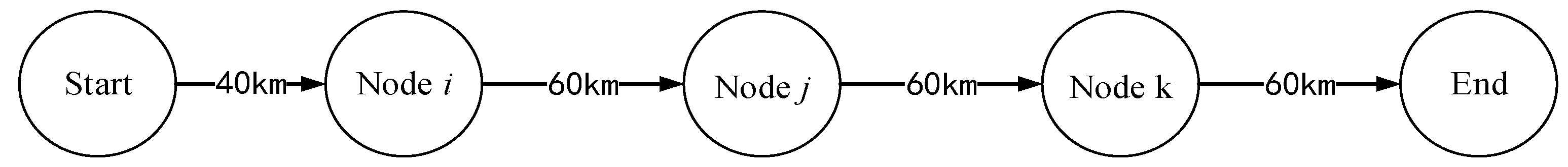
2.3. Feasibility Analysis of Electric Vehicle Path

Before establishing the charging station location model, it is necessary to analyze the feasibility of the electric vehicle in the path. The path feasibility of the electric vehicle is defined as follows: if the electric vehicle does not need to be recharged one or more times during the trip, the electric vehicle can arrive at the destination directly from the starting point, and it will not run out of power during the driving process, then origin–destination (OD) travel is feasible. Otherwise, if the electric vehicle runs out of power during the process of travel, then the electric vehicle cannot reach the next node and, thus, cannot complete the entire trip, so OD travel is not feasible. In the FRLM, the charge flow can be intercepted only when the path is feasible. In order to ensure the feasibility of the path, the FRLM uses an external algorithm to pre-generate the proper combination of charging facilities to ensure the feasibility of the path, and does not express the path feasibility constraints in the model. On the other hand, the pre-generated charging facility combination algorithm can easily cause insufficient memory in the process of operation, and it is more inconvenient in the process of use. Therefore, through the path feasibility study, this paper improves the FRLM and expresses the path feasibility constraints in the model to avoid pre-generating the combination of charging facilities, while ensuring the interception of feasible path flow.

By extending the research on the refueling logic of fuel vehicles in the linear path by Wang and Lin in 2009 [19], the charging logic of electric vehicles in the linear path can be determined. Figure 2 shows a simple example of electric vehicle travel, which can illustrate the spatial characteristics of electric vehicle charging.

Suppose that the total range of the electric vehicle is 100 km, the shortest path between the starting point and the destination is 220 km, and there are three nodes in the middle. Because the vehicle still has a 60 km range (more than half of the range) when it reaches node i, the driver will choose to use all of the electricity to reach node j, and a charging station should be set up at node j. When the vehicle arrives at node k from node j, the remaining power is only enough to drive 40 km, and cannot continue to reach the final destination. A charging station must therefore be set up at node k so that the driving distance can be extended at least 20 km to reach the destination.

The charging logic of the electric vehicle in the linear path can be obtained through the example in Figure 3. Assuming that nodes i and j are any two adjacent nodes on path q, then $\left(i,j\right)$ is a road section on path q; that is, $\forall i\in N_q,\left(i,j\right)\in A_q,q\in Q$.

The charging logic of an electric vehicle in a linear path can be described by the following statements:

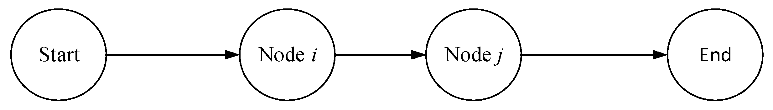
• If the vehicle can reach node i, this means that there is still range $r_i^q$ left when the vehicle arrives (or that the vehicle runs out of electricity when it arrives), as shown in Equation (5):

  $$0\le r_i^q\le DR,\forall i\in N_q,q\in Q$$

  (5)
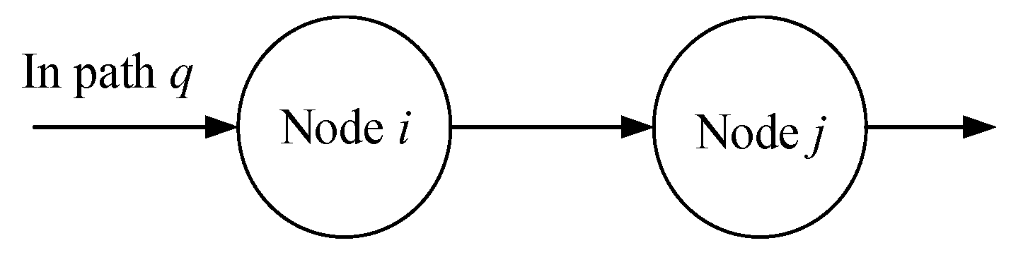
• If a charging station is not built at node i, the driver cannot charge here; if a charging station is built at node i, according to the charging selection behavior model, the driver will make a charging selection at this node, as shown in Equations (6) and (7):

  $$y_i^q=\left\{\begin{array}{l}1,if{V}_{ch\arg e}\left(r_{i,next}^q\right)\ge V_{notch\arg e}\left(r_{i,next}^q\right)\\ 0,if{V}_{ch\arg e}\left(r_{i,next}^q\right)<V_{notch\arg e}\left(r_{i,next}^q\right)\end{array}\right.,\forall i\in N_q,\left(i,next\right)\in E_q,q\in Q$$

  (6)

  $$x_i\ge y_i^q,\forall i\in N_q,q\in Q$$

  (7)
• The remaining range of the vehicle arriving at node j is the remaining range r_j of the vehicle at node i plus the increased mileage of the vehicle charging at node i, minus the distance between node i and node j, as shown in Equation (8):

  $$r_j^q=\left(r_i^q+y_i^q{c}_i^q\right)-l_{ij},\forall i\in N_q,\left(i,j\right)\in A_q,q\in Q$$

  (8)
• In the medium- and long-distance travel in the expressway network, the electric vehicle has less opportunity to charge than in the city, and the driver often recharges the vehicle when possible, so this paper assumes that if the vehicle is charged, it will be charged to DR. The increased mileage c_i of the vehicle charged at node i is shown in Equation (9):

  $$c_i^q=DR-r_i^q,\forall i\in N_q,q\in Q$$

  (9)
• If $r_j^q\ge 0$, this means that when the vehicle reaches node j, the vehicle still has remaining range and can move on. On path q, if $0\le r_i^q\le DR$ is known to satisfy $r_j^q\ge 0$ for any node i, this means that the OD trip is feasible; that is, $Y^q=1$. If $r_j^q<0$ means that the vehicle cannot reach the next node j, it also means that the OD travel is not feasible; that is, $Y^q=0$. There are many reasons for the infeasibility of OD travel, such as unreasonable layout of charging stations, faulty charging choices for drivers, long road distances exceeding the total range of electric vehicles, etc. If path q is not feasible, for the compactness of the model, a difference variable ${\Delta }_i^q$ is introduced to represent the amount of electricity that needs to be replenished from node i to node j, in addition to the normal power supply. If ${\Delta }_i^q>0$ in path q, then the OD is not feasible for q. At this point, there is Equation (10):

  $$r_j^q=\left(r_i^q+y_i^q{c}_i^q+{\Delta }_i^q\right)-l_{ij},\forall i\in N_q,\left(i,j\right)\in A_q,q\in Q$$

  (10)
  When OD is feasible for q, the above formula still holds, but ${\Delta }_i^q=0$.
• The cumulated range anxiety (CRA) of electric vehicle drivers between all OD pairs in the road network can be calculated by Equation (11):

  $$CRA={\displaystyle \sum _{q\in Q}{f}^q{Y}^q}\left[{\displaystyle \sum _{i\in N_q}{R}_{cum}\left(r_i^q\right)y_i^q+R_{cum}\left(r_{s\left(q\right)}^q\right)}\right]$$

  (11)

3. Model Building

3.1. Symbols and Decision Variables

The symbols and decision variables involved in modeling in this paper are shown in

Table 1. Symbols and descriptions of expressway network parameters.

Parameter Symbol	Parameter Description	Parameter Unit
G	An expressway network G = (N,A)	/
N	A collection of nodes in an expressway network, which is composed of N nodes.	/
A	Collection of road sections in an expressway network	/
i,j	Nodes i and j in an expressway network, $i,j\in N$	/
(i,j)	The section of an expressway network from node i to node j, $\left(i,j\right)\in A$	/
lij	The distance between road sections (i,j)	km
Q	The set of OD pairs in an expressway network	/
q	Arbitrary OD pairs in an expressway network, $q\in \left[1,n(n-1)/2\right]$	/
r(q)	The start and end nodes of path q	/
s(q)	The termination node of path q	/
Nq	In an expressway network, the set of all nodes on path q	/
Aq	In an expressway network, the collection of all road sections on path q	/
Eq	In an expressway network, the collection of all charging stations on path q	/
fq	Traffic flow on path q in an expressway network	/
DR	Total range of electric vehicles	km
EO	The remaining range of the electric vehicle at the starting node	km
ED	The remaining range of the electric vehicle at the termination node	km
$r_i^q$	In path q, the remaining range when the electric vehicle reaches node i is expressed by $r_i^q$	km
$r_{i,next}^q$	In path q, the driver of the electric vehicle estimates the remaining range of the next charging station at node i, expressed by $r_{i,next}^q$	km
$c_i^q$	In path q, the mileage increased by the charging of the electric vehicle at node i	km
P	Number of planned charging stations on an expressway network	pcs

.

Define the following decision binary variables:

$$x_i=\left\{\begin{array}{l}1,\mathrm{If} \mathrm{a} \mathrm{charging} \mathrm{station} \mathrm{is} \mathrm{established} \mathrm{at} \mathrm{node} \mathrm{i}\\ 0,\mathrm{If} \mathrm{you} \mathrm{do} \mathrm{not} \mathrm{build} \mathrm{a} \mathrm{charging} \mathrm{station} \mathrm{at} \mathrm{node} \mathrm{i} \end{array}\right.$$

$$y_i=\left\{\begin{array}{l}1,\mathrm{If} \mathrm{the} \mathrm{vehicle} \mathrm{is} \mathrm{charging} \mathrm{at} \mathrm{node} \mathrm{i}\\ 0,\mathrm{If} \mathrm{the} \mathrm{vehicle} \mathrm{is} \mathrm{not} \mathrm{charging} \mathrm{at} \mathrm{node} \mathrm{i}\end{array}\right.\mathrm{A}\mathrm{n}\mathrm{d} y_i\le x_i$$

$$Y^q=\left\{\begin{array}{l}1,\mathrm{If} \mathrm{travel} \mathrm{OD} \mathrm{is} \mathrm{feasible} \mathrm{for} \mathrm{q}\\ 0,\mathrm{If} \mathrm{travel} \mathrm{OD} \mathrm{is} \mathrm{not} \mathrm{feasible} \mathrm{for} \mathrm{q}\end{array}\right.$$

3.2. Construction of the Charging Station Location Model

According to the above analysis, the charging station location model is established as shown in (12)–(23).

$$\max \mathrm{Obj}={\omega }_1·\lambda ·{\displaystyle \sum _{q\in Q}{f}^q}{Y}^q-{\omega }_2·{\displaystyle \sum _{q\in Q}{f}^q{Y}^q}\left[{\displaystyle \sum _{i\in N_q}{R}_{cum}\left(r_i^q\right)y_i^q+R_{cum}\left(r_{s\left(q\right)}^q\right)}\right]$$

(12)

$$s.t. {\displaystyle \sum _{i\in N}{x}_i}\le P$$

(13)

$$y_i^q=\left\{\begin{array}{l}1,\mathrm{If} V_{ch\arg e}\left(r_{i,next}^q\right)\ge V_{notch\arg e}\left(r_{i,next}^q\right)\\ 0,\mathrm{If} V_{ch\arg e}\left(r_{i,next}^q\right)<V_{notch\arg e}\left(r_{i,next}^q\right)\end{array}\right.,\forall i\in N_q,\left(i,next\right)\in E_q,q\in Q$$

(14)

$$V\left(r_{i,next}^q\right)={\displaystyle \sum _{i=0}^n{\pi }_i^{+}\left(p_i\right)}v\left(C_i\right)+{\displaystyle \sum _{i=-m}^{-1}{\pi }_i^{-}}\left(p_i\right)v\left(C_i\right),\forall i\in N_q,\left(i,next\right)\in E_q,q\in Q$$

(15)

$$x_i\ge y_i^q,\forall i\in N_q,q\in Q$$

(16)

$$0\le r_i^q\le DR,\forall i\in N_q,q\in Q$$

(17)

$$r_j^q=\left(r_i^q+y_i^q{c}_i^q+{\Delta }_i^q\right)-l_{ij},\forall i\in N_q,\left(i,j\right)\in A_q,q\in Q$$

(18)

$$c_i^q=DR-r_i^q,\forall i\in N_q,q\in Q$$

(19)

$$\left(1-Y^q\right)M\ge {\Delta }_i^q,\forall i\in N_q,q\in Q$$

(20)

$${\Delta }_i^q\ge 0,\forall i\in N_q,q\in Q$$

(21)

$$Y^q=\left\{0,1\right\},\forall q\in Q$$

(22)

$$x_i=\left\{0,1\right\},\forall i\in N$$

(23)

where the objective function is Obj, ω₁ and ω₂ are the weights of two sub-objective functions, and ${\omega }_1+{\omega }_2=1$; λ is the adjustment parameter between the two sub-objective functions. The objective function (12) minimizes the driver’s cumulative range anxiety while maximizing the flow of electric vehicles in the interception network. The constraint (13) limits the number of charging stations planned to be built. The constraint (14) indicates that according to cumulative prospect theory, if the charging prospect value is greater than the non-charging prospect value, the driver chooses to charge—that is, $y_i^q=1$; otherwise, $y_i^q=0$. The constraint (15) is the formula for calculating the foreground value in cumulative prospect theory. The constraint (16) indicates that the driver can make charging selection at node i only when a charging station is established at node i. The constraint (17) represents the remaining range when node i is reached. The constraint (18) represents the remaining range when reaching node j adjacent to node i. The constraint (19) indicates that the electric vehicle is fully charged. The constraint (20) indicates that if there is a difference in range on any section of an OD trip, then the trip is not feasible, where M is a large positive integer. The constraint (21) indicates that the difference range is a non-negative variable. The constraints (22) and (23) indicate that Y^q and x_i, respectively, are binary variables.

4. Solving Algorithm

The Tabu search algorithm (TS) has the advantage of fast convergence, and avoids falling into local optimization through the introduction of the Tabu list, which is suitable for the research selected in this paper. The Tabu search algorithm is used to solve the charging station location model; the steps are as follows:

Step 1: Tabu Search algorithm flow

Step 1.1: The generation of the initial solution. The tabu list is initialized, and x candidate nodes are randomly selected and set as charging nodes to generate the initial solution S_currect. The objective function value Obj_currect of the initial solution S_currect is calculated by using the algorithm in Step 3. Transfer to Step 1.2;

Step 1.2: Neighborhood transformation operation. S_neighbor is obtained by neighborhood transformation operation on the current solution S_currect. For the specific operation method of neighborhood transformation, see Step 2. Transfer to Step 1.3;

Step 1.3: The calculation of neighborhood. The algorithm in Step 3 is used to calculate the objective function value Obj_neighbor of the neighborhood solution S_neighbor. Transfer to Step 1.4;

Step 1.4: Iteration of the algorithm. Choose the neighborhood with the best quality. If Obj_neighbor < Obj_currect, then S_currect = S_neighbor, and Obj_currect = Obj_neighbor. Transfer to Step 1.2;

Step 1.5: The judgment of the end of the algorithm. If after y iterations the algorithm does not find a better solution, or after the algorithm runs for the specified time, the algorithm stops.

Step 2: Neighborhood transformation operation

Step 2.1: Making S_currect the current solution, S_currect records the nodes selected as charging stations in the current solution. The following five neighborhoods are generated for these nodes:

1. Select the charging station with the least number of charges in S_currect;

2. Select the charging station with the least charging capacity in S_currect;

3. Select the charging station with the least service flow in S_currect;

4. Select one of the two charging stations that are close to one another in S_currect;

5. Randomly select one of the charging stations in S_currect.

Step 2.2: Do the following for the neighborhood of the above charging station:

1. Cancel the charging station node and set the node with the most charging times as the charging station;

2. Cancel the charging station node and set the node with the most charging capacity as the charging station;

3. Cancel the charging station node and set the node with the largest service flow as the charging station;

4. Cancel the charging station node and randomly select a node as the charging station.

Step 3: Calculation of neighborhood quality

For the initial solution and each newly generated neighborhood, the mass is calculated. For each OD pair in the neighborhood solution S_neighbor (S_currect), whether or not the OD is intercepted is judged, and the corresponding range anxiety and Obj_neighbor (Obj_currect) quality are calculated. The steps to calculate whether OD is intercepted and to accumulate range anxiety based on its path are as follows:

Step 3.1: If the starting point of the OD is the charging station, its initial power is the maximum power of the vehicle; otherwise, it is 1/2 of the maximum electricity of the vehicle. Transfer to Step 3.2;

Step 3.2: According to the path of the OD, it is calculated that the OD can have enough power to proceed to the next node, and make the following judgment:

(1) If the vehicle can move on to the next node, calculate the amount of electricity that reaches the next node, then calculate its range anxiety, and make the following judgment:

(1.1) If the next node is a charging station, judge whether the vehicle is charged or not according to cumulative prospect theory: if it is charged, the maximum power of the vehicle is when the vehicle leaves the node. Transfer to Step 3.3;

(1.2) If the next node is not a charging station, the amount of electricity when the vehicle leaves the node is the amount of electricity that the vehicle arrives at the node. Transfer to Step 3.3;

(2) If the vehicle cannot proceed to the next node, the OD is not intercepted;

Step 3.3: By calculating whether each OD in the neighborhood solution S_neighbor is intercepted, and by accumulating range anxiety, the total intercepted flow, the total cumulative range anxiety, and the ratio of intercepted traffic to the total flow are calculated, and the quality Obj_neighbor of the neighborhood solution is calculated.

Step 4: Design of the Tabu list

The function of the Tabu list is to avoid repeatedly selecting a charging station in the iterative process, which generally affects the efficiency of the algorithm and the quality of the solution. Therefore, if a charging station node is cancelled in a certain iteration, the node cannot be selected as the charging node in the subsequent z iterations.

Step 5: Jump-out operation of local solution

The Tabu search algorithm can easily find the local optimal solution, so this paper designs a jump operation to avoid this phenomenon as much as possible. The specific operations are as follows:

1. If the algorithm does not find a better solution after m iterations, the algorithm will accept a solution of poor quality. The correct algorithm for this operation can be executed at most n times;

2. When the neighborhood solution of the algorithm is compared with the current solution, it will be randomly selected from among the first q optimal neighborhoods.

Step 6 Judgment of the end of the algorithm

1. If the algorithm does not find a better solution after y iterations, the algorithm stops;

2. After the algorithm runs for the specified time, the algorithm stops.

5. Model Verification

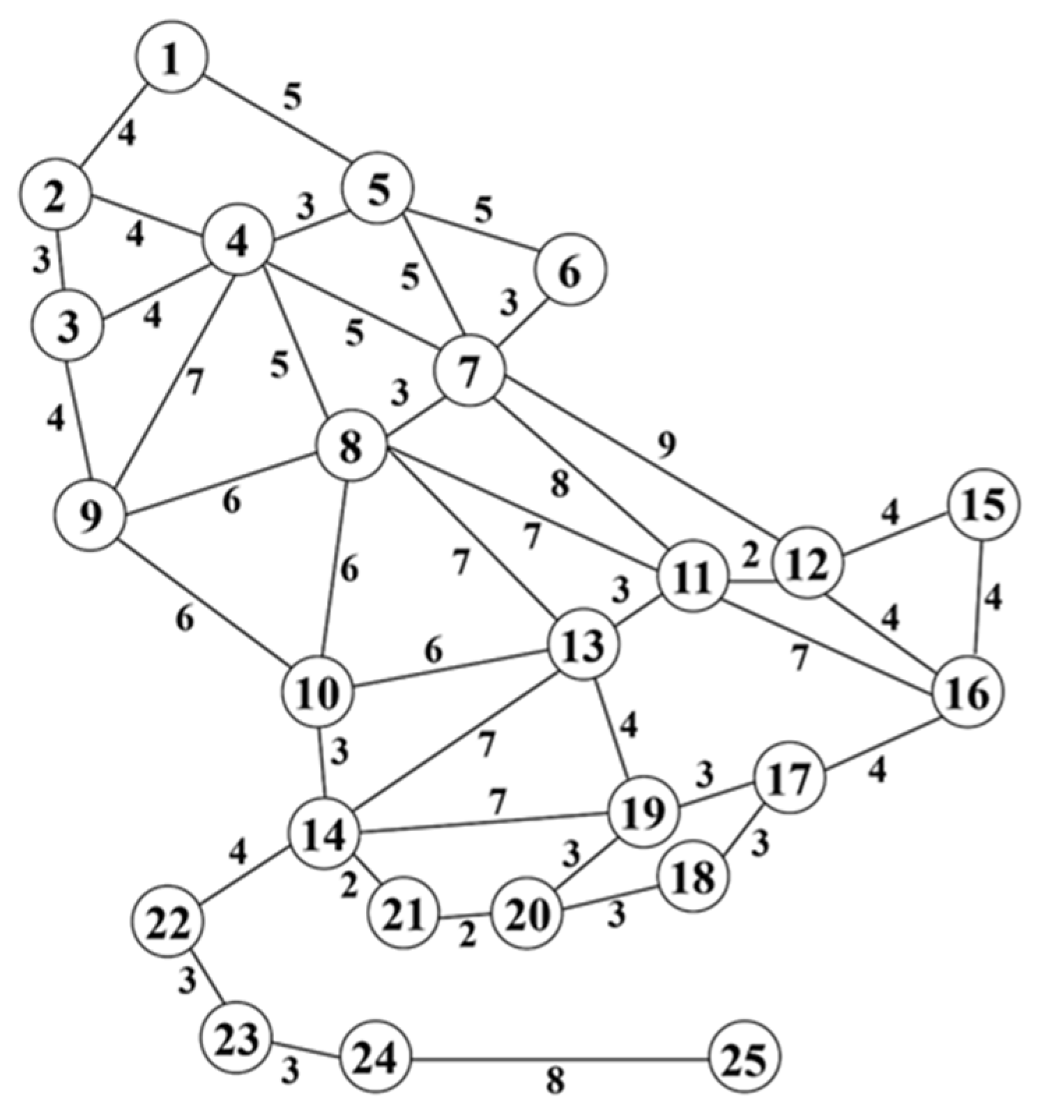
5.1. Example Description

In this paper, an example analysis is carried out by using the benchmark 25-node traffic network to verify the effectiveness of the model, and the results are compared and analyzed. The benchmark 25-node traffic network is a hypothetical network consisting of 25 nodes and 86 links (43 road sections), as shown in Figure 4.

This network has been applied to the research of electric vehicle charging station location optimization by many experts and scholars, such as Hodgson [2], Kuby [3,4,5], and Berman et al. [20]. The length of the road section and the importance of the nodes in the network use the data of Berman. At the same time, the length of the road section is also the range consumption of the electric vehicle driving through the road section, and the unit length represents 30 km. All of the nodes in the network can be used as the starting point, destination, and candidate location of the charging station. There are 300 OD pairs and 25 candidate locations of the charging station. The gravity model is used to estimate the traffic flow of each OD pair of electric vehicles, as shown in Equation (24):

$$f^q=O{D}_{ij}=\frac{W_i{W}_j}{l_{ij}{}^{1.5}}$$

(24)

where f^q and OD_ij are the traffic flow between node i and node j, where the single subscript q corresponds to the double subscript i,j, and W_i and W_j are the weights of node i and node j, respectively.

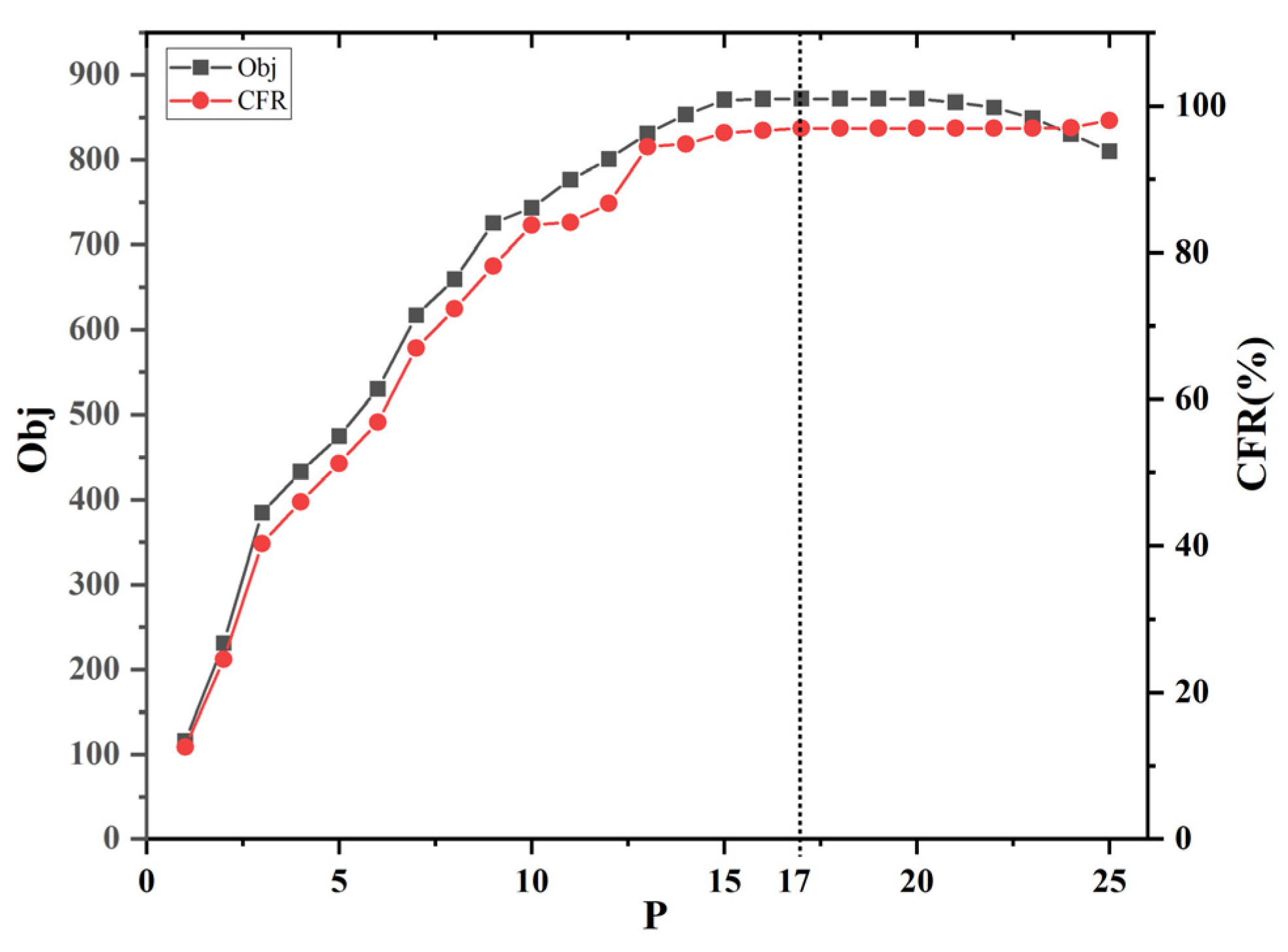
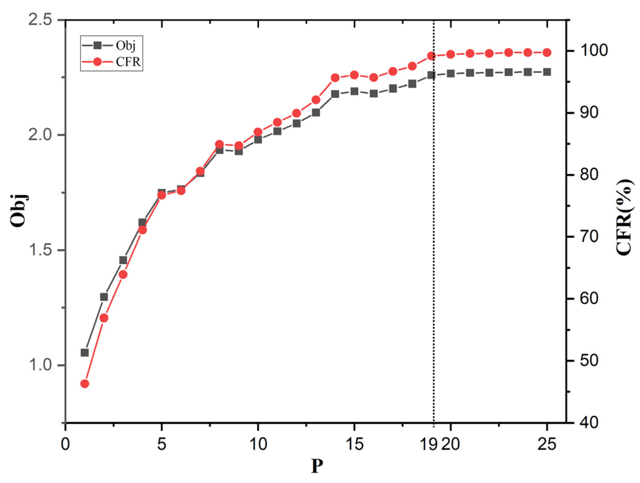
5.2. Solution Result

In this paper, the Tabu search algorithm was used to solve the model. Setting the weight ratio of the two sub-objective functions in the model, taking ${\omega }_1:{\omega }_2=7:1$ as an example, and assuming the range DR = 240 km of the electric vehicle in the model, the number of charging stations to be built $P=1,2,3,\cdots ,25$ for the electric vehicle, and the other parameters were all determined using the values in the reference [14]. The Tabu search algorithm was used to solve the above cases in turn, and the number of iterations was 500,000. The results are shown in

Table 2. Results of the model.

P	Obj	CFR (%)	Location Result
1	116.25	12.59	20
2	231.38	24.55	14,23
3	384.50	40.29	14,18,23
4	433.00	46.04	14,18,22,23
5	475.00	51.26	14,16,18,22,23
6	530.13	56.92	4,8,10,14,18,23
7	616.88	67.00	4,8,10,18,21,22,24
8	659.75	72.30	4,8,10,16,18,21,22,24
9	725.38	78.15	3,4,8,9,10,18,21,22,24
10	743.38	83.72	2,4,8,9,10,16,18,21,22,23
11	776.88	84.08	3,4,8,9,10,15,16,18,21,22,23
12	801.00	86.69	3,4,8,9,10,11,15,16,18,21,22,23
13	831.25	94.42	3,4,8,9,10,11,13,14,16,17,20,22,24
14	853.50	94.78	3,4,8,9,10,11,13,14,16,18,19,21,22,23
15	870.88	96.31	3,4,8,9,10,11,13,14,15,16,18,19,21,22,23
16	871.88	96.67	3,4,7,8,9,10,11,13,14,15,16,18,19,20,22,23
17	872.00	96.94	1,3,4,7,8,9,10,11,13,14,15,16,18,19,20,22,23
18	872.00	96.94	1,3,4,6,7,8,9,10,11,13,14,15,16,18,19,21,22,23
19	872.00	96.94	1,3,4,6,7,8,9,10,11,13,14,15,16,18,19,21,22,23,24
20	872.00	96.94	1,3,4,6,7,8,9,10,11,13,14,15,16,18,19,21,22,23,24,25
21	868.20	96.94	1,2,3,4,6,7,8,9,10,11,13,14,15,16,18,19,21,22,23,24,25
22	862.00	96.94	1,2,3,4,6,7,8,9,10,11,12,13,14,15,16,18,19,21,22,23,24,25
23	849.50	96.94	1,2,3,4,6,7,8,9,10,11,12,13,14,15,16,18,19,20,21,22,23,24,25
24	830.40	97.03	1,2,3,4,5,6,7,8,9,10,11,12,13,14,15,16,18,19,20,21,22,23,24,25
25	810.00	98.02	1,2,3,4,5,6,7,8,9,10,11,12,13,14,15,16,17,18,19,20,21,22,23,24,25

. The feasible path flow ratio (CFR) is the percentage of the feasible path flow in the total flow in the road network.

The distribution of the results of the model is shown in Figure 5.

The proportion of feasible road flow (CFR) increases with the increase in the number of charging stations. When the number of charging stations reaches 25, the proportion of feasible road flow reaches the maximum value of 98.02%. The CFR cannot reach 100% because the range of electric vehicles is limited, and some roads exceed the range of electric vehicles, making them impassable even when they are fully charged. For example, the length of road section 7–12 is 270 km, but the range of electric vehicles is only 240 km, so the path through this section is not feasible, and even if all nodes set up charging stations, they cannot intercept all of the flow. At the same time, this reflects how in the site selection planning of charging stations, only considering the construction of charging stations at the nodes will result in that part of the path flow not being interceptable because of the limited range, so we should consider adding candidate positions of charging stations in the middle of long road sections to ensure that the distance between charging stations is less than the range of the electric vehicles, so that the electric vehicles can travel smoothly. Another way to solve this problem is to develop the battery technology of electric vehicles to improve their range.

With the increase in the number of charging stations, the objective function value Obj first increases and then decreases, reaching the maximum value of 872 when the number of charging stations is 17–20, and the reasonable number of charging stations in this node network is 17. This shows that in the transportation network, more charging stations are not necessarily better. There are many reasons for this, one of which is that when a large number of charging stations are built, drivers will choose to charge ahead of time in order to avoid range anxiety, which leads to more range anxiety. The problem of “charging ahead of time” can be explained by a simple example, as shown in Figure 6.

In this path, node i and node j are candidate positions of charging stations. When the number of charging stations to be built is one, assuming that the charging station is built at node i or j, the driver chooses to charge in order to avoid range anxiety, and the flow in this path can be intercepted. At this time, it can be seen that when node j establishes the charging station, the driver’s range anxiety is reduced, so node j is the better location result. However, when the number of charging stations to be built is two, both node i and node j set up charging stations, and the flow of the path can still be intercepted, but the model cannot tell which range anxiety of the two nodes is less. In order to avoid range anxiety, drivers choose to charge at node i in advance, and so they may not charge at node j, resulting in greater range anxiety. Because drivers will avoid risk from their own point of view, the increase in the number of charging stations will not necessarily make the solution of the model better, but the limitations of individual choice will lead to greater range anxiety. In addition, increasing the number of charging stations will also result in unnecessary construction and operating costs.

5.3. Comparative Analysis of Results

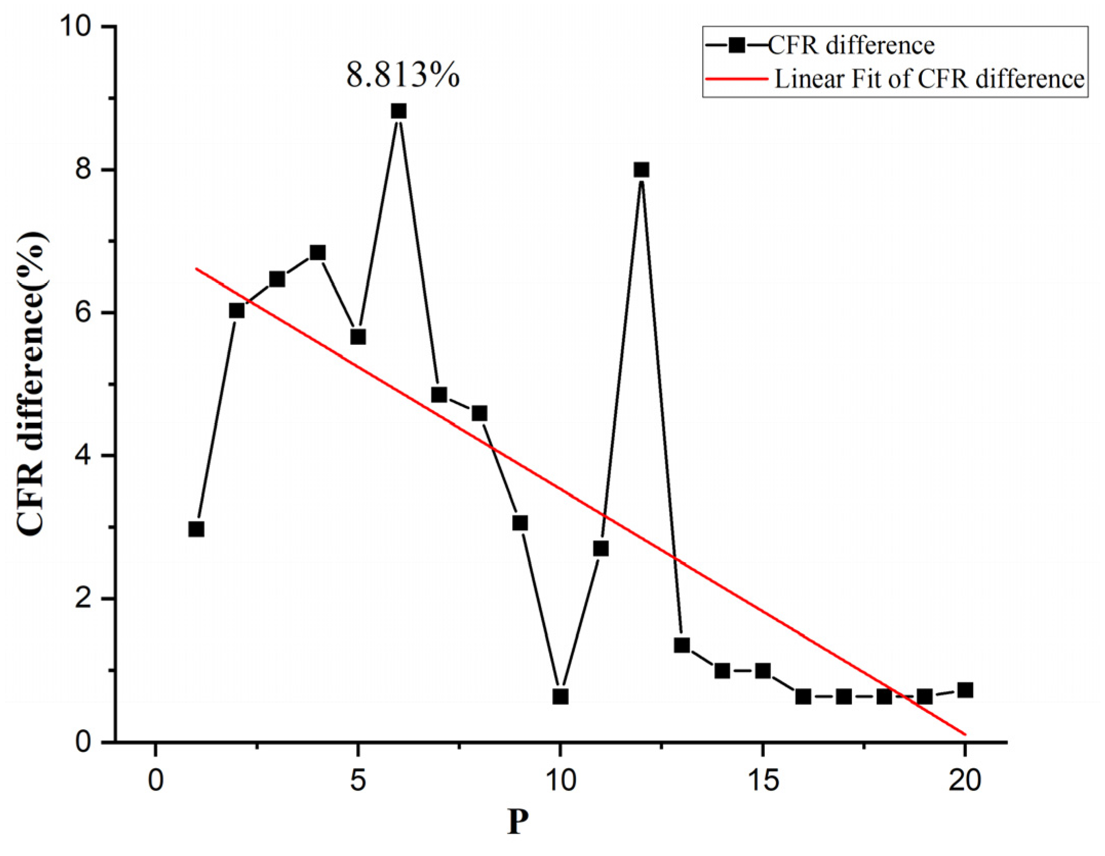
5.3.1. The Influence of Drivers’ Range Anxiety on Location Selection

In order to verify the effectiveness of considering the driver’s range anxiety in the electric vehicle charging station location planning, this paper makes the following experimental comparison: in the 25-node network, under the same parameter settings, the results of our model (hereafter referred to as model 1) and the maximum flow model are compared and analyzed. The electric vehicle range parameter is set to DR = 240 km. Because the reasonable number of 25-node network charging stations is P = 17, the increase in the number of charging stations will lead to a significant increase in solution time, and the number of electric vehicle charging stations to be built is set to $P\in \left.\left\{1,2,3,\cdots ,20\right.\right\}$.

The results are shown in

Table 3. Comparative analysis of the location results of model 1 and maximum flow model.

P	Obj	CFR (%)	Model 1 Location Result	P	Obj*	CFR (%)	Location Result of the Maximum Flow Model	Number of Location Differences
1	116.3	12.59	20	1	116.3	12.59	20	0
2	231.4	24.55	14,23	2	231.4	24.55	14,23	0
3	384.5	40.29	14,18,23	3	384.5	40.29	14,18,23	0
4	433.0	46.04	14,18,22,23	4	430.5	46.04	14,18,22,24	1
5	475.0	51.26	14,16,18,22,23	5	472.5	51.26	14,16,18,22,24	1
6	530.1	56.92	4,8,10,14,18,23	6	530.1	56.92	4,8,10,14,18,23	0
7	616.9	67.00	4,8,10,18,21,22,24	7	616.9	67.00	4,8,10,18,21,22,24	0
8	659.8	72.30	4,8,10,16,18,21,22,24	8	659.8	72.30	4,8,10,16,18,21,22,24	0
9	725.4	78.15	3,4,8,9,10,18,21,22,24	9	725.4	78.15	3,4,8,9,10,18,21,22,24	0
10	743.4	83.72	2,4,8,9,10,16,18,21,22,23	10	743.4	83.72	2,4,8,9,10,16,18,21,22,23	0
11	776.9	84.08	3,4,8,9,10,15,16,18,21,22,23	11	764.9	86.06	2,4,8,9,10,11,16,18,21,22,23	2
12	801	86.69	3,4,8,9,10,11,15,16,18,21,22,23	12	762.1	90.02	2,4,8,9,10,12,13,14,17,20, 22,24	7
13	831.3	94.42	3,4,8,9,10,11,13,14,16,17,20,22, 24	13	801.4	94.69	2,4,8,9,10,11,13,14,16,17, 20,22,24	1
14	853.5	94.78	3,4,8,9,10,11,13,14,16,18,19,21, 22,23	14	803.3	96.04	2,4,8,9,10,11,13,14,16,17, 19,20,22,23	3
15	870.9	96.31	3,4,8,9,10,11,13,14,15,16,18,19, 21,22, 23	15	814.4	97.57	3,4,8,9,10,11,13,14,15,16, 17,19,20,22,23	2
16	871.9	96.67	3,4,7,8,9,10,11,13,14,15,16,18, 19,20, 22,23	16	849.0	97.66	3,4,7,8,9,10,11,13,14,15,16, 17,19, 20,22,23	1
17	872.0	96.94	1,3,4,7,8,9,10,11,13,14,15,16,18, 19,20, 22,23	17	801.3	98.02	2,4,5,7,8,9,10,11,13,14,15, 16,17,19,20,22,23	3
18	872.0	96.94	1,3,4,6,7,8,9,10,11,13,14,15,16, 18,19, 21,22,23	18	808.8	98.02	1,2,4,5,7,8,9,10,11,13,14,15, 16,17, 19,20,22,24	5
19	872.0	96.94	1,3,4,6,7,8,9,10,11,13,14,15,16, 18,19, 21,22,23,24	19	796.3	98.02	2,4,5,7,8,9,10,11,13,14,15, 16,17,19,20,22,23,24,25	5
20	872.0	96.94	1,3,4,6,7,8,9,10,11,13,14,15,16, 18,19, 21,22,23,24,25	20	842.5	98.02	1,3,4,5,7,8,9,10,11,13,14,15, 16,17, 18,19,21,22,23,25	2

Remark: add * to the Obj of the maximum flow model to distinguish it from model 1.

. The results of the two models are listed in the table, the range anxiety of the driver in the maximum flow model is calculated, and the Obj* value of the maximum flow model is calculated according to the meaning and the weight ratio of Obj in model 1, which is used as an evaluation index for the comparison of the two results. At the same time, the table also lists the numbers of location differences generated by the two models.

As can be seen from Table 3, the two models can intercept the same traffic when the number of charging stations is 1–10; that is, they cover the same travel demand. However, when the number of charging stations is 4 or 5, different location results are produced. Among them, model 1 gives a more reasonable station distribution, which not only covers the same traffic, but also reduces the driver’s range anxiety. When the number of sites is 4 or 5, model 1 selects node 23 as the charging station location, while the maximum flow model selects node 24 as the charging station location. Both node 23 and node 24 can intercept the same traffic; that is, in the maximum traffic model, the choice of node 23 or node 24 can be used as the optimal solution, and the difference between the two nodes cannot be identified in the maximum traffic model. However, model 1 takes into account the driver’s range anxiety, so when selecting node 23 to build a charging station, the driver’s range anxiety is less than it is for node 24; that is, model 1 can identify the difference between the two nodes, and select node 23 as the better solution.

When the number of charging stations is from 1 to 20, the results of the two models are different. Between them, the biggest difference is that the number of charging stations built is 12, and the number of location differences between the two models is 7. The reasons are as follows: First of all, the maximum flow model cannot identify the driver’s range anxiety, and the optimal solution is obtained when the intercepted traffic is at its maximum, so there may be multiple optimal solutions obtained by the flow model, as shown in

Table 4. Obtaining multiple optimal solution examples with the maximum flow model.

P	Obj*	CFR (%)	Location Result of the Maximum Flow Model	Number of Location Differences
16	849.00	97.66	3,4,7,8,9,10,11,13,14,15,16,17,19,20,22,23	1
	809.00	97.66	2,4,6,8,9,10,11,13,14,15,16,17,19,20,22,24	4
18	808.75	98.02	1,2,4,5,7,8,9,10,11,13,14,15,16,17,19,20,22,24	5
	788.75	98.02	2,4,5,6,7,8,9,10,11,13,14,15,16,17,19,20,22,24	5
20	842.50	98.02	1,3,4,5,7,8,9,10,11,13,14,15,16,17,18,19,21,22,23,25	2
	806.25	98.02	2,3,4,5,6,7,8,9,10,11,12,13,14,15,16,17,19,20,22,23	5

Remark: add * to the Obj of the maximum flow model to distinguish it from model 1.

. Secondly, when there are a large number of charging stations, due to the setting of the weight ratio and other parameters, the driver’s range anxiety is greater, which will have an impact on the final result, resulting in the intercepted flow being slightly lower than that of the maximum flow model. As a result, the results will be different. Adjusting the weight ratio and increasing the weight of intercepted traffic can reduce the difference between the two models.

The ratio of Obj difference (the ratio of the difference in Obj between the two models to the Obj of model 1) and the ratio of CFR difference (the ratio of the difference in CFR between the two models to the maximum flow model’s CFR) were compared with the number of charging stations built, as shown in Figure 7. It can be seen that except for the proportion of CFR difference being higher than that of Obj difference when the number of charging stations is 11, in other cases, the proportion of Obj difference is higher than that of CFR difference. This shows that the degree of reduction in traffic interception caused by range anxiety in model 1 is less than that in the maximum flow model, which only considers the increase in range anxiety. At the same time, it shows that when the weight ratio is a large value, model 1 and the maximum flow model can intercept the same traffic, but in the solution of model 1, the driver has less range anxiety and the location result is better. The above effect can be achieved when the weight ratio is 100:1.

In summary, the maximum interception flow is the best in the traditional FCLM, but when the interception flow is maximum, there may be multiple optimal solutions, while the dual-objective location model established in this paper can select the solution with the least range anxiety among the multiple optimal solutions, and then find a better solution.

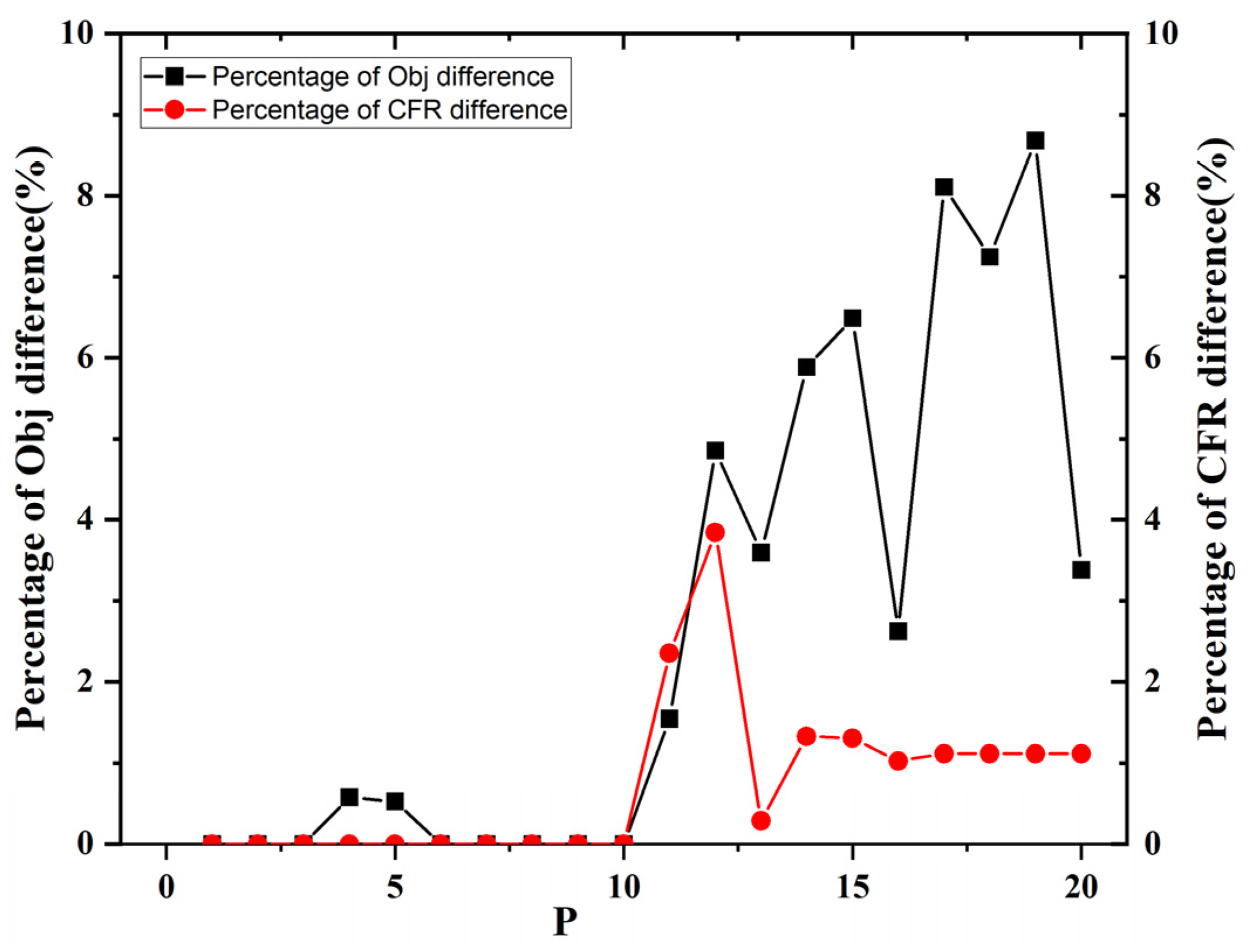
5.3.2. The Influence of Charging Selection Behavior on Location Selection

In order to analyze the influence of the driver’s charging selection behavior on the charging station location, the constraints (14) and (15) in model 1 are omitted, and it is assumed that $y_i^q=1$; that is, the driver must charge when they arrive at the charging station. This can be simplified to a dual-objective model without considering charging selection, which is referred to as model 2. This paper makes the following experimental comparison: based on the 25-node traffic network, under the same parameter settings, model 1 and model 2 are solved, and the results are compared and analyzed. The electric vehicle range parameter is set to DR = 240 km, and the number of electric vehicle charging stations to be built is $P\in \left.\left\{1,2,3,\cdots ,20\right.\right\}$, λ = 1.

The results are shown in

Table 5. Comparative analysis of the location results of model 1 and model 2.

P	CFR (%)	Charging Times	Model 1 Location Result	P	CFR (%)	Charging Times	Model 2 Location Result
1	12.59	9	20	1	15.56	11	14
2	24.55	29	14,23	2	30.58	24	14,18
3	40.29	54	14,18,23	3	46.76	69	14,18,23
4	46.04	65	14,18,22,23	4	52.88	103	14,16,18,23
5	51.26	95	14,16,18,22,23	5	56.92	109	4,14,16,18,23
6	56.92	199	4,8,10,14,18,23	6	65.74	278	4,8,10,14,18,23
7	67.00	251	4,8,10,18,21,22,24	7	71.85	312	4,8,10,14,16,18,23
8	72.30	292	4,8,10,16,18,21,22,24	8	76.89	435	3,4,8,9,10,14,18,23
9	78.15	382	3,4,8,9,10,18,21,22,24	9	81.21	502	3,4,8,9,10,14,17,20,23
10	83.72	499	2,4,8,9,10,16,18,21,22,23	10	84.35	487	3,4,8,9,10,16,18,21,22,23
11	84.08	436	3,4,8,9,10,15,16,18,21,22,23	11	86.78	529	3,4,8,9,10,11,16,18,21,22,23
12	86.69	487	3,4,8,9,10,11,15,16,18,21,22,23	12	94.69	777	3,4,8,9,10,11,13,14,16,17,20,23
13	94.42	615	3,4,8,9,10,11,13,14,16,17,20,22, 24	13	95.77	836	3,4,8,9,10,11,13,14,16,17,19, 20,23
14	94.78	677	3,4,8,9,10,11,13,14,16,18,19,21, 22,23	14	95.77	926	3,4,8,9,10,11,13,14,16,17,19, 20,22,23
15	96.31	720	3,4,8,9,10,11,13,14,15,16,18,19, 21,22,23	15	97.30	975	3,4,8,9,10,11,13,14,15,16,17, 19,20,22,23
16	96.67	782	3,4,7,8,9,10,11,13,14,15,16,18,19, 20,22,23	16	97.30	1011	3,4,8,9,10,11,12,13,14,15,16, 17,19,20,22,23
17	96.94	843	1,3,4,7,8,9,10,11,13,14,15,16,18, 19,20,22, 23	17	97.57	1065	1,2,3,4,8,9,10,11,13,14,15,16, 17,19,20,22, 24
18	96.94	850	1,3,4,6,7,8,9,10,11,13,14,15,16, 18,19,21,22, 23	18	97.57	1101	1,2,3,4,8,9,10,11,12,13,14,15, 16,17,19,20, 22,24
19	96.94	838	1,3,4,6,7,8,9,10,11,13,14,15,16, 18,19,21,22, 23,24	19	97.57	1158	1,2,3,4,8,9,10,11,12,13,14,15, 16,17,18,19, 21,22,24
20	96.94	838	1,3,4,6,7,8,9,10,11,13,14,15,16, 18,19,21,22, 23,24,25	20	97.66	1237	1,2,3,4,5,6,8,9,10,11,12,13,14, 15,16,17,19, 20,22,23

, which lists the results of the two models, and calculates the charging times of the driver along the feasible path, which is used as an evaluation index for the comparison of the two results. The results show that the CFR of model 1 is smaller than that of model 2, because the driver’s charging choice behavior is considered in model 1, and the driver often charges in advance due to range anxiety, resulting in subsequent travel failure, or the driver chooses not to charge, resulting in travel failure, so the intercepted traffic in model 1 is small. However, because considering the driver’s charging choice is more in line with the actual travel situation, the solution is more scientific and reasonable. The result of model 2 assumes that the driver must recharge when they arrive at the charging station, so the CFR of the solution is higher, but the result is not consistent with the actual situation, and will lead to the wrong location choice for planning decision makers. In addition, with the increase of the number of charging stations, the CFR difference between the two models tends to decrease, as shown in Figure 8.

Because model 2 assumes that the driver must be recharged when they arrive at the charging station, it will result in more charging instances than model 1, as shown in Figure 9. With the increase in the number of charging stations, the difference between the numbers of charging instances of the two models increases. When the number of charging stations is 20, the difference between the charging instances of the two models reaches the maximum of 399 times. The huge difference in the number of instances of charging first means huge charging costs and operating costs, including the driver’s charging costs and time costs. Taking the reasonable construction number of 17 charging stations as an example, the difference between the numbers of charging instances of the two models is 222, and the difference in feasible path flow is 6. It is preliminarily estimated that the average cost of each charge of an electric vehicle is CNY 146.4, and the average penalty cost per unit of travel is CNY 922.4. Compared with model 2, model 1 saves CNY 32,500.8 in charging costs and a further CNY 5534.4 in penalty costs; that is, model 1 saves CNY 26,966.4 compared with model 2.

5.4. Empirical Analysis

In order to test the effectiveness of the model and algorithm in practical application, this paper uses the expressway network of Jilin Province for empirical analysis. The network is simplified by Jilin expressway, which is composed of 62 nodes and 75 road sections, each of which is bidirectional. Thirty-seven expressway service areas are selected as candidate locations for charging stations.

Assuming that the range of the electric vehicle in the expressway network of Jilin Province is DR = 240 km, the number of charging stations to be built is $P\in \left.\left\{1,2,3,\cdots ,25\right.\right\}$, the weight ratio is set to ${\omega }_1:{\omega }_2=9:1$, and the other parameters follow the value of the 25-node traffic network example. The Tabu search algorithm is used to solve the problem, and the number of iterations is 1 million. The results are shown in

Table 6. Results for the expressway network in Jilin Province.

P	Obj	CFR (%)	Location Result
1	1.0547	46.29	8
2	1.2960	56.89	8,10
3	1.4563	63.92	8,10,12
4	1.6196	71.08	8,10,14,16
5	1.7482	76.71	5,8,10,14,16
6	1.7645	77.45	4,8,10,14,15,16
7	1.8356	80.60	3,8,10,14,16,22,53
8	1.9338	84.92	8,10,14,16,22,24,35,53
9	1.9297	84.70	8,10,14,16,19,22,35,43,47
10	1.9797	86.90	4,5,8,9,10,12,14,16,53,54
11	2.0161	88.48	5,8,10,14,16,21,36,40,47,53,60
12	2.0503	89.94	5,8,10,11,12,14,16,20,22,29,43,54
13	2.0978	92.10	6,8,10,14,15,16,20,22,30,35,37,45,54
14	2.1782	95.63	6,8,10,14,15,16,20,22,25,30,35,40,54,58
15	2.1904	96.08	2,4,5,6,8,10,12,14,15,16,20,22,24,27,58
16	2.1804	95.69	4,5,8,10,11,14,15,16,22,26,35,39,52,56,57,61
17	2.2018	96.67	5,6,8,10,12,14,16,18,25,27,28,40,48,53,56,58,61
18	2.2225	97.51	3,4,7,8,10,14,15,16,19,22,24,26,35,45,52,55,56,61
19	2.2594	99.17	3,4,5,8,10,11,13,14,15,16,20,22,24,26,27,30,35,45,56
20	2.2667	99.42	3,4,5,6,8,10,12,14,15,16,18,21,24,26,27,44,53,55,59,61
21	2.2694	99.56	1,4,5,6,7,9,12,14,15,16,20,22,23,24,27,33,36,38,40,56,57
22	2.2697	99.58	2,3,4,5,6,7,8,9,12,13,14,15,16,18,19,23,26,34,35,53,56,62
23	2.2725	99.73	4,5,8,10,14,15,16,17,19,20,21,23,26,27,37,38,43,45,51,55,56,57,60
24	2.2727	99.73	2,5,6,7,8,9,10,14,15,16,18,20,23,26,31,33,40,45,46,48,52,56,57,62
25	2.2736	99.73	2,4,5,6,8,10,11,12,15,16,18,19,20,21,23,24,26,32,44,48,55,56,57,60,62

Remark: The optimal charging station construction scheme is highlighted in bold.

.

When plotting the data in Table 6 as shown in Figure 10, it can be seen that when the number of charging stations is 19, the proportion of feasible path traffic to CFR reaches 99.17%, which can intercept the vast majority of traffic in the network. When the number of charging stations is higher than 19, the ratio of objective function value and feasible path flow increases at an extremely slow rate—almost horizontally. Therefore, in the expressway network of Jilin Province, the planning and construction of 19 charging stations is more reasonable. The construction distribution of charging stations is shown in Figure 11.

6. Conclusions

Based on the analysis of drivers’ charging choice behavior and range anxiety, this paper studied the location of charging stations in an expressway network under the limited conditions of the number of charging stations. First of all, the relationship between the driver’s charging selection behavior, range anxiety, and charging station location was analyzed, and the necessity of considering them in the charging station location model was introduced. The path feasibility analysis was carried out on the basis of the FRLM, and the FRLM was improved to avoid the pre-generation of charging facilities in the FRLM and make the model more compact. Based on this, a dual-objective charging station location model with maximal flow capture and minimal driver range anxiety was constructed, and the model was extended by adding candidate positions of charging stations along the road section. A heuristic algorithm—the Tabu search algorithm—was proposed to solve the model. Then, a 25-node traffic network was used to analyze the example, the Tabu search algorithm was used to solve the model, and a random scene was selected to verify and analyze the algorithm. The results of the model were compared and analyzed, and the results showed that the charging station location model considering drivers’ charging choice behavior and range anxiety performs better. Finally, the Jilin expressway network was used for empirical analysis, to verify the effectiveness of the model and algorithm in practical application, and to obtain the schematic diagram of the Jilin expressway network’s charging station layout.

The method proposed in this paper can provide government departments with a preliminary location scheme for the construction of electric vehicle charging stations on expressway networks or national highway networks. This paper also has a certain reference significance for the location of electric vehicle charging stations, but there are still limitations. Further research will be carried out on the following aspects in the future: First, in this paper, the capacity of charging stations was not considered in the problem hypothesis. Considering the fixed capacity of the charging station in the location of the charging station needs to be further studied. Second, this paper only considers the feasibility of the electric vehicle in the path, assuming that the driver goes to the destination along the shortest path. However, in fact, drivers will deviate from their original driving path because of the need for charging, and the problem considering this factor is collectively referred to as the offset path problem. In the next step, the model should be extended in the direction of the offset path, and the feasibility of electric vehicles in the network should be studied.

References

1. Egbue, O.; Long, S. Barriers to widespread adoption of electric vehicles: An analysis of consumer attitudes and perceptions. Energy Policy 2012, 48, 717–729. [Google Scholar] [CrossRef]
2. Hodgson, M. A flow-capturing location—Allocation model. Geogr. Anal. 1990, 22, 270–279. [Google Scholar] [CrossRef]
3. Kuby, M.; Lim, S. The flow-refueling location problem for alternative-fuel vehicles. Soc.–Econ. Plan. Sci. 2005, 39, 125–145. [Google Scholar] [CrossRef]
4. Kuby, M.; Lim, S. Location of alternative-fuel stations using the flow-refueling location model and dispersion of candidate sites on arcs. Netw. Spat. Econ. 2007, 7, 129–152. [Google Scholar] [CrossRef]
5. Kim, J.; Kuby, M. The deviation-flow refueling location model for optimizing a network of refueling stations. Int. J. Hydrog. Energy 2012, 37, 5406–5420. [Google Scholar] [CrossRef]
6. Guo, F.; Yang, J.; Lu, J. The battery charging station location problem: Impact of users’ range anxiety and distance convenience. Transp. Res. Part E-Logist. Transp. Rev. 2018, 114, 1–18. [Google Scholar] [CrossRef]
7. Chung, S.H.; Kwon, C. Multi-period planning for electric car charging station locations: A case of Korean Expressways. Eur. J. Oper. Res. 2015, 242, 677–687. [Google Scholar] [CrossRef]
8. Capar, I.; Kuby, M.; Leon, V.J.; Tsai, Y.J. An arc cover-path-cover formulation and strategic analysis of alternative-fuel station locations. Eur. J. Oper. Res. 2013, 227, 142–151. [Google Scholar] [CrossRef]
9. Xu, M.; Yang, H.; Wang, S. Mitigate the range anxiety: Siting battery charging stations for electric vehicle drivers. Transp. Res. Part C-Emerg. Technol. 2020, 114, 164–188. [Google Scholar] [CrossRef]
10. Zhu, Z. Charging Station Location Problem of Electric Vehicles. Ph.D. Thesis, Beijing Jiaotong University, Beijing, China, 2018. [Google Scholar]
11. Gao, S.; Frejinger, E.; Ben-Akiva, M. Adaptive route choices in risky traffic networks: A prospect theory approach. Transp. Res. Part C-Emerg. Technol. 2010, 18, 727–740. [Google Scholar] [CrossRef]
12. Schwanen, T.; Ettema, D. Coping with unreliable transportation when collecting children: Examining parents’ behavior with cumulative prospect theory. Transp. Res. Part A-Policy Pract. 2009, 43, 511–525. [Google Scholar] [CrossRef]
13. Xu, H.; Zhou, J.; Xu, W. A decision-making rule for modeling travelers’ route choice behavior based on cumulative prospect theory. Transp. Res. Part C-Emerg. Technol. 2011, 19, 218–228. [Google Scholar] [CrossRef]
14. Hu, L.; Dong, J.; Lin, Z. Modeling charging behavior of battery electric vehicle drivers: A cumulative prospect theory based approach. Transp. Res. Part C-Emerg. Technol. 2019, 102, 474–489. [Google Scholar] [CrossRef] [Green Version]
15. Zhang, J. Modeling and Analyzing of Driving Mileage of Electric Vehicle Based on Data-driven. Master’s Thesis, Beijing Jiaotong University, Beijing, China, 2015. [Google Scholar]
16. Xu, M.; Meng, Q.; Liu, K.; Yamamoto, T. Joint charging mode and location choice model for battery electric vehicle users. Transp. Res. Part B-Methodol. 2017, 103, 68–86. [Google Scholar] [CrossRef]
17. Yang, Y.; Yao, E.; Yang, Z.; Zhang, R. Modeling the charging and route choice behavior of BEV drivers. Transp. Res. Part C-Emerg. Technol. 2016, 65, 190–204. [Google Scholar] [CrossRef]
18. Franke, T.; Neumann, I.; Buhler, F.; Cocron, P.; Krems, J.F. Experiencing Range in an Electric Vehicle: Understanding Psychological Barriers. Appl. Psychol.-Int. Rev.-Psychol. Appl.-Rev. Int. 2012, 61, 368–391. [Google Scholar] [CrossRef]
19. Wang, Y.; Lin, C. Locating road-vehicle refueling stations. Transp. Res. Part E-Logist. Transp. Rev. 2009, 45, 821–829. [Google Scholar] [CrossRef]
20. David, S.; Oded, B. A Heuristic Algorithm for the Traveling Salesman Location Problem on Networks. Oper. Res. 1988, 36, 377–513. [Google Scholar]
Figure 1. Schematic diagram of the range anxiety power function.
Sustainability 14 04213 g001
Figure 2. Example diagram of the charging logic of an electric vehicle in a linear path.
Sustainability 14 04213 g002
Figure 3. Example diagram of the charging logic of an electric vehicle in a linear path.
Sustainability 14 04213 g003
Figure 4. A hypothetical 25-node network.
Sustainability 14 04213 g004
Figure 5. Results of the model ( ω 1 : ω 2 = 7 : 1 ).
Sustainability 14 04213 g005
Figure 6. Schematic diagram of a driver’s “charging in advance”.
Sustainability 14 04213 g006
Figure 7. The proportion diagram of the difference between model 1 and the maximum flow model.
Sustainability 14 04213 g007
Figure 8. The CFR difference distribution map of the results of model 1 and model 2.
Sustainability 14 04213 g008
Figure 9. The difference in the number of charging instances between model 1 and model 2.
Sustainability 14 04213 g009
Figure 10. Results for the expressway network in Jilin Province.
Sustainability 14 04213 g010
Figure 11. Schematic diagram of the network charging station layout of the expressway in Jilin Province.
Sustainability 14 04213 g011