Research on the Division Method of Signal Control Sub-Region Based on Macroscopic Fundamental Diagram

Abstract

The macroscopic fundamental diagram (MFD) provides a method to evaluate macro traffic operation through micro traffic parameters, which can be applied to traffic control to prevent traffic congestion transfer and improve road network efficiency. However, due to the large scale of the urban road network as well as the complex temporal and spatial distribution of road congestion, the application of the MFD for signal control first requires the partition of the urban road network. Based on the analysis of MFD partition purposes, a set of MFD partition methods based on graph theory was designed. Firstly, graph theory was used to transform the urban road network; secondly, the minimum spanning tree method was used to divide the urban traffic network map. Moreover, the attribution of the link between connected regions is determined. Our method can solve the problem of ambiguous intersection ownership, and the road sections belonging to the same road in opposite directions are separated. This method has the ability to control the size of the area by limiting the number of intersections; Finally, the evaluation index of regional clustering results was drawn. To achieve the research objective, we collected and processed vehicle information data from the Xuzhou car-hailing platform to obtain traffic density information. Then, we selected an area with sufficient data and a large enough road network. The empirical value range of the regional control value was obtained by comparing the values of multiple groups of measurement data k and evaluation indexes. In this process, it was found that during the period of flat peak and peak transition, while the regional average traffic density changes, the uniformity of traffic density first decreases and then increases. The traffic density uniformity of the signal control area can be improved by controlling the size of the signal control area. We obtained the empirical value range of the regional control value k by comparing the values of multiple groups of measurement data k and evaluation indexes. Then, we compared them with the two kinds of traditional partition algorithms and improved multiple dichotomy algorithms. Our method improves road network balance by 5% over existing methods.

1. Introduction

Urban traffic problems have been troubling the development of the city. The contradiction between traffic demand and traffic land further aggravates urban traffic congestion. At present, the analysis and modeling of traffic congestion mainly relied on physics, fluid mechanics, queuing theory, and other ideas [1]. The fundamental diagram described the relationship between three elements of traffic, namely density, speed, and flow in a single road section, providing a clear partition of traffic states for most traffic theories. However, the above ideas all took local traffic as the research object and lack the description of the traffic system, which lead to frequent traffic congestion transfer in the management and control of traffic congestion.

In 2007, a study of Yokohama traffic statistics found that a well-defined macroscopic fundamental diagram (MFD) exists between urban traffic flow and average traffic density [2]. The following conclusions were drawn: (1) Urban communities exhibit a general “MFD” that relates the traffic flow to the average spatial speed (or flow). (2) There is a robust linear relationship between the average flow of the neighborhood and its total outflow. (3) The MFD is an attribute of road network infrastructure and signal control, instead of requirements; i.e., spatial average traffic is maximized for the same value of vehicle density independent of the time-dependent origin table [3,4]. The macroscopic fundamental diagram phases can be divided into four stages: smooth, congested, blocked, and congested dissipated. (Smooth: high vehicle speed, low traffic flow, and the vehicles running without interference from the preceding vehicle. Congested: low driving speed, high traffic flow, vehicle following. Blocked state: low driving speed, low traffic flow, vehicles approaching stagnation. Congestion Dissipation State: Traffic flow is low and traffic density gradually decreases). The state division of the macroscopic fundamental diagram is shown in Figure 1. It is seen that the MFD describes the operational status of the traffic. The signal control in targeted regions is based on the different regional traffic conditions described by MFD, which provides a theoretical basis for regional traffic control.

The subsequent empirical study found that the MFD has scattering properties, especially when the traffic density is uneven in the road network, the vertex of the MFD will be lower [5,6,7]. The analysis of traffic data for medium-sized cities in France shows that heterogeneity has a more substantial impact on the shape and scatter of the MFD [8]. Empirical evidence and simulation data demonstrate that the distribution of vehicle density in the network has a greater impact on the formation of the MFD [9,10]. Research also shows that the MFD is continuously changing with the traffic flow [11,12]. With the deepening of research, the MFD is found to have uncertainties, and these uncertainties can cause congestion [13]. A study of a region in South Korea found that average network traffic usually lags behind changes in density [14]. Moreover, the traffic density distribution affects the MFD [15,16]. And the boundary capacity also has an impact on the outflow of traffic flow [17].

Those above-mentioned MFD-based urban traffic management methods should be based on the identification of MFD areas. MFD partitioning is a typical spatial clustering problem. The spatial clustering methods mainly include the growth method and the segmentation method.

The principle of the growth method is to find a few essential points and then choose whether to absorb the energy by continuously comparing it with the adjacent elements. This method needs to have a specific prediction on the final cluster family, and then, we set the number and position of the initial base points. The K-means is a typical growth algorithm. In the case of a certain number of clusters, the intra-cluster population variance is minimized, and the clustering of high-similar density segments can be well generated. However, it is challenging to ensure the tightness of the entire space, and the result is highly dependent on the selection of the initial growth point [18]. Recently, clustering-based MFD region partitioning methods had emerged, but this method was oriented to large-scale transportation networks. The segmentation sub-regions in the segmentation results were extensive, which was not suitable for urban traffic management [19]. Mohammadreza and Geroliminis proposed a dynamic clustering method of urban traffic network based on the degree of congestion [20], and they further improved this method for MFD division by limiting the population length [21]. This method focuses on link cluster growth, which is helpful for travel time estimation but is disadvantageous for regional signal control. Lin proposed an MFD partition method based on the spectral clustering algorithm, which ignores the topological characteristics of the road network [22]. A.F and Lentzakis developed an MFD division method based on regional growth technology, which focuses on road segment clustering and fails to handle intersections well [23].

The idea of the segmentation method is to divide the whole region according to the similarities between clusters and the similarity within groups and divide the entire network into several parts according to specific standards, mainly including Minimum Cut and N-cut. The Minimum Cut target is the smallest similarity between clusters and is usually used to cut outliers, but in traffic networks, too many sub-partitions are not conducive to signal control management. N-cut adds a similarity requirement to the interior of the cluster based on the goal of Minimum Cut. Since the two partition targets have specific conflicts, the partition result can provide an excellent initial partition but does not produce the best product. If the threshold is too low, then the uniform area may be split into two. The cutting result of the method has the possibility of dividing sections of a road with different traffic directions into other clusters when applied to the urban road network, which is not conducive to the formulation and implementation of the later control measures [24]. Most of the MFD partition now uses an improved method based on the segmentation method and is usually supplemented by a merge process after division [25,26].

However, among the above division methods, some methods combine the sections of the same road that pass through in two directions. When two sections of the same route with different driving directions are considered separately, the two sections with varying directions of driving are often divided into different sub-zones, which is extremely unfavorable for the later regional signal control, so it is necessary to control the shape of the sub-area at the end of the division. Even if morphological control is carried out, the result of the division is the road section as the boundary, and the management of the boundary road section is still tricky.

The urban road network is composed of several roads with two-way traffic sections, and two different traffic directions of one route have different traffic densities. The essence of the partition of MFD is the spatial clustering of areas with different densities [27]. According to the characteristics of urban road composition and density distribution, the result of partitioning is likely to separate the two directions of a road, which is not conducive to regional signal control. Moreover, the area of urban coordination signal control should not be too large or too small, and the immense control area will lead to more control intersections, increasing the complexity of the control computing model and calculation time, which is not conducive to the implementation of real-time signal control. A small control area will lead to increasing partitioned regions and increase the difficulty of coordinated control between areas.

Therefore, in the partition of MFD, the considered points are (1) different directions and density characteristics of roads, (2) road integrity, (3) the stable spatial distribution of density values in each region, and (4) the absolute scale for the design of regional control. It is not easy to use the road segment as the object of partition. Moreover, the network partition result is more suitable for subsequent regional signal control with the intersection as the demarcation point. Therefore, the connection characteristics of intersections in the road network should be considered in the partition.

We propose a heterogeneous transportation network division method that divides the transportation network into clusters with small density differences. However, since most urban roads are composed of road sections with different directions, it was not conducive to implementing signal control to divide different driving directions of one route into other clusters. The partitioning method maintained the integrity of the road network while minimizing density differences between regions, and it used the intersection as a partition point to facilitate the implementation of the signal control [28,29,30].

Graph-based segmentation is mainly applied to image segmentation. It is a classic image segmentation algorithm, which is a graph-based elastic clustering algorithm [31]. It is easy to use, with fast processing speed and high accuracy. Many similar algorithms have emerged based on graph-based segmentation, such as Over Segmentation and Semantic Segmentation [32,33]. The urban transportation network consists of a large number of road sections and intersections. The essence of urban MFD partition is the spatial clustering problem of weighted road sections. The graph-based segmentation method firstly establishes an undirected connection graph with weighted targets and then decides whether to merge by analyzing the indexes of the connected targets.

The road network density of urban road traffic system is large, and the traffic density of adjacent sections is different. According to the macroscopic fundamental diagram theory, when the traffic density of regional road sections tends to be consistent, the traffic efficiency of the region is higher. Therefore, the signal control area with higher traffic efficiency can be obtained by dividing the road network based on the similar traffic density of the road sections. Based on macroscopic fundamental diagram, we develop a novel traffic signal control region partitioning method. This method describes the relationship between intersections and road segments through graph theory, takes the intersection as the division object, and judges the ownership of the intersection by comparing the vehicle density of the sections connected to the intersection.

This method is mainly applied to the signal control area division of urban road traffic system with a dense road network. Through this method, the boundary of the signal control area of the urban road system and the attribution of the signal intersection can be determined. This method can eliminate the problem that the intersection assignment of the final divided area is not clear and the opposite direction of the road is divided. At the same time, the method can effectively control the scale of the final divided area. This method can divide the road network into better signal control areas and support the implementation of signal control based on macroscopic fundamental diagram.

This article is organized as follows:

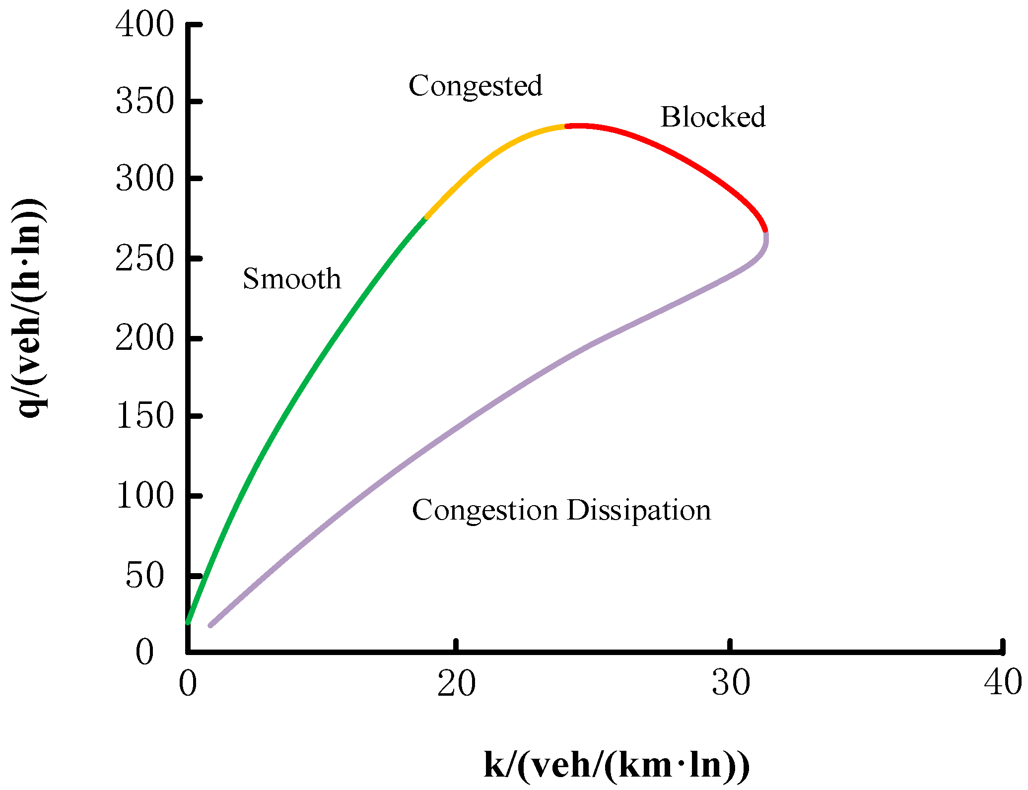
Methodology: The flow of the urban road network MFD partition method based on graph theory in detail was designed and described. The method is divided into three parts: 2.1 Urban Road Network Abstract Diagram, 2.2 Segmenting, and 2.3 Boundary determination;

Metrics development: The spatial metric is introduced to evaluate the clustering results;

Implement: This method is applied to a real transportation network to obtain the value range of regional control parameters and compare it with other clustering algorithms. It contains three parts: 4.1 Network and data description, 4.2 Result analysis and 4.3 Method comparison;

Conclusions and future development: The future research directions of regional partition are also introduced.

2. Methodology

According to the above analysis, the goal of this paper is to divide the urban road network into different clusters according to the density characteristics of the MFD. The partition results need to meet the following objectives: (1) the density distribution of the road sections in each area is relatively balanced; (2) the intersections are used as the partition points of the partition; and (3) the size of the area should be suitable for subsequent traffic management.

To achieve the objectives, a graph-based MFD partitioning method was designed. In this method, the urban road network is firstly transformed into an undirected connection graph composed of vertices and edges by graph theory. Then, according to the graph-based clustering algorithm, each intersection in the road network is traversed. We compare the density and area density of the covered sections of adjacent intersections to determine whether to include the intersection in the cluster. Then, the urban road network is partitioned into different groups. The setting of the partition threshold and the control size of the area size are also taken into consideration.

2.1. Urban Road Network Abstract Diagram

As mentioned in the previous section, there is a contradiction between dividing the road network into different clusters and maintaining the integrity of the road. The integrity of the road should be checked after the road network is divided according to the density. The areas with incomplete roads need to keep their integrity by reducing the concentration of road density. Thus, maintaining the integrity of the road is more important than dividing the road network according to thickness, and intersections are the critical points of regional partition. The correlations between sections of the urban road network are directional many-to-many correlations, which are mainly at intersections. Therefore, the traversal of the many-to-many association of such a directed road section is relatively complicated, and the traversal algorithm aims at the association relation between road sections. It does not consider the whole intersection uniformly, which is the reason for the segmentation of different traffic directions of the road in the partition results. Therefore, this study adopts the graph theory method, focusing on the intersections, and taking the intersection as the apex of the graph to extract the urban road network.

The graph is composed of vertex sets and edge sets, which is similar to the way urban traffic network is composed of sections and intersections. Therefore, the intersection set is taken as vertex set V, and the section set is taken as edge set E. It can be expressed as G = (V, E). An intersection is a spatial communication node of a connected road segment and can be regarded as a collection of link segments. In a virtual traffic network, a road is generally composed of two sections with opposite traffic directions, so there are generally two road sections connecting two intersections and one section under exceptional circumstances, i.e., single direction control roads. Figure 2a is a crossroad intersection, which consists of 4 routes and 8 sections, and e₁–e₈ represent sections 1–8, different road sections are connected according to the traffic rules, and the connections between the road sections are represented by e_ij, where i is the starting point of the traffic flow, and j is the end of the traffic flow. So, there are 12 communication lines in total, which constitute the communication path in the intersection passage, so the intersection can be described as a set of edges, i.e., v_n {e₁₈,e₁₆,e₁₄,e₃₂,e₃₈,e₃₆,e₅₄,e₅₂,e₅₈,e₇₆,e₇₄,e₇₂}. The intersection can also be represented as a set of vertices v_n {e₁,e₂,e₃,e₄,e₅,e₆,e₇,e₈}, as shown in Figure 2b. So, the number of sections at intersection v_n is q_n = 8.

Different types of intersections and traffic rules will lead to changes in the cross-connections, such as the T-intersection and the one-way road section. The path of the U-turn vehicle is not considered in the intersection mentioned in the above connection. It is mainly because one of the MFD partition requirements is to ensure the integrity of the road network. So, two different directions within the road should be partitioned into one cluster. The method takes the intersection as a partition point, which avoids separating two directions within one road, and therefore, the U-turn of vehicles will not be a concern.

There is also an important concept in graph theory-weight, which is an important parameter of region partition based on graph theory. It refers to the difference between two adjacent vertices in the graph, and it varies from different research objects in the graph theory; the connecting lines between the vertices are undirected, but the connections between intersections are directed if the traffic network is graphed. This is due to the characteristics of the road network; based on this theory, the directed connection e(e∈v_m∩v_n) between the intersections is converted into an undirected connection f_m,n. Since the connection is undirected, f_m,n and f_n,m are equivalent. When the m number is greater than n, it is expressed by f_m,n. It is represented as f_n,m, and the set is F. Combine sections in different directions into undirected connections, and calculate connection weights. One of the main points of MFD partition is to divide the road segments into different regions according to the density. The weight represents the density differences between the two intersections. Each intersection has multiple sections with different densities. The density of intersections is the average density of all sections under its jurisdiction. It is calculated as:

$$w_n=\frac{{\sum }_{e_i\in v_n}{e}_i}{q_n}$$

(1)

The weight between the two intersections is defined as the difference of the mean density between two sections, that is, the dissimilarity between two intersections. It is calculated as:

$$w_{m, n}=\left|w_m-w_n\right|$$

(2)

where: (m > n).

2.2. Segmenting

The road network graph is composed of many vertices and connections between them after the graph theory is applied. In the real world, an intersection is a node for vehicles to pass through sections. So, to determine if one intersection belongs to a particular area, it is necessary to ensure if the weight meets specific requirements. If the result is consistent, then all sections of the intersection should be included in this area.

The intersection is the joint point of multiple sections of traffic. The intersections are combined into a group, according to the traffic density of each section of the intersection. By comparing the flow density and the similarity of flow density among all the intersections in certain areas, whether to include a certain intersection to a certain cluster is then justified. The process of gradually merging an intersection into one group represents the generation of a minimum spanning tree (MST). An MST is a tree that needs to connect vertices and minimize the sum of weights. In this study, the MST refers to the minimum spanning tree with the smallest density difference between intersections in the same area. A threshold is set as a basis for judgment. When the difference between the above two is less than the point, the intersection can be grouped into a cluster. Eventually, the whole region will be partitioned into groups.

The final result is very critical to the value of the threshold. The changes in the urban road density are mainly in three modes: In the first mode, the variance trends of the density within a single direction are the same, which is called the slope area. Generally, the density change of the urban traffic network is in this way, but it is too ideal. In the second mode, there is no change in road density, which is called the flat area. The traffic density of the road sections in the flat area tends to be the same, and the traffic density of the road sections in the sloped area gradually changes along the same direction. Such a situation is also common when the traffic flow is not high. In the third mode, the thickness of some sections in the area is much different from other sections nearby, which is called the high-frequency region. Certain road sections are affected by the volume of traffic at the entrance and exit of the road section, which leads to significant differences in traffic density between the road section and nearby road sections. A threshold is set if we want to merge the high-frequency areas into one and reduce the influence of some sections with large differences in the region; then, the threshold value should be large enough. However, in this case, the slope and flat area will be included, and the partition result is not precise. If targeting the flat spot, then the threshold value should be smaller so that the flat area is merged into one place, but the high-frequency area will be partitioned into too many small pieces.

It is seen that it is not appropriate to set a fixed threshold. Therefore, an adaptive threshold value should be applied to solve this problem, and the threshold value needs to be very small in the flat region, slightly large in the slope region, and extensive in the high-frequency region. Two concepts are proposed: the inner difference of a component and the difference between parts.

The inner difference of a component is the maximum density difference within the region: that is, the edge with the most significant density dissimilarity in the area. It is calculated as:

$$\mathrm{Int}\left(C\right)=\underset{f\in \left(MST, F\right)}{\text{max}}f$$

(3)

For the difference between components, the dissimilarity of the edge with the smallest similarity is the dissimilarity between the two most similar regions:

$$\text{Diff}\left(C_1,C_2\right)=\underset{w_i\in C_1, w_j\in C_2}{\text{min}}{w}_{i, j}$$

(4)

The goal of the partition, according to the area, is to segment the intersection group with a similar density in space. Then, as long as the edge with the most significant similarity between the intersections within each region is smaller than the border with the slightest resemblance between the two areas, the two areas are optimally segmented, i.e.,

$$\text{Diff}\left(C_i,C_j\right)\le Int\left(C_i\right) \& \mathrm{Diff}\left(C_i,C_j\right)\le Int\left(C_j\right).$$

(5)

In the above formula, Int($C_i$) and Int($C_j$) are the maximum differences that can be accepted by the areas $C_i$ and $C_j$, respectively. When both are less than the currently acceptable difference $\text{Diff}\left(C_i, C_j\right)$, then the two regions can be segmented within a range.

However, at the initial partition point, both of the intersections are independent, Int($C$) is 0, and the dissimilarity of all pixels is 0. They can only be integrated if they share the same density, which will inevitably lead to over-partition. Therefore, a tolerance range should be set as the similarity of each intersection at the very initial stage, and this tolerance value is gradually invalid as the growth of the region. Therefore, the variable r($C$) is added to the justification rule, and the new justification rule is:

$$\text{Diff}\left(C_i, C_j\right)\le MInt\left(C_i,C_j\right),$$

(6)

$$MInt\left(C_i,C_j\right)=\text{min}\left(Int\left(C_i\right)+r\left(C_i\right), Int\left(C_j\right)+r\left(C_j\right)\right),$$

(7)

$$r\left(C\right)=\frac{k}{\Vert C\Vert },$$

(8)

$\Vert C\Vert$ is the number of pixels in area $C$. Then, with the expansion of the region, the impact of the increasing value is becoming smaller and smaller and ultimately can be ignored. Then, k is a parameter that controls the size of the formed area. When k = 0, almost every intersection can become an independent area; when k = +∞, the intersection of the entire road network will be integrated. Therefore, k controls the size of the partitioned region, which increases as k increases.

There are four states of urban road traffic flow: very smooth, smooth, lightly congested, moderately congested, and heavily congested. The critical density is 20 vehicles/km, 35 vehicles/km, 55 vehicles/km, and 80 vehicles/km [34]. It can be seen that the change of traffic flow probably changes with a density increase of 30 vehicles/km, and the initial value of the value of k is set between 10 and 50. In different urban road traffic flows and the process of traffic flow transition, the area and shape of the MFD are continually changing, so the value of k should be consistent with the characteristics of the overall network.

The partition processes are as follows:

• Calculate the dissimilarity (w_n,m) of each intersection to its adjacent intersection;
• Sort the dissimilarity of the intersection with all its adjacent intersections from small to large, and obtain a₁, a₂, a₃, ∙∙∙;
• Select a₁;
• Integrate the currently selected an, and the connected intersection is v_i, v_j. If the merge condition is met:

  (1)

  v_i and v_j do not belong to the same region, G(v_i) ≠ G(v_j);

  (2)

  The dissimilarity is more significant than the internal contrast. W_i,j ≤ MInt(C_i, C_j) performs step 5;

• Update the threshold and area label:
  • Update the classification labels: unify the classification labels of G(v_i), G(v_j) into the titles of G(v_i).
  • Update the threshold of dissimilarity of this region to be:$w_{i, j}+\frac{k}{\Vert C_i\Vert +\Vert C_j\Vert }$;
• Select a_n+1 in the order shown to go to step 4; otherwise, end.

In step 3, if two values of a₁ and a₂, w₁ and w₂, are the same, then the sequence of judgment has nothing to do with the conclusion. The analysis processes are as follows:

In the first case, when a₁ and a₂ connect two identical regions, the Mint value remains unchanged, and the result will not be affected in the second case. When a₁ and a₂ connect two different areas, that is, a₁ connects areas A and B, and a₂ connects areas C and D, then the sequence of judgment does not influence the conclusion.

In the third case, when a₁ connects region A and B, and a₂ connects region B and C:

If a₁ is before a₂, and a₁ makes A and B merge, then the processing order of the two is exchanged. If a₂ does not connect B and C, then a₁ does not affect the merger of A and B; a₂ merges B and C, $\mathrm{Mint}\left(B\cup A\right)=w\left(a_2+r\left(B\cup A\right)\right)>w\left(a_1\right)$, f₁ also causes the integration of A and B.

If a₁ comes first, a₂ comes second, and a₁ does not merge A and B, swap the order of processing, If $\mathrm{Mint}\left(B\cup A\right)=w\left(a_2+r\left(B\cup A\right)\right)>w\left(a_1\right)$, then whether a₂ connects B and C will not cause A and B to merge; if $\mathrm{w}\left(a_1\right)>Int\left(B\right)+r\left(B\right)$, then we also have $\mathrm{w}\left(a_2\right)>Int\left(B\right)+r\left(B\right)$, which does not affect the results.

The partition method ensures that the region will not have too many sub-regions after partition. The research proves that the areas that should not be separated will not be partitioned. The proof processes are as follows:

If it should not be split into two areas, the rule Diff(C_i,C_j) ≤ MInt(C_i,C_j) should be satisfied.

Assuming that the two regions that should not be partitioned are separated, then there must be an f that causes the two regions not to merge.

The region partition is justified according to the order of dissimilarity from large to small. If there is W_i,j > MInt(C_i,C_j), then the remaining w is no less than MInt. Therefore, G(v_i) ≠ G(v_j) and W_i,j > MInt(C_i,C_j), which are sufficient conditions for an area to be segmented.

Then, there must be an area that becomes part of the final partition result, and there must be Diff(C_i,C_j) = w_i,j > MInt(C_i,C_j). This conclusion contradicts the hypothesis, so the assumption is supported. This method does not divide the region into too many sub-regions.

This partitioning method can ensure that the partition of regions is not too rough; that is, the areas that should be separated can be separated. The justification processes are as follows:

If the area that should be separated can be completely separated, then the rule Diff(C_i,C_j) > MInt(C_i,C_j) is satisfied.

Assuming that the areas that should be segmented are not segmented, then the f connecting the two regions with the most significant similarity satisfies w_f < Int(C_i) + r(C_i), and w_f < Int(C_j) + r(C_j). According to the order of resemblance from smallest to largest, the edges connecting the other similarity of the two regions are all smaller than MInt(C_i) and MInt(C_j). Then, Diff(C_i,C_j) < MInt(C_i,C_j) is contradictory to the hypothesis. So, the assumption is supported, and the area divided in this method will not be too rough.

2.3. Boundary Determination

After the above steps, the intersections in the urban road network are partitioned into spatial clusters, and the urban intersections are spatially partitioned into several sets. The sections governed by intersections with different set edges will overlap to some extent. However, the partition goal of MFD is to classify sections according to their density. Therefore, it is necessary to process the areas at the edge of the intersection group to be partitioned, determine the region they belong to, and select the intersections with regional boundaries.

In the previous step, two sections with different directions were considered together, and both one-way and two-way sections of the road connecting the two intersections were regarded as a link f, and the density of the link is the average density (u_m,n) of the section to which it belongs. After the partition of intersections, the links can be grouped as lines belonging to one region or lines belonging to two regions based on the condition of intersections. The connecting section in the area (CSI) means that the two intersections connected to the section belong to the same area. The connecting section between the areas (CSB) means that the two intersections connected to the section belong to different areas. By comparing the mean density of CSB in the road network and the mean density of the road sections connected with it, and merging the areas with a small difference, the formula is represented as:

$$\left\{\begin{array}{c}{f}_{m, n}\in G\left(v_m\right) \left|u_{m, n}-u_{G\left(v_m\right)}\right|\le \left|u_{m, n}-u_{G\left(v_n\right)}\right|\\ f_{m, n}\in G\left(v_n\right) \left|u_{m, n}-u_{G\left(v_m\right)}\right|>\left|u_{m, sn}-u_{G\left(v_n\right)}\right|\end{array}\right.$$

(9)

If each edge is grouped into a region to calculate the area mean value after the above justification, it will have an impact on the subsequent decision on the region link. Therefore, in this step, the mean value of each region remains unchanged.

The improvement of the method proposed in this article is as follows:

• The clustering object of the proposed method is the intersection, while the clustering object of the previously proposed method is the section;
• The proposed method is different from the previous one because it is to cluster the intersections and improve the minimum spanning tree method for MFD division;
• The proposed method does not need complex boundary adjustment except for simple inter-regional road attribution judgment;
• Since the proposed method is to cluster the intersections, it is very beneficial to the implementation of signal control. However, when the results obtained by the previous plan are applied to signal control, the ownership of boundary intersection should be further processed.

3. Metrics Development

The total variance of the road section is usually used to evaluate the standard of clustering partition, which can be expressed as:

$$\sum _{A\in C, i\in A}(d_i-\overline{d_A}{)}^2$$

(10)

.

However, this index only calculates the clustering situation of a region itself. Since the objective of this study is a spatial clustering problem, and the evaluation index should measure not only the clustering degree of each region but also consider the differences between regions, this index cannot evaluate the differences between clusters, so it is necessary to look for an index that can measure the clustering degree and the differences between regions. To assess the reliability of clustering results, we use N-cut Silhouette (NS).

$$N{S}_h\left(A, B\right)=\frac{{\sum }_{i\in A}{\sum }_{i\in B}{\left(d_i-d_j\right)}^2}{N_A{N}_B},$$

(11)

h is the number of final partition regions. $N{S}_h$ measures the average density squared distance between area A and area B. Meanwhile, the following indicators can be used to evaluate whether region A is correctly grouped:

$$N{S}_h\left(A\right)=\frac{N{S}_h\left(A,A\right)}{NS{N}_h\left(A,B\right)},$$

(12)

$$NS{N}_h\left(A, B\right)=\text{min}\left\{N{S}_h\left(A, K\right)\left|K\in \mathit{\text{Neighbor}}\left(A\right)\right.\right\},$$

(13)

where neighbor (A) represents the cluster contiguous to A in space. In the above formula, (A, A) measures the similarity within the region, while $NS{N}_h$ (A, B) measures the similarity between regions. If two regions are not adjacent in space, they are good partitions, even if their density values are close. Therefore, only the similarity between adjacent regions is measured. If $N{S}_h$ (A) < 1, region A is correctly partitioned. The entire partition can be evaluated by the average of all clusters in a given partition:

$$N{S}_h=\frac{{\sum }_{A\in C}N{S}_h\left(A\right)}{h},$$

(14)

C is the set of all regions, and h is the number of regions. The NS measure can be expressed by the density variance of regional road section by the following transformation:

$$\begin{array}{l}=\frac{{\sum }_{i\in A}{\sum }_{i\in B}{\left(d_i-d_j\right)}^2}{N_A{N}_B}\\ =\frac{{\sum }_{i\in A}{\sum }_{i\in B}{d}_i^2+{\sum }_{i\in A}{\sum }_{i\in B}{d}_j^2-2{\sum }_{i\in A}{\sum }_{i\in B}{d}_i{d}_j}{N_A{N}_B}\\ =\frac{N_B{\sum }_{i\in A}{d}_i^2+N_A{\sum }_{i\in B}{d}_j^2-2N_A{N}_B{U}_A{U}_B}{N_A{N}_B}\\ =\frac{N_A{N}_B\left(\frac{{\sum }_{i\in A}{d}_i^2}{N_A}-U_A^2\right)+N_A{N}_B\left(\frac{{\sum }_{i\in A}{d}_j^2}{N_B}-U_B^2\right)}{N_A{N}_B}-\frac{2N_A{N}_B{U}_A{U}_B+N_A{N}_B\left(U_A^2+U_B^2\right)}{N_A{N}_B}\\ =\frac{N_A{N}_{B}Var\left(A\right)+N_A{N}_{B}Var\left(B\right)}{N_A{N}_B}-\frac{2N_A{N}_B{U}_A{U}_B+N_A{N}_B\left(U_A^2+U_B^2\right)}{N_A{N}_B}\\ =Var\left(A\right)+Var\left(B\right)+{\left(U_A-U_B\right)}^2\end{array}$$

(15)

From this, we can obtain:

$$N{S}_h\left(A\right)=\frac{N{S}_h\left(A,A\right)}{N{S}_h\left(A,B\right)}=\frac{2Var\left(A\right)}{Var\left(A\right)+Var\left(B\right)+{\left(U_A-U_B\right)}^2}.$$

(16)

As illustrated in the above formula, with the difference value growing, and the variance shrinking at the same time, the NS value is small, indicating the partition is reliable. When the difference between the mean and the conflict is short, the NS value will be around 1.

4. Implement

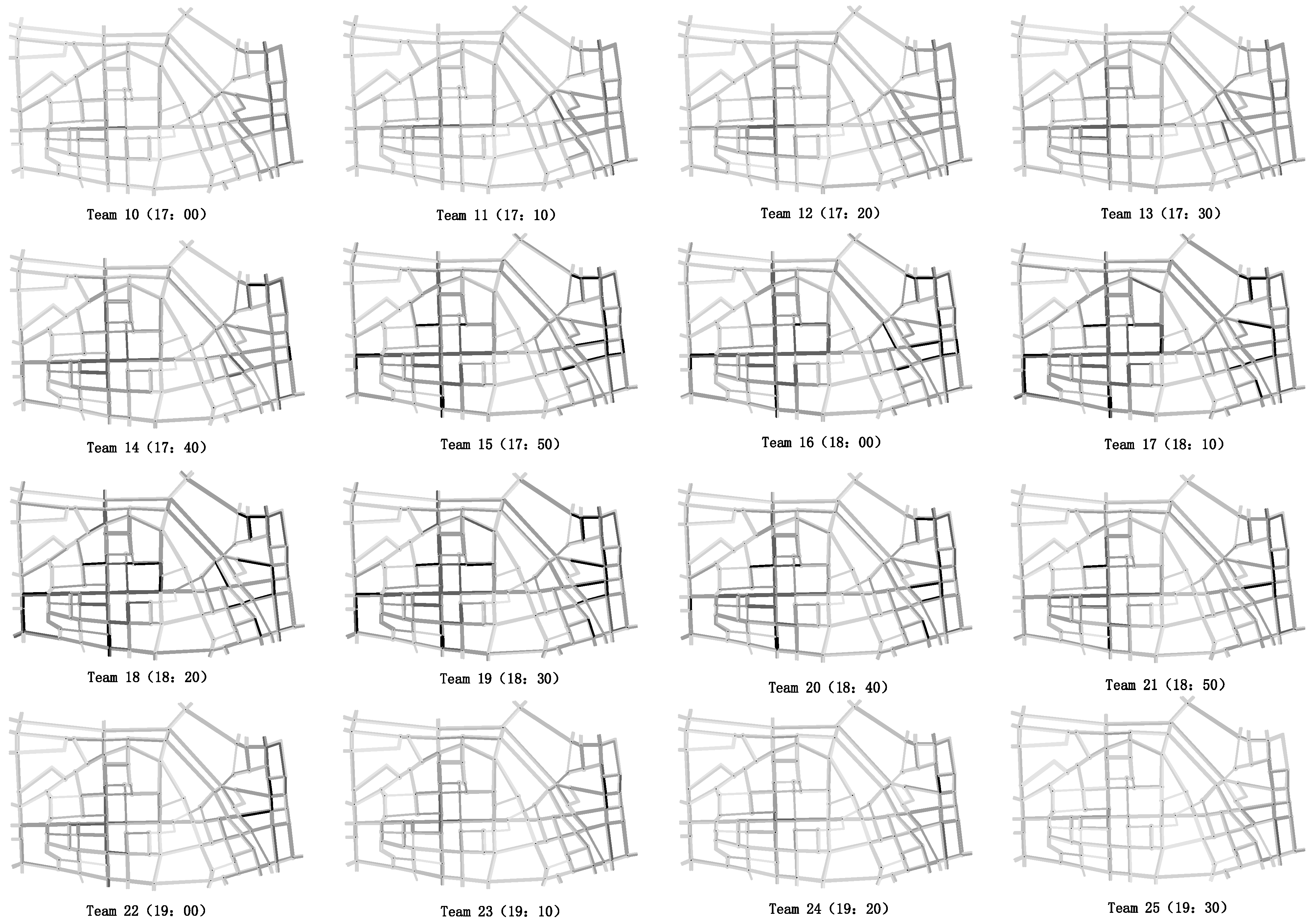
4.1. Network and Data Description

The test area is located in the city center of Xuzhou, within 4.5 square kilometers of the Second Ring Road. There are about 110 intersections and 400 sections within this area, ranging in length from 150 to 800 m. The number of lanes varies from two to four. Most traffic signals are fixed phase timing control. The calculation time of the zone partition method is in 2 s, which can be used in real-time zone partition.

Traffic density data of road sections were obtained from the calculation of GPS floating vehicle data in Xuzhou. The research team received the data of the GPS floating car in Xuzhou city on one day, which included the location coordinates, direction, speed, and other information. Through the road segment matching algorithm, traffic flow, and traffic flow velocity estimation algorithm, the traffic density parameters are obtained.

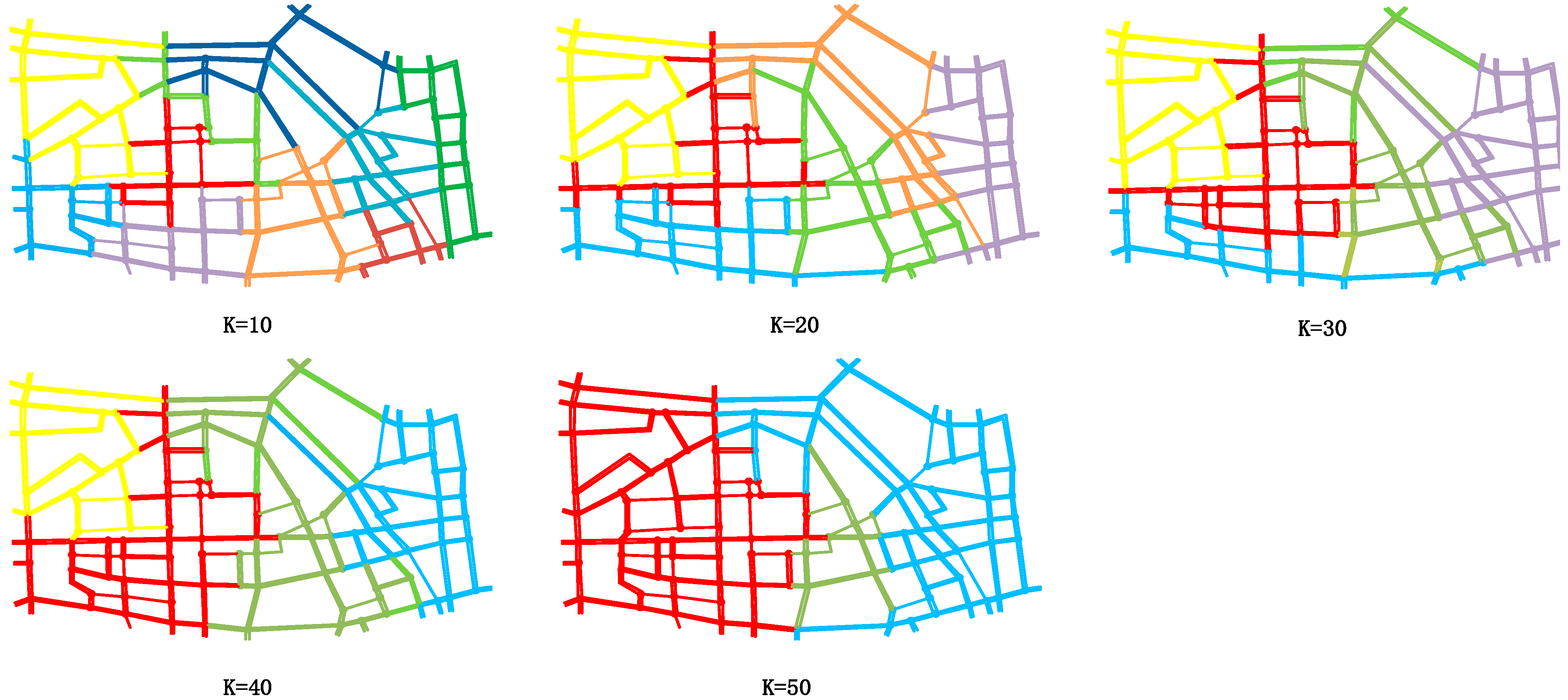
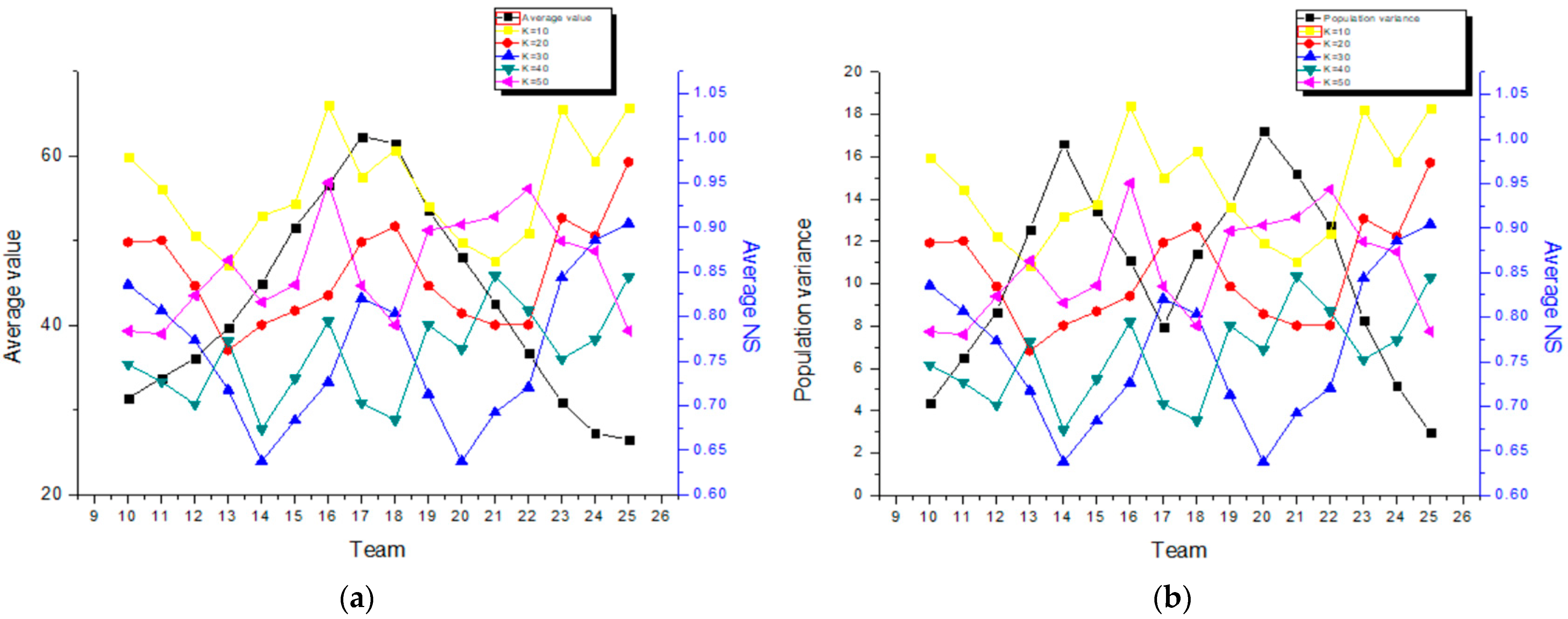
4.2. Result Analysis

To verify the reliability of the method, the traffic density changes of the road section were extracted in this area from 3:30 to 8:20 PM (evening peak-time) every 10 min, and a total of 30 sets of data were collected. From the perspective of the change of the overall network density distribution, the network traffic density starts to increase gradually from the 10th group (17:00) and presents the traffic peak at the 17th group (18:10); then, the network traffic density starts to decrease, and the traffic is stable after the 25th group (19:20). The data of 16 groups of data during the period from 17:00 to 19:20 were visualized, and a schematic diagram of the road network traffic status was drawn. The thickness of the road segment in Figure 3 represents the traffic density of the road segment. The change in road network traffic density in this period is shown in Figure 3.

It is seen from the data of the above 16 groups that the traffic network is relatively busy at the beginning and end of the evening peak, and the traffic density is not high in most sections. Similarly, at the busiest time, areas of the entire network show a higher density. The traffic density in these moments is concentrated, which is not conducive to test the reliability of this method. In the process of evening peak formation and dissipation, group 14 (17:40) is a semi-congestion network, in which the traffic density varies greatly. Therefore, this set of data is selected for research firstly.

In the above partition method, there is a parameter k about the region control, and different k values influence the partition results. Firstly, different k values are set to study the relationship between them and the partition results, which are shown in Figure 4.

Table 1. Comparison of MFD partition results in group 14 (17:40) with different k values.

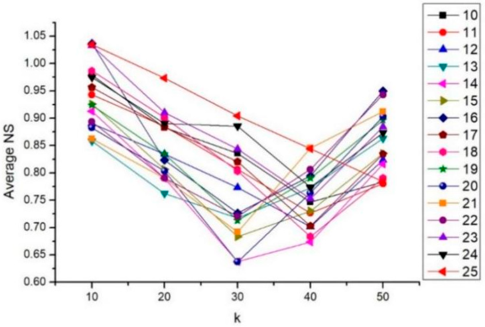
k	10	20	30	40	50
Number of clusters	10	6	5	4	3
Average NS	0.9128	0.7904	0.6375	0.6734	0.8161

shows the partition of the entire region when different k values are set. With the increase of k value, the number of molecular areas decreases gradually, and the average NS value decreases first and then, there is addition with the increase in k value. The minimum was reached at k = 30. This is because when the k value is small, there are too many sub-regions, and the difference between sub-regions is insignificant, so the average NS value is high. When the k value is immense, the region partition is too rough, and the region that should be partitioned is not partitioned, so the average NS value is also high.

It is seen that in the partition of group 14, when k = 30, the optimal partition result is obtained, and the density of road sections in the road network varies greatly. However, the density of traffic is changing throughout the road network. Along with the periodic increase and decrease in traffic flow, the density equilibrium degree of road sections in the road network varies continuously. So, under different road network states, the value of k in road network partition also varies. To further study the relationship between the value of k and NS, different amounts of k are adopted to conduct the division of traffic data during a full evening peak data. The mean value and population variance of section density in the road network at each moment were calculated, respectively, and k values of 10, 20, 30, 40, and 50 were the average NS values of the entire road network, as shown in

Table 2. Comparison of MFD partition results at night peak with different k values.

Group Number	Average Value	Population Variance	Average NS
			10	20	30	40	50
10	31.4	4.37	0.9788	0.8832	0.8357	0.7464	0.7836
11	33.8	6.48	0.9430	0.8853	0.8065	0.7266	0.78043
12	36.1	8.66	0.8902	0.8343	0.7732	0.7016	0.8235
13	39.7	12.57	0.8580	0.7621	0.7174	0.7724	0.8631
14	44.9	16.61	0.9128	0.7904	0.6375	0.6734	0.8161
15	51.6	13.43	0.9261	0.8065	0.6835	0.7302	0.8356
16	56.5	11.11	1.0367	0.8234	0.7265	0.7944	0.9501
17	62.3	7.95	0.9563	0.8834	0.8205	0.7028	0.8346
18	61.5	11.44	0.9867	0.9011	0.8034	0.6836	0.7903
19	53.6	13.63	0.9237	0.8345	0.7129	0.7904	0.8966
20	48.1	17.20	0.8827	0.8033	0.6374	0.7634	0.9032
21	42.6	15.18	0.8623	0.7904	0.6921	0.8455	0.9120
22	36.7	12.72	0.8936	0.7907	0.7204	0.8065	0.9431
23	30.9	8.28	1.0329	0.9106	0.8437	0.7523	0.8845
24	27.3	5.18	0.9744	0.8903	0.8854	0.7739	0.8732
25	26.5	2.97	1.0346	0.9734	0.9045	0.8439	0.7839

. Figure 5a shows the change of average NS value in 16 groups of data with different k values during peak hours. It is seen from Figure 5a that the average NS value has a low cost in k = 30 and k = 40, indicating that these two values may obtain better partition results. To further explore the importance of k, the changes in density mean and population variance of 16 groups of data sections during peak hours were statistically analyzed, as shown in Figure 5b. It can be seen from Figure 6 that the traffic density of evening rush hour first increases and then decreases, while the population variance value of traffic density of road sections in the road network changes in a hump shape. When the average value of NS is the lowest, the cost of k has no relation with the growth of the average vehicle density of the road section, but when the average cost of NS is the lowest, the cost of k has a significant relation with the population variance of vehicle density of the road section in the road network. Figure 6 shows that when the NS average value is the lowest, the cost of k shows a specific aggregation according to the population variance change. When the conflict is 50–150, it is easy to obtain the optimal result when k is 40, and when the population variance is more significant than 150, it is easy to obtain the optimal output when k = 3.

4.3. Method Comparison

In the introduction, two main methods of road network partition—clustering and segmentation—are mentioned. K-means in the clustering method and multiple dichotomies in the segmentation method are selected, respectively, to compare with the method proposed in this study. It is also compared with an MFD partition method based on contradiction, which consists of segmentation, merging, and boundary adjustment. We select the 14th group of data for method comparison.

In the K-means algorithm, K samples are selected randomly as the initial center in the model, and each sample is allocated to the nearest center successively, after which the clustering center is updated until the value is unchanged. In the partition of the road network, the distance between sections and the vehicle density of areas should be considered. Therefore, the vector composed of the location coordinate (x, y) at the center point of the road section and the vehicle density d of the road section is the section attribute vector (x, y, d). O_s is the coordinate weight. O_d is the density weight. In our way, 14 groups of data are finally partitioned into five clusters, so K = 5, and the initial centers are randomly set to conduct a road network partition.

Table 3. Comparison of partition results of different Os/Od ratios under the K-means method.

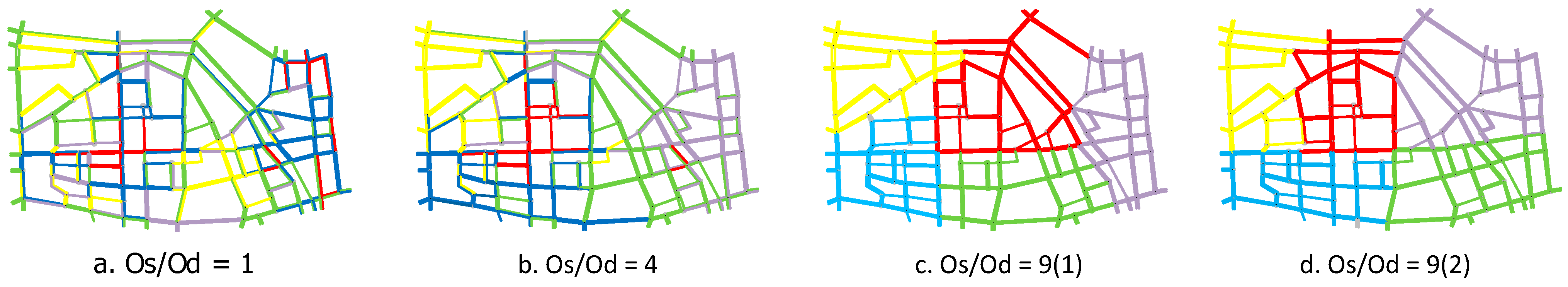
K-Means	Figure 7a	Figure 7b	Figure 7c	Figure 7d	Our Method
	Os/Od = 1	Os/Od = 4	Os/Od = 9 (1)	Os/Od = 9 (2)
Average NS	0.1046	0.6439	0.9324	1.0471	0.6375

shows the measurements. Figure 7a shows the division at Os/Od = 1. Although the average NS value is low, the division of the road network is chaotic, and an area is division into many parts, which does not help the subsequent control. Figure 7b shows the division at Os/Od = 4. It is seen that the division of the road network has become less chaotic, and some areas are still undergoing division. Figure 7c,d are two kinds of partitions in the case of Os/Od = 9. At this time, the partition area is relatively complete, but the result changes much, and the division is unstable.

Moreover, the average NS value is high, and the partition result is unsatisfactory. This situation is because K-means is not suitable for the partition of the urban traffic network, and the partitioning results of this method have a great relationship with the selection of the initial center. The connectivity of the road network was not considered in the calculation process of this method, which led to regional dispersion when the coordinate value was low. A high coordinate weight could improve the connectivity of the road network, but the average NS of the road network was high, and the partition result was unsatisfactory.

The multiple dichotomy method first divides the road network into two parts and then divides each piece separately. In the process of partition, the average NS value is taken as the measurement indicator. If the average NS after a specific sub-area is divided is higher than before, then it is considered that the sub-region has been optimally divided. Figure 8 shows the whole partition process. Figure 8a–d divide the entire road network into five groups, and the average NS value of the road network decreases gradually. Figure 8(e1–e5) show the partition result of each group after dividing into five parts.

Table 4. Results of the fifth partition.

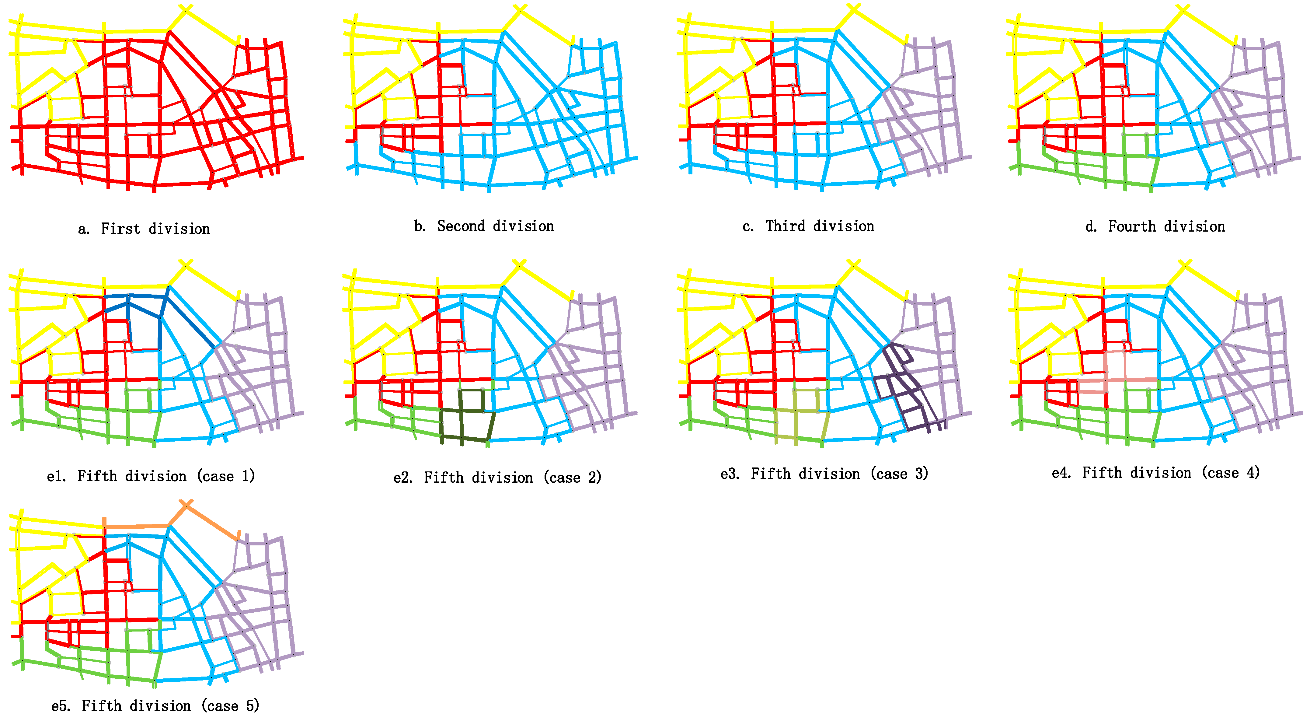
Fifth Partition	5-1	5-2	5-3	5-4	5-5
Average NS	0.7476	0.7205	0.8024	0.7706	0.7359

indicates that the NS value of any cluster will not decrease no matter which group is further partitioned, so Figure 8d shows the optimal partition result. According to

Table 5. Partition process and result comparison of numerous dichotomies.

Number of Partition	1	2	3	4	Our Method
Average NS	0.9753	0.8945	0.8105	0.7024	0.6375

, in the partition process, the NS value of the multiple dichotomy method is still more significant than the partition result of the method proposed in this study, so the road network partition method proposed in this study is better than the multiple dichotomy method. In Figure 8, the optimal partition results still show that some sections of roads in two different directions are separated, which is not conducive to further traffic control.

With the increase in the number of segmentations, the sub-regions segmented by multiple dichotomies show an exponential rise. In the segmentation results, there are a large number of sections of the same road in other directions divided into different regions at the edge of the segmentation region. Based on multiple dichotomies, Jin and Geroliminis developed a combined algorithm consisting of three computational steps: partition, merge, and boundary adjustment. In this method, the regional network is divided into several sub-regions according to the section density. After that, the adjacent regions with high similarity were merged, and the result was determined according to NS value. Finally, the boundary of the merged subregion is adjusted to optimize the shape of the region. After nine times of segmentation, we form five areas, which finally change the boundary. The critical link in the process of this method is shown in Figure 9. As can be seen from

Table 6. Comparison of combination division process and results.

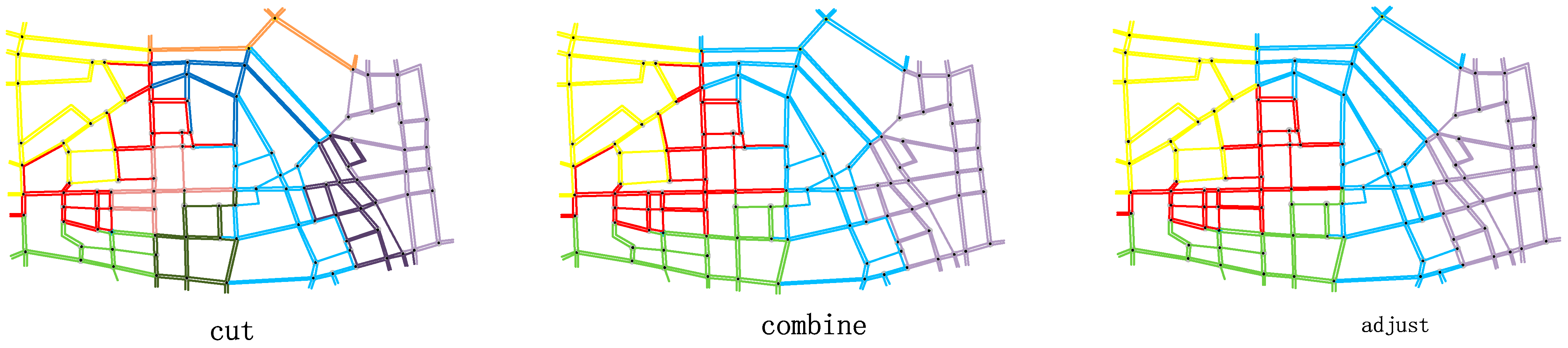
Process	Partition	Merge	Adjustment	Our Method
Average NS	0.9753	0.6724	0.7407	0.6375

, in the whole process, the number of sub-regions after segmentation is the same as in our proposed method. Comparing the NS values of the improved dichotomy and the proposed method, the average NS value of the improved dichotomy method is the lowest, but it is greater than the method we proposed. In addition, after boundary adjustment, the average NS value has risen again. Here are mainly the following factors: on the one hand, this method based on multiple dichotomy separated some areas of density concentration during the dichotomy process; on the other hand, this method separates some road sections with different driving directions during the division process, and it finally corrects them in the boundary adjustment.

5. Conclusions and Future Development

5.1. Conclusions

The proposal of MFD provides strong support for the macro-level management of urban traffic, and the application of MFD in urban traffic management requires the partition of MFD regions. This study designed an MFD partition method of urban road traffic network based on graph theory, which was different from the existing partition method aiming at road sections. The graph theory method was used to transform the road network into multiple networks connected by the vertices of the intersection and its corresponding areas, and then, the vertex network was partitioned into several parts by the minimum spanning tree method. Finally, the attribution of the boundary section was adjusted to obtain the final partition result. The relationship between the value of the regional control parameter k and the final product was explored through multiple sets of data, and the experience of selecting a particular value of k was obtained. Compared with the classical two-class partition method and a combinatorial partition method based on segmentation, the results showed that this method can obtain not only better partition results but also obtain a complete partition area, which was more conducive to signal control.

The K-means algorithm does not consider the connectivity of the road network. Multiple dichotomies and improved multiple dichotomy may separate homogeneous regions in the dichotomy process. At the same time, this type of method does not consider different driving directions on the same road and requires subsequent adjustments. The method based on graph theory overcomes the problem that different driving directions of the same road section are separated by taking the intersection as the division object. At the same time, the improved minimum spanning tree method is used to overcome the problem of homogeneous regions being separated. The experimental results further prove that the division result of our proposed method is better than existing methods.

5.2. Future Development

In this study, we only took data at an interval of 10 min according to the real-time traffic status of the road network to conduct the classification of MFD. However, in real urban traffic control, traffic control acts on the traffic flow with delay, so the regional control strategy should be maintained for at least 20 to 30 min, and further research on the zoning trigger mechanism is needed. In practical application, the traffic density data of the overall road network are in great demand, and the traffic density of each section of the road network at the same time is required. Current traffic density sources mainly include GPS floating car data and fixed traffic detection equipment [35,36]; however, due to the coverage rate and the location of the various types of testing equipment, the detection results have a more significant impact. The research on the MFD partition method, which can obtain similar partition results under limited traffic information of a road network, has excellent significance for practical application.

Moreover, the purpose of the MFD partition is to develop more effective traffic control strategies, while traffic strategies at the macro level are closely related to traffic area partition. Existing studies have found that traffic control strategies based on MFD are formulated according to the traffic status of the MFD region. Areas with heavy traffic should try to balance the distribution of traffic and control the inflow of vehicles, while areas with small traffic flow should give priority to traffic efficiency. The purpose of signal control based on MFD is to keep the traffic density in the MFD area at a specific value and maintain its shape. Then, if the MFD is partitioned by a single influencing factor of vehicle density, the congestion area will be marked out. At this time, MFD is in the hysteresis area and difficult to recover. Therefore, in the classification of MFD, whether to only consider the traffic density or to add road network, traffic flow, and other factors needs further research.

References

- Munoz, J.C.; Daganzo, C.F. Structure of the transition zone behind freeway queues. Transp. Sci. 2003, 37, 312–329. [Google Scholar] [CrossRef][Green Version]
- Daganzo, C.F. Urban gridlock: Macroscopic modeling and mitigation approaches. Transp. Res. B-Methodol. 2007, 41, 49–62. [Google Scholar] [CrossRef]
- Geroliminis, N.; Daganzo, C.F. Existence of urban-scale macroscopic fundamental diagrams: Some experimental findings. Transp. Res. B-Methodol. 2008, 42, 759–770. [Google Scholar] [CrossRef]
- Geroliminis, N.; Daganzo, C.F. Macroscopic modeling of traffic in cities. In Proceedings of the Transportation Research Board Meeting, Washington, DC, USA, 21–25 January 2007. [Google Scholar]
- Gayah, V.V.; Daganzo, C.F. Clockwise hysteresis loops in the Macroscopic Fundamental Diagram: An effect of network instability. Transp. Res. B-Methodol. 2011, 45, 643–655. [Google Scholar] [CrossRef]
- Geroliminis, N.; Boyaci, B. The effect of variability of urban systems characteristics in the network capacity. Transp. Res. B-Methodol. 2012, 46, 1607–1623. [Google Scholar] [CrossRef]
- Gan, W.J.; Gayah, V.V. A kinematic wave approach to traffic statics and dynamics in a double-ring network. Transp. Res. B-Methodol. 2013, 57, 114–131. [Google Scholar] [CrossRef]
- Buisson, C.; Ladier, C. Exploring the Impact of Homogeneity of Traffic Measurements on the Existence of Macroscopic Fundamental Diagrams. Transp. Res. Rec. 2009, 2124, 127–136. [Google Scholar] [CrossRef]
- Daganzo, C.F.; Gayah, V.V.; Gonzales, E.J. Macroscopic relations of urban traffic variables: Bifurcations, multivaluedness and instability. Transp. Res. Part B Methodol. 2011, 45, 278–288. [Google Scholar] [CrossRef]
- Tsubota, T.; Bhaskar, A.; Chung, E. Macroscopic Fundamental Diagram for Brisbane, Australia Empirical Findings on Network Partitioning and Incident Detection. Transp. Res. Rec. 2014, 2421, 12–21. [Google Scholar] [CrossRef]
- Hoai-Nam, N.; Fishbain, B.; Bitar, E.; Mahalel, D.; Gutman, P. Dynamic Model for estimating the Macroscopic Fundamental Diagram. PapersOnLine 2016, 49, 297–302. [Google Scholar] [CrossRef]
- Batista, S.F.A.; Seppecher, M.; Leclercq, L. Identification and characterizing of the prevailing paths on a urban network for MFD-based applications. Transp. Res. Part C Emerg. Technol. 2021, 127, 102953. [Google Scholar] [CrossRef]
- Gao, X.S.; Gayah, V.V. An analytical framework to model uncertainty in urban network dynamics using Macroscopic Fundamental Diagrams. Transp. Res. B-Methodol. 2018, 117, 660–675. [Google Scholar] [CrossRef]
- Shim, J.; Yeo, J.; Lee, S.; Hamdar, S.H.; Jang, K. Empirical evaluation of influential factors on bifurcation in macroscopic fundamental diagrams. Transport. Res. C-Emerg. 2019, 102, 509–520. [Google Scholar] [CrossRef]
- Yang, X.Z.; Guo, Y. Exploring the Relationship between Heterogeneity of Vehicle Distribution and the Macroscopic Fundamental Diagram under Segment Disruption Conditions. Procedia Comput. Sci. 2017, 109, 600–607. [Google Scholar]
- Wahaballa, A.M.; Hemdan, S.; Kurauchi, F. Relationship Between Macroscopic Fundamental Diagram Hysteresis and Network-Wide Traffic Conditions. Transp. Res. Procedia 2018, 34, 235–242. [Google Scholar] [CrossRef]
- Tak, S.K.; Yeo, H. Investigating Transfer Flow between Urban Networks Based on a Macroscopic Fundamental Diagram. Transp. Res. Rec. 2018, 2672, 75–85. [Google Scholar] [CrossRef]
- Jain, A.K. Data clustering: 50 years beyond K-means. Pattern Recogn. Lett. 2010, 31, 651–666. [Google Scholar] [CrossRef]
- Li, Y.; Zhu, L.; Sun, J.; Tian, Y. Generating a Spatiotemporal Dynamic Map for Traffic Analysis Using Macroscopic Fundamental Diagram. J. Adv. Transport. 2019, 2019, 9540386. [Google Scholar] [CrossRef]
- Saeedmanesh, M.; Geroliminis, N. Dynamic clustering and propagation of congestion in heterogeneously congested urban traffic networks. Transp. Res. Part B Methodol. 2017, 105, 193–211. [Google Scholar] [CrossRef]
- Saedi, R.; Saeedmanesh, M.; Zockaie, A.; Saberi, M.; Geroliminis, N.; Mahmassani, H.S. Estimating network travel time reliability with network partitioning. Transp. Res. Part C Emerg. Technol. 2020, 112, 46–61. [Google Scholar] [CrossRef]
- Lin, X. A Road Network Traffic State Identification Method Based on Macroscopic Fundamental Diagram and Spectral Clustering and Support Vector Machine. Math. Probl. Eng. 2019, 2019, 6571237. [Google Scholar] [CrossRef]
- Lentzakis, A.F.; Su, R.; Wen, C. Time-dependent partitioning of urban traffic network into homogeneous regions. In Proceedings of the International Conference on Control Automation Robotics & Vision, Singapore, 10–12 December 2014. [Google Scholar]
- Mori, G. Guiding Model Search Using Segmentation; IEEE: Piscataway, NJ, USA, 2005; pp. 1417–1423. [Google Scholar]
- Haddad, J.; Geroliminis, N. On the stability of traffic perimeter control in two-region urban cities. Transp. Res. B-Methodol. 2012, 46, 1159–1176. [Google Scholar] [CrossRef]
- Laval, J.A.; Castrillon, F. Stochastic approximations for the macroscopic fundamental diagram of urban networks. Transp. Res. B-Methodol. 2015, 81, 904–916. [Google Scholar] [CrossRef]
- Geroliminis, N.; Sun, J. Properties of a well-defined macroscopic fundamental diagram for urban traffic. Transp. Res. B-Methodol. 2011, 45, 605–617. [Google Scholar] [CrossRef]
- Geroliminis, N.; Haddad, J.; Ramezani, M. Optimal Perimeter Control for Two Urban Regions With Macroscopic Fundamental Diagrams: A Model Predictive Approach. IEEE Trans. Intell. Transp. Syst. 2013, 14, 348–359. [Google Scholar] [CrossRef]
- Aboudolas, K.; Geroliminis, N. Perimeter and boundary flow control in multi-reservoir heterogeneous networks. Transp. Res. B-Meth. 2013, 55, 265–281. [Google Scholar] [CrossRef]
- Li, D.; Liu, Z.; Lang, W.; Zhang, C.; Zhu, M.; He, Z. Consensus-Based Approach for Perimeter Control of Urban Road Traffic Networks. ACSR-Adv. Comput. Sci. Res. 2016, 52, 200–208. [Google Scholar]
- Felzenszwalb, P.F.; Huttenlocher, D.P. Efficient Graph-Based Image Segmentation. Int. J. Comput. Vis. 2004, 59, 167–181. [Google Scholar] [CrossRef]
- Van de Sande, K.E.; Uijlings, J.R.; Gevers, T.; Smeulders, A.W. Segmentation as selective search for object recognition. In Proceedings of the IEEE International Conference on Computer Vision, Barcelona, Spain, 6–13 November 2011. [Google Scholar]
- Boykov, Y.Y.; Jolly, M.P. Interactive graph cuts for optimal boundary & region segmentation of objects in N-D images. In Proceedings of the Eighth IEEE International Conference on Compoter Vision, Vancouver, BC, Canada, 7–14 July 2001; Volume I, pp. 105–112. [Google Scholar]
- Zeng, J.W.; Qian, Y.S.; Yin, F.; Zhu, L.P. A multi-value cellular automata model for multi-lane traffic flow under lagrange coordinate. Comput. Math. Organ. Theory 2021, 28, 178–192. [Google Scholar] [CrossRef]
- Knoop, S.L.L.; Keyvan-Ekbatani, M. Using Taxi GPS Data for Macroscopic Traffic Monitoring in Large Scale Urban Networks: Calibration and MFD Derivation. Transp. Res. Procedia 2018, 34, 243–250. [Google Scholar]
- Ambuehl, L.; Loder, A.; Zheng, N.; Axhausen, K.W.; Menendez, M. Approximative Network Partitioning for MFDs from Stationary Sensor Data. Transp. Res. Rec. 2019, 2673, 94–103. [Google Scholar] [CrossRef]