A Car-Following Model Based on Trajectory Data for Connected and Automated Vehicles to Predict Trajectory of Human-Driven Vehicles

Abstract

Connected and Automated Vehicles (CAV) have been rapidly developed, which, inevitably, renders that human-driven and autonomous vehicles share the road. Thus, trajectory prediction is an important research topic, which helps each CAV to efficiently follow a Human-Driven Vehicle (HV). In a wider scope, trajectory prediction, also, helps to improve the throughput of traffic flow and enhance its stability. To realize the trajectory prediction of Connected and Automated Vehicles to Human-Driven Vehicles, a car-following model, which is based on trajectory data, was established. Adding deep neural networks and an Attention mechanism, this paper established a data-driven car-following model, based on CNN-BiLSTM-Attention for CAV, to predict trajectory, by referring to the modeling idea of the traditional car-following model. The trajectory data in the next-generation-simulation (NGSIM) datasets that match the car-following characteristics were selected. In addition, noise-reduction pre-processing of the trajectory data was performed, to make it match the actual car-following situation. Experiments, for selecting the optimal structure of the model and the method of trajectory prediction, were carried out. The data-driven car-following models, such as LSTM, GRU, and CNN-BiLSTM, were selected for comparative analysis of trajectory prediction. The results show that the CNN-BiLSTM-Attention model has the smallest MAE and MSE as well as the largest R². The CNN-BiLSTM-Attention model has the highest accuracy in vehicle-trajectory prediction. The model can, effectively, realize vehicle-trajectory prediction and provide a theoretical basis for vehicle-trajectory-based velocity guidance of Human-Driven Vehicles. In the future, the model can, also, provide the theoretical basis for Connected and Automated Vehicles, to make car-following decisions in mixed traffic flow.

1. Introduction

As urbanization continues to accelerate, traffic volume is increasing, so traffic congestion and other traffic phenomena are becoming more and more significant. The car-following model is an important topic in the field of traffic flow. Studying the car-following behavior of vehicles can help to understand the operating characteristics of traffic flow and, thus, solve traffic problems, such as congestion. Over the past few decades, researchers have established several car-following models, to describe the car-following behavior of vehicles. Car-following models can be divided into two categories: mathematical car-following models and data-driven car-following models. Mathematical car-following models are models that use kinematics knowledge to construct, with a clear physical meaning. These models can, mathematically, describe car-following behavior in the context of varying traffic conditions, such as the Pipes car-following model (Pipes, 1953) [1], General Motors (GM) car-following model (Gazis et al., 1959; Gazis et al., 1961) [2,3], Helly car-following model (Helly, 1959) [4], Newell car-following model (Newell, 1961) [5], Full Velocity Difference (FVD) car-following model (Jiang et al., 2001) [6], Intelligent Driver Model (IDM) car-following model (Helbing et al., 2001) [7], Gipps car-following model (Gipps, 1981) [8], and Molecular Dynamics car-following model (Qu et al., 2017; Li et al., 2018) [9,10].

With the continuous development of intelligence, data-driven car-following models have gradually emerged. These models are based on trajectory data, to complete the modeling. The models can fully explore the connection between the data, so the models can accurately predict the car-following behavior of the vehicles.

Connected and Automated Vehicles (CAV) have been rapidly developed, which, inevitably, renders that human-driven and autonomous vehicles share the road. Due to the difference between the car-following characteristics of CAV and Human-Driven Vehicles (HV), the car-following behavior of mixed traffic flow is somewhat different from that of purely human-driven traffic flow. CAV can obtain operational information on HV through onboard sensors, roadside sensors, and communication devices. They can make car-following decisions, by predicting the trajectories of other HV. Accurate and quick trajectory prediction can help to reduce traffic accidents, improve the throughput of traffic flow, and enhance its stability and safety. The car-following models can be applied to trajectory prediction. Although the mathematical car-following models are widely applied and are interpretable, they cannot be useful in the long term. In addition, it is difficult to obtain the exact operation of surrounding vehicles, so the mathematical car-following models are less effective in real traffic flow. To accurately obtain the actual operation of the surrounding vehicles and improve the prediction accuracy in the actual traffic flow, the numbers of data-driven car-following models have, gradually, been applied. Deep learning is considered as a nonlinear-function approximator, for mapping nonlinear functions, which is superior in terms of prediction effectiveness and performance. A variety of neural networks, such as the convolutional neural network (CNN), recurrent neural network (RNN), and long short-term memory (LSTM) network, have been applied to natural-language processing, image recognition, and time-series analysis. CAV can use the learning capability of deep neural networks to learn the driving skills of HV, based on historical trajectory data [11].

The rest of the paper is organized as follows: Section 2 reviews the studies about data-driven car-following models and prediction of trajectory. The preprocessing of trajectory data of vehicles is presented in Section 3. Section 4 presents the design idea and theoretical basis for establishing the sequential model. In Section 5, experiments are conducted to set the parameters of the model and to select the optimal model’s structure and method of predicting trajectory. Section 6 presents the results of the model for predicting trajectory as well as the comparison with other data-driven car-following models, and the experimental results of experiments are analyzed and discussed. Section 7 gives the conclusion.

2. Literature Review

Kehtarnavaz et al., (1998) used a Back Propagation (BP) neural network to establish a car-following model [12]. Jia et al., (2001) established a model based on BP-neural-network theory, to simulate car-following behavior [13]. Wei and Liu (2013) established a car-following model based on the theory of support-vector regression, and the error-evaluation index showed that the model has high evaluation accuracy [14]. Zhou et al., (2017) proposed the RNN-based car-following model [15]. Since the input variables consider the time-series data, the model can obtain the driver’s reaction time and has a better prediction ability. The model can better reproduce the traffic oscillation and distinguish the driver’s characteristics. Wang et al., (2018) applied the GRU neural-network structure to model the car-following behavior [16]. Huang et al., (2018) proposed a car-following model, based on an LSTM neural network [17]. The simulation results showed that the LSTM-NN model could better capture asymmetric driving behavior. Sun and Guo (2020) established a car-following model, based on an LSTM neural network [18]. The car-following model was trained with actual vehicle-trajectory data. The results showed that the LSTM-based car-following model is stable, and it can dissipate a disturbance in traffic flow. In addition, the model has good anti-interference ability and predictive effect. Fei et al., (2020) constructed a car-following model, based on the GRU network, and conducted simulation experiments to verify the validity of the model [19]. It was confirmed that the model has high robustness and improved simulation accuracy, compared with the traditional models.

In terms of the prediction of trajectory, Lu (2017) proposed a data-driven car-following model, considering driving-behavior constraints, which can be used for traffic simulation, to realize trajectory prediction [20]. Zhou et al., (2017) proposed an RNN-based car-following model, which has a good ability to reproduce traffic oscillation [15]. The method of trajectory prediction was selected through experiments. Huang et al., (2018) designed a single-lane driving-simulation experiment. The first vehicle drove with the observed data, and the subsequent car-following vehicles all drove with the established LSTM-NN car-following model. The simulation results showed that the model can realize trajectory prediction [17]. Deo et al., (2018) applied an LSTM neural network, to achieve trajectory prediction of the vehicle on the highway [21]. Altche et al., (2017) used an LSTM neural network for highway-trajectory prediction and applied the trajectory data in the NGSIM dataset for validation [22]. Zhang et al., (2019) established a two-channel fusion model, based on CNN- and LSTM-neural-network structure, which can extract data features and realize prediction [23]. Kim et al., (2017) proposed a method to predict the position of vehicles, based on a deep dynamic neural network, which is an LSTM. The inputs of the LSTM neural network were the coordinates and velocities of the surrounding vehicles [24]. Xie et al. [25,26,27] proposed an improved constrained sparse auto-encoder and correlation-analysis method, for diagnosing intermittent fault problems, while instrument fault problems are solved effectively with the advantages provided by deep learning. Based on recurrent neural networks and convolutional neural networks, Wang et al., (2021) proposed a fusion neural-network architecture, called F-Net, for vehicle trajectory prediction on the highway and urban scenarios in autonomous-driving applications [28]. Rossi et al. (2021) compared deep-learning models, based on LSTM and Generative Adversarial Network (GAN) architectures; in particular, the GAN-3 model can be used to generate multiple predictions in multimodal scenarios [29].

From previous studies, data-driven car-following models could effectively predict the driver’s car-following behavior and the trajectory of the vehicle. Most of the previous studies use a single moving model to realize the prediction of car-following behavior and trajectory, which lacks timeliness and accuracy. Based on the results of previous studies, we can obtain that CNN can extract the features of input data. BiLSTM is capable of processing long time-series data, selectively acquiring and forgetting the historical information, which is consistent with the human-driving process, in which drivers make decisions based on different short-term memories. BiLSTM can fully extract data features in both positive and negative directions. An Attention mechanism means that the human brain responds to specific information processing, by focusing its attention on key areas to obtain important information. The Attention mechanism can enhance the importance of important parts of the input features. Therefore, this paper constructed a car-following model that combines CNN, LSTM, and the Attention mechanism, for CAV to predict the trajectory of surrounding HV. The CNN-BiLSTM-Attention model combines the characteristics of CNN, LSTM, and the Attention mechanism, which can effectively extract the input data features and strengthen the focus on important features. The model can overcome the shortcomings of the single-moving model, such as insufficient timeliness and accuracy.

In this paper, we screen the trajectory data in the NGSIM dataset that match the car-following characteristics and pre-process the screened trajectory data, by moving the smoothing method with noise reduction. Adding a deep-learning network and the Attention mechanism, we establish a data-driven car-following model based on CNN-BiLSTM-Attention, for CAV to predict trajectory, by referring to the modeling idea of the traditional car-following model. We select the optimal network structure of the model and the trajectory-prediction method through experiments. We compare the performance of CNN-BiLSTM-Attention with other data-driven car-following models, such as LSTM, gated recurrent unit (GRU), and CNN-BiLSTM, in terms of trajectory prediction.

3. Data Processing

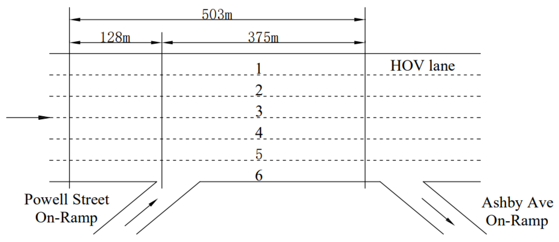
To realize the trajectory prediction of CAV to HV, a large amount of HV trajectory data is necessary for training the model. This paper uses the vehicle-trajectory data collected from the eastbound direction of the California I-80 highway, in the NGSIM (Next Generation Simulation) project, as the dataset. The data were acquired by seven cameras erected on a high-rise building, adjacent to the I-80 highway, at a frame rate of 10 frames per second. The section of I-80 used for data collection is 503 m long, with six lanes. Lane 1 is a highoccupancy vehicle lane (HOV), and lane 6 is an on-ramp. The specific situation of the I-80 road section is shown in Figure 1.

This paper studies the car-following behavior and microscopic characteristics of vehicles. In order to obtain enough trajectory data of traffic oscillation, the trajectory data of the collection period, from 05:00 p.m. to 05:15 p.m., are selected. The condition of the road is congestion during this period, which can fully reflect the traffic-flow condition of acceleration change. This dataset has 1836 vehicles, with 1,549,918 trajectory records, and the temporal interval of the data is 0.1 s. To obtain sufficient trajectory data, in line with the car-following characteristics of the vehicle, to complete the training and calibration of the car-following model, the above-mentioned dataset needs to be screened. The principles are as follows:

(1)

To avoid the differences in car-following characteristics caused by different vehicles, screen vehicles with class 2, and eliminate class 1 and class 3 vehicles, which represent motorcycles and large vehicles, respectively;

(2)

To ensure consistent driving behaviors, eliminate vehicles in lane 1 and lane 6, to ensure consistent driving behaviors;

(3)

Eliminate vehicles with no vehicles in front and rear;

(4)

To avoid the impact of lane-changing, screen vehicles that have not changed lanes;

(5)

Eliminate trajectory data with headway less than 5 m and more than 60 m, which can be considered as car-following behavior that has been released;

(6)

Screen the trajectory data with a car-following time longer than 60 s, to ensure the complete car-following process and sufficient trajectory data.

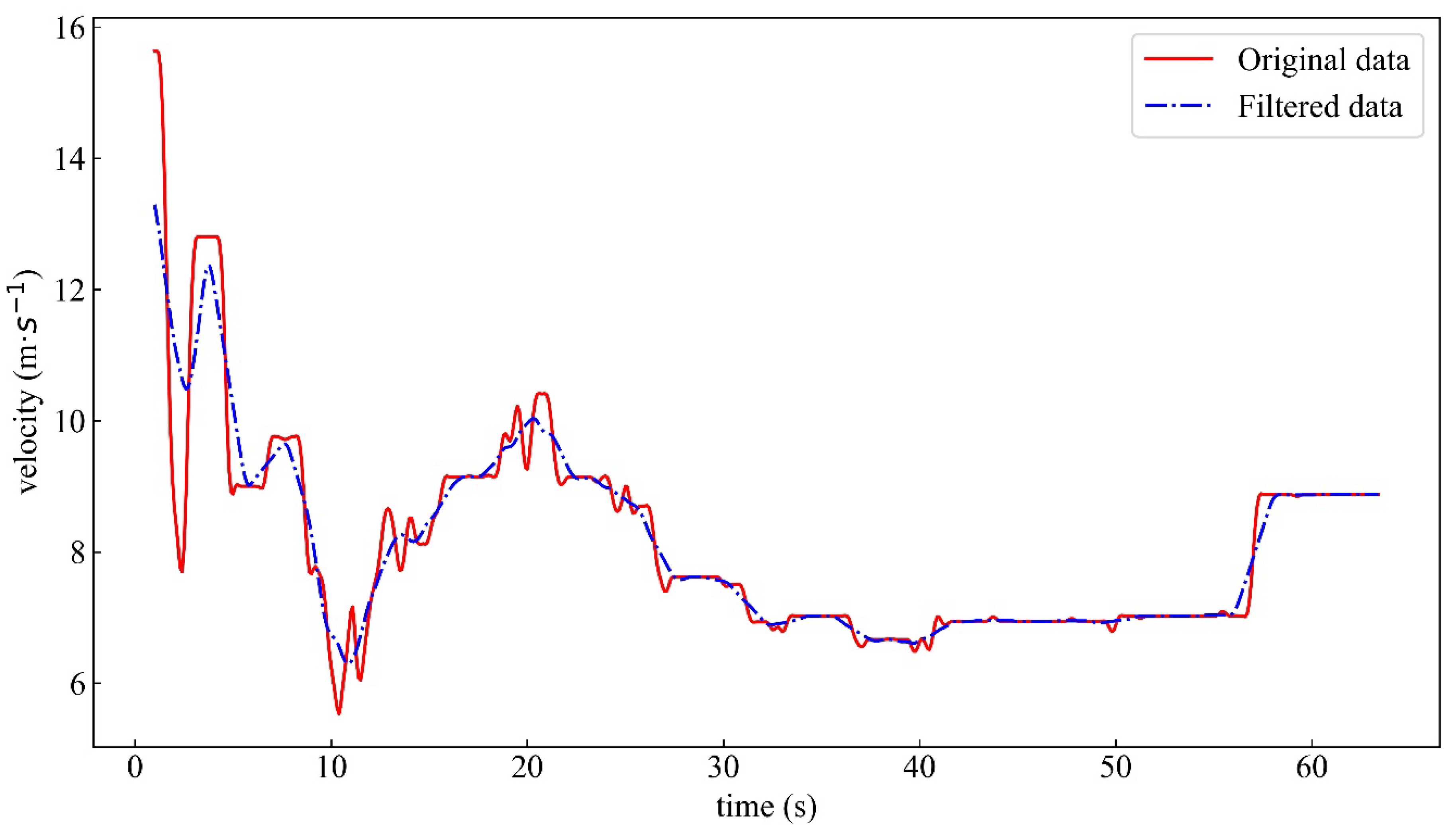
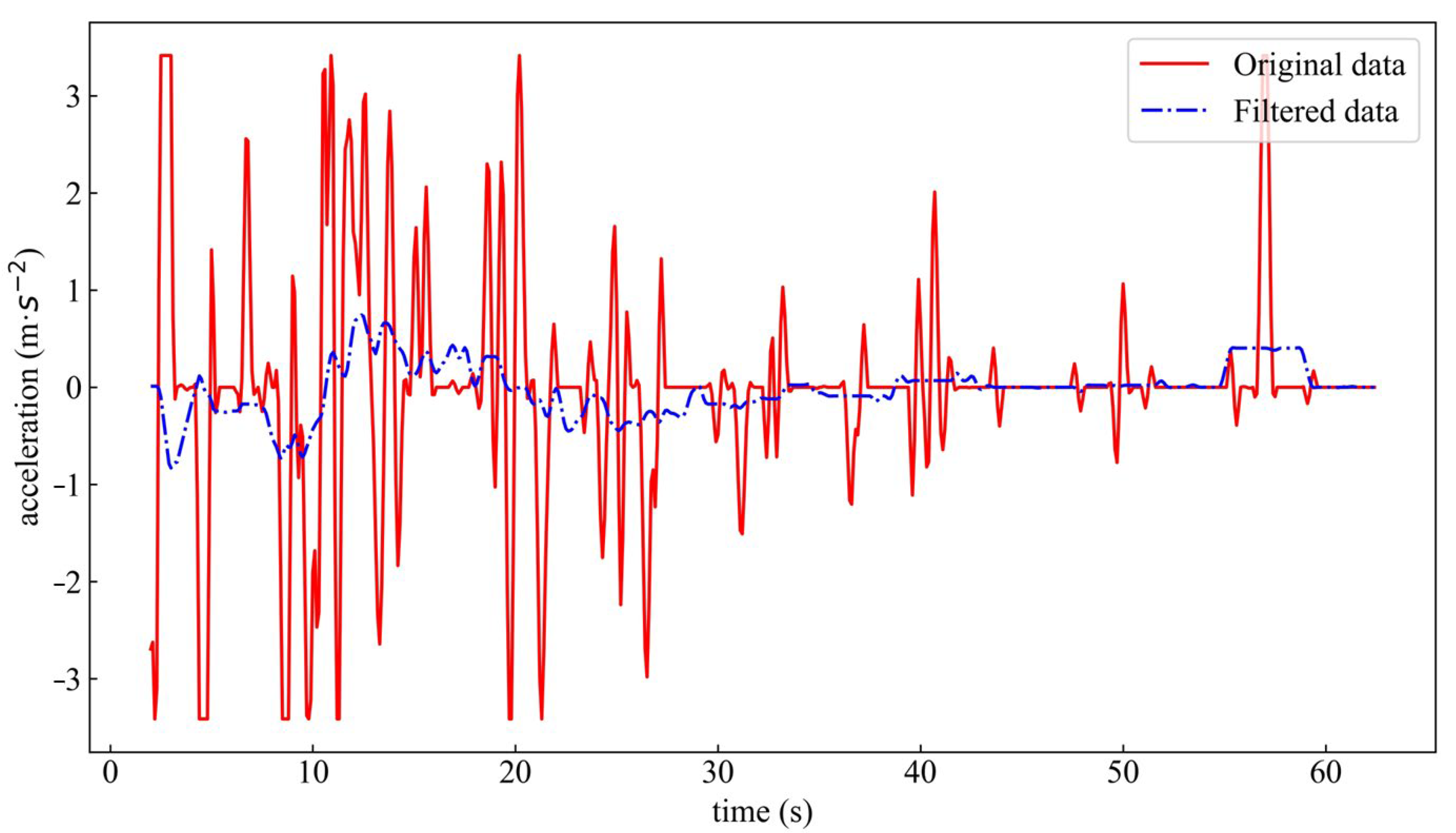
The dataset is obtained by extracting video images through computer recognition technology. There are many measurement errors and abnormal values, such as the velocity distribution, which change frequently and tend to be a specific value. The velocity changes are not smooth. Vehicles frequently accelerate and decelerate, with the maximum acceleration in the data within two adjacent seconds (Punzo et al., 2011; Montanino and Punzo, 2013) [30,31]. It cannot conform to the actual driving behavior and cannot meet the demand of vehicle-micro-behavior characteristics research, so data noise reduction is required. The data noise reduction is completed by the moving average (Thiemann et al., 2008) [32]. Taking the vehicle with VehicleID 295, as an example, the noise-reduction results of velocity and acceleration are shown in Figure 2 and Figure 3.

A total of 266,778 pieces of data are obtained, after screening and noise reduction. In addition, 80% of the data are used for model training. The remaining 20% are used for model verification.

The pre-processed data are normalized, to map the original data to between (0–1), to eliminate the influence of dimensions. The formula is as shown in Equation (1).

$$x^{\ast }=\frac{x-x_{\min }}{x_{\max }-x_{\min }}$$

(1)

where x_max denotes the maximum value in the original data, x_min denotes the minimum value in the original data.

4. Trajectory-Prediction Model

In previous studies, trajectory prediction can be realized by establishing deep-learning networks. Through deep learning, we can acquire nonlinear functions that approximate the real data. Deep-learning theory has made great progress in the field of artificial intelligence. In this section, we combine neural networks, such as CNN, BiLSTM, and the Attention mechanism, to establish the CNN-BiLSTM-Attention model that can be applied to Connected and Automated Vehicles. The applied theories include the CNN model, the BiLSTM neural network, and the Attention mechanism.

4.1. CNN Model

CNN is an NN structure, proposed by Lecun and Bottou [33]. The CNN model is used in related fields, such as image recognition, speech recognition, and traffic-flow prediction [34,35]. The CNN model is composed of an input layer, an output layer, and several hidden layers. The cores of the hidden layer are a convolutional layer and a pooling layer, which can extract data features and reduce the amount of data, thereby increasing the training velocity. Take the third-order convolution kernel as an example: the operation of the convolutional layer is shown in Figure 4, and the formula is as shown in Equation (2).

$$c_{ij}={\omega }_{11}{x}_{ij}+{\omega }_{12}{x}_{i\left(j+1\right)}+\cdots {\omega }_{33}{x}_{\left(i+2\right)\left(j+2\right)}$$

(2)

where c_ij denotes convolution result, ω denotes value of convolution kernel, and x denotes input data.

The pooling layer performs feature selection to reduce the amount of data, to obtain strong features and improve the resistance of the network to interference. The equation of the pooling layer is as shown in Equation (3).

$$z_i=pool\left(j_i\right)$$

(3)

where z_i denotes output of pooling layer, j_i denotes input of pooling layer, and pool denotes pooling operation.

The CNN model can realize features extraction of input data and deeply mine the internal connection of input features, so we chose the CNN model for modeling.

4.2. BiLSTM Neural Network

LSTM was introduced in 1997, by Hochreiter and Schmidhuber [36]. The LSTM neural network, with the forgetting gate, can obtain historical information. When the historical information is out of date, the memory module can be reset and gradually removed. It is very consistent with the process of human driving. The driver can make decisions, based on different short-term historical information.

The LSTM model is composed of an input layer, a hidden layer, and an output layer. The hidden layer is mainly used for feature learning of input data. The memory module is the main unit. The LSTM unit contains a forgetting gate f_t, an input gate i_t, and an output gate o_t. The forgetting gate controls the information forgotten by the cell state c_t−1 at time t − 1. The input gate controls the information, by inputting x_t into cell state c_t at time t. The output gate controls the information about the cell state c_t entering the hidden state h_t at time t. The structure of the LSTM unit is shown in Figure 5.

$$f_t=\sigma \left(W_{if}{x}_t+b_{if}+W_{hf}{h}_{t-1}+b_{hf}\right)$$

(4)

$$i_t=\sigma \left(W_{ii}{x}_t+b_{ii}+W_{hi}{h}_{t-1}+b_{hi}\right)$$

(5)

$$o_t=\sigma \left(W_{io}{x}_t+b_{io}+W_{ho}{h}_{t-1}+b_{ho}\right)$$

(6)

$${\tilde{c}}_t=\tanh \left(W_{ic}{x}_t+b_{ic}+W_{hc}{h}_{t-1}+b_{hc}\right)$$

(7)

$$c_t=f_t\times c_{\mathrm{t}-1}+i_t\times {\tilde{c}}_t$$

(8)

$$h_t=o_t\times \tanh \left(c_t\right)$$

(9)

σ denotes siomoid activation function, as shown in Equation (10):

$$\sigma =\frac{1}{1+e^{-x}}$$

(10)

tanh denotes activation function, as shown in Equation (11):

$$\tanh \left(x\right)=\frac{e^x-e^{-x}}{e^x+e^{-x}}$$

(11)

where W denotes weight matrix, b denotes bias.

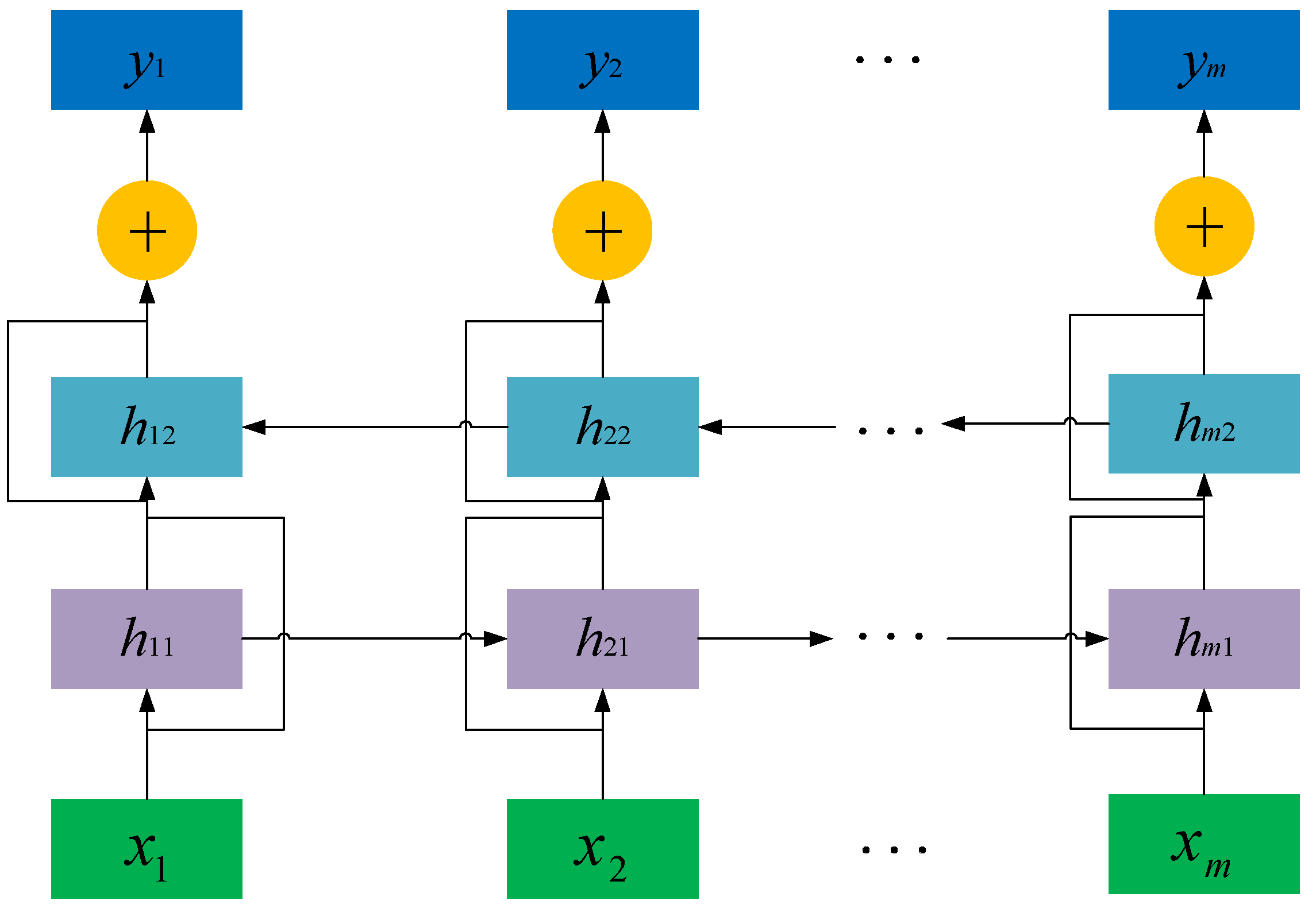
LSTM can only obtain the historical information coming from the forward transmission, which leads to a lag in the prediction process. BiLSTM consists of two LSTM neural network units in opposite directions, which can, simultaneously, consider the information of data in both forward and backward directions as well as predict data in both directions. Two independent hidden layers can process the data in both directions, separately. The output is determined by the output in both directions, thereby reducing the prediction error, so the BiLSTM neural network is selected for modeling. The structure of BiLSTM is shown in Figure 6.

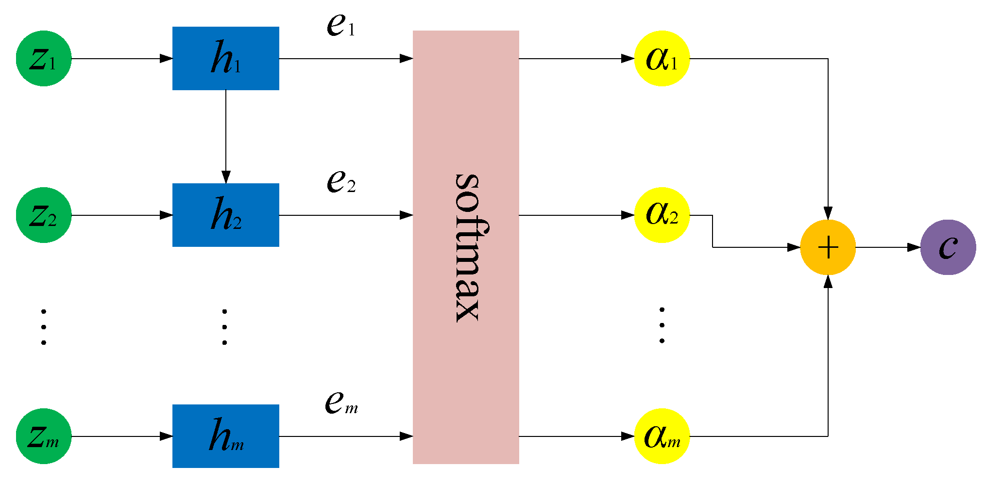
4.3. Attention Mechanism

The Attention mechanism refers to the fact that the human brain processes specific information, by focusing its attention on key regions, to obtain important information. (Cui et al., 2020) [37]. The attention mechanism assigns weight to the input features, thus focusing on the important parts of the input features. The structure is shown in Figure 7.

$$e_t=v\tanh \left(W{h}_t+b\right)$$

(12)

$${\alpha }_t=\frac{\exp e_t}{{\displaystyle \sum _{j=1}^n{e}_j}}$$

(13)

$$c_t={{\displaystyle \sum _{j=1}^n{\alpha }_j{h}_j}}_{ }$$

(14)

where e_t denotes the weight corresponding to the feature at time t, α_t denotes the attention weight corresponding to feature at time t, v and W denote the shared weight, b denotes bias, and c_t denotes the output at time t.

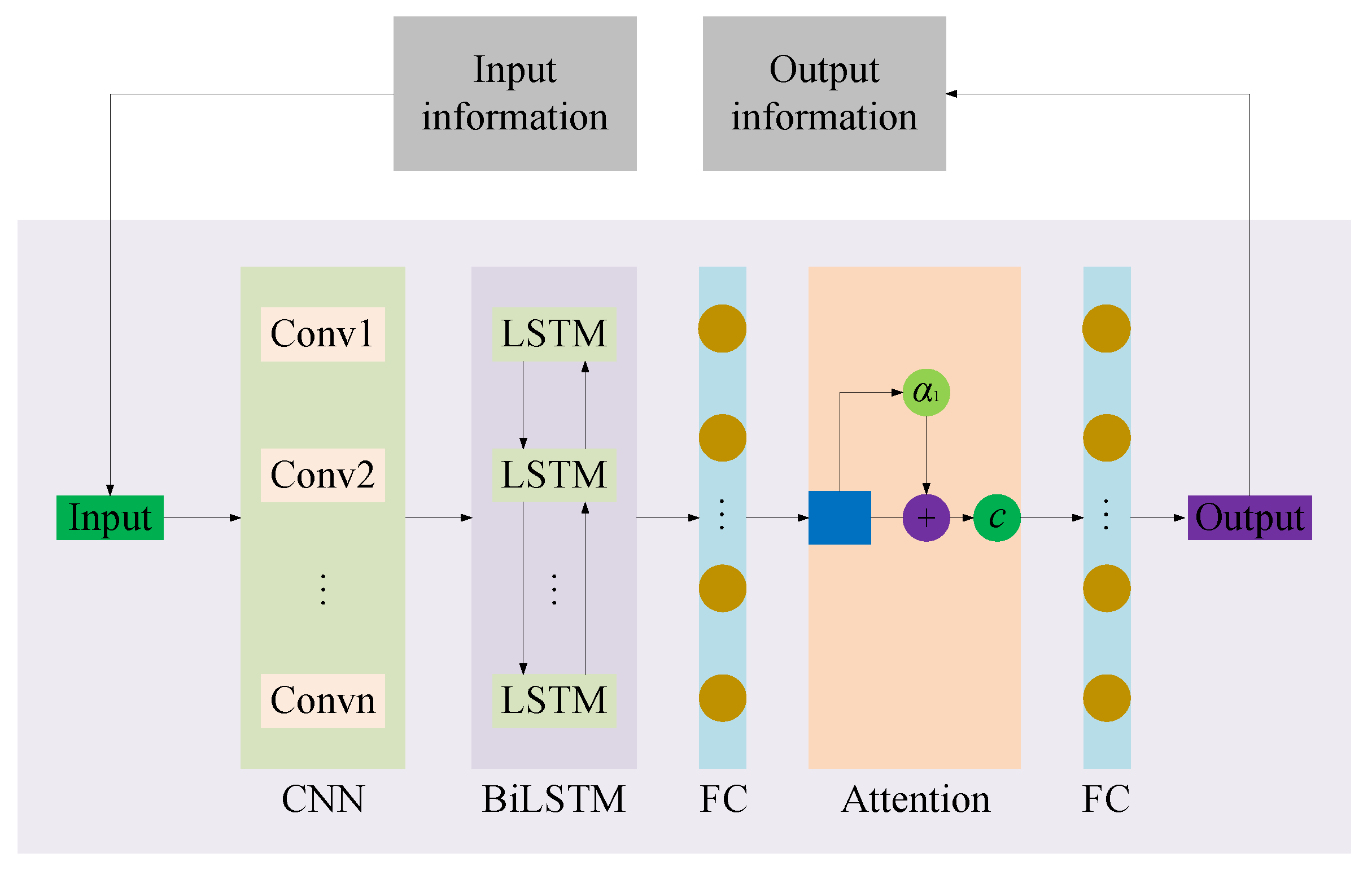
4.4. CNN-BiLSTM-Attention Car-Following Model

Keras is used to construct and train the CNN-BiLSTM-Attention-based car-following model. TensorFlow is used for the backend.

The structure of the CNN-BiLSTM-Attention car-following model is shown in Figure 8.

The CNN-BiLSTM-Attention model is composed of a CNN layer, a BiLSTM layer, an Attention layer, and two fully connected layers. The CNN layer can extract input data features of trajectory data and, then, is connected to the BiLSTM network, which can fully extract forward and reverse features as well as obtain the short-term temporal feature of trajectory data. Then, a fullyconnected layer (FC) is followed, which is the regression layer, to perform forecasting. In addition, the Attention layer is connected to the fullyconnected layer (FC), which can automatically explore different levels, of the importance of flow sequences at different times, and strengthen the model’s attention to important features. Finally, the other fullyconnected layer (FC) is followed.

5. Settings of Model

5.1. Indicators of Evaluation

Select mean absolute error (MAE), coefficient of determination (R²), and mean square error (MSE) as evaluation indicators, as shown in Equations (15)–(17).

$$\mathrm{MAE}=\frac{1}{n}{\displaystyle \sum _{i=1}^n\left|\left(y_{\mathrm{i}}-{\tilde{y}}_i\right)\right|}$$

(15)

$${\mathrm{R}}^2=1-\frac{{\displaystyle \sum _{i=1}^n{\left({\tilde{y}}_i-y_i\right)}^2}}{{\displaystyle \sum _{i=1}^n{\left({\overline{y}}_i-y_i\right)}^2}}$$

(16)

$$\mathrm{MSE}=\frac{1}{n}{{\displaystyle \sum _{i=1}^n\left(y_i-{\tilde{y}}_i\right)}}^2$$

(17)

where n denotes total number of evaluation data samples, y_i denotes true value of evaluation data, ${\overline{y}}_i$ denotes the mean value of the true value of evaluation data, and ${\tilde{y}}_i$ denotes predicted value.

5.2. Parameter Settings

The model’s parameters determine the prediction accuracy. To improve the model’s accuracy of prediction, the CNN layer’s convolutional kernel size is set to 1 × 1, the convolutional step size is set to 1, the activation function is set to ReLU, the optimizer is selected to Adam, the loss function is set to MSE, and the batch size is selected to 64, through experimental verification. Settings of the hyperparameters are shown in

Table 1. Hyperparameters settings.

Parameter	Setting	Parameter	Setting
Kernel size	1 × 1	Optimizer	Adam
Convolution step	1	Loss function	MSE
Activation function	ReLU	Batch size	64

.

Choosing the appropriate input and output can improve the accuracy of the model. Referring to the modeling idea of the GM (Gazis et al.,1961) model, we chose v_n+1(t), Δv(t), and Δx(t) as input as well as a_n+1(t + Δt) as output. The objective function is as shown in Equation (18).

$$a_{n+1}\left(t+\Delta t\right)=f\left(v_{n+1}\left(t\right),\Delta v\left(t\right),\Delta x\left(t\right)\right)$$

(18)

where $f(·)$ denotes the function of mapping relationship between input and output variables, v_n+1(t) denotes the velocity of the following vehicle at time t, Δv(t) denotes the relative velocity of two vehicles at time t; Δx(t) denotes the gap of two vehicles at time t, and a_n+1(t + Δt) denotes the acceleration of the following vehicle at time t + Δt.

The decision in car-following is closely dependent on historical driving behavior. The historical time step is the length of time of the entered historical data. The historical time step affects the prediction accuracy of the model. The optimal historical time step and the optimal model structure are determined experimentally.

Firstly, the model structure is fixed. To save training time, both CNN and BiLSTM choose a simple structure, with a single hidden layer with 64 neurons. In addition, the historical time steps of 1 s, 3 s, 5 s, 7 s, and 10 s are experimented with, to determine the optimal time steps, based on MSE. The temporal interval of the data is 0.1 s, which means a time step is 0.1 s. The results are shown in Figure 9. The optimal time step is 5 s, which is 50 time steps.

The models with different structures are designed for experiments, and the model with the highest prediction accuracy is selected, based on the indicators of the evaluation. The number of convolution kernels is 64 for 1-layer CNN 64 and 64 for 2-layer CNN, and 64, 64, and 128 for 3-layer CNN. The number of units in each layer of BiLSTM is 64. The specific settings are shown in

Table 2. Depth and width settings of CNN model and BiLSTM model.

Number of CNN Layers	Number of Convolution Kernels			Number of BiLSTM Units
1			64	64
2		64	64	64
3	128	64	64	64

.

Experiments are conducted for models with different structures, and the comparison results are shown in

Table 3. Structure of model.

Number of CNN Layers	Number of BiLSTM Layers	MAE	R2	MSE
1	1	0.0412	0.9269	0.0123
	2	0.0635	0.9158	0.0142
	3	0.0410	0.9243	0.0127
2	1	0.0428	0.9271	0.0123
	2	0.0474	0.9272	0.0123
	3	0.0409	0.9259	0.0125
3	1	0.0444	0.9231	0.0130
	2	0.0373	0.9290	0.0120
	3	0.0432	0.9263	0.0124

.

According to Table 3, the model has the smallest MAE and MSE as well as the largest R², when the number of CNN layers is 3 and the number of BiLSTM layers is 2, which is determined as the best structure of the model.

5.3. Selection of Prediction Methods

There are the following methods for vehicle-trajectory prediction. Trajectory prediction, which is achieved by predicting acceleration and velocity, as well as displacement that can be obtained from acceleration, such as Zhou et al. (2017) [15]. Vehicle-trajectory prediction, which is achieved by predicting vehicle displacement, such as Zhang et al. (2019) [38] and Guo et al. (2020) [39]. In this paper, the above two trajectory-prediction methods are compared and experimented with, to select the optimal trajectory-prediction method.

5.3.1. Prediction of Acceleration

According to the predicted acceleration a_n+1(t + Δt), the velocity v_n+1(t + Δt) and displacement x_n+1(t + Δt) of the rear vehicle in the next time interval can be obtained, so that the trajectory of the rear vehicle can be predicted. The objective function is as follows:

$$v_{n+1}\left(t+\Delta t\right)=v_{n+1}\left(t\right)+a_{n+1}\left(t+\Delta t\right)\Delta t$$

(19)

$$x_{n+1}\left(t+\Delta t\right)=x_{n+1}\left(t\right)+v_{n+1}\left(t\right)\Delta t+\frac{a_{n+1}\left(t+\Delta t\right)}{2}\Delta t^2$$

(20)

5.3.2. Prediction of Displacement

For the prediction of displacement, the following-vehicle velocity v_n+1(t), the velocity difference between two vehicles Δv(t), and the distance between two vehicles Δx(t) can be obtained, to ensure the same inputs and avoid the potential errors caused by different inputs. The output is the displacement of the following vehicle at the next time interval. The objective function is as follows:

$$x_{n+1}\left(t+\Delta t\right)=f\left(v_{n+1}\left(t\right),\Delta v\left(t\right),\Delta x\left(t\right)\right)$$

(21)

5.3.3. Comparative Selection

The two methods of trajectory prediction are compared, and the method with higher accuracy will be selected. To verify the accuracy of the model’s prediction for traffic oscillation, the vehicle experiencing traffic oscillation is selected for trajectory prediction. The trajectory data for VehicleID 2061 is selected. The effect of trajectory prediction, shown in Figure 10a, is the result of the prediction of acceleration, while Figure 10b is the result of the prediction of displacement.

The comparison of indicators of the evaluation is shown in

Table 4. Comparison of predicting methods.

Predicting Methods	Indicators of the Evaluation
	MAE	R2	MSE
Prediction of acceleration	0.3802	0.9907	151.5851
Prediction of displacement	2.1978	0.9894	168.8228

.

It can be seen from Figure 10 that the trajectory-curve-fitting degree of acceleration prediction is higher. It means that the accuracy of prediction is higher. It can be seen from Table 4 that the MAE and MSE of the prediction of acceleration are lower than that of the prediction of displacement, and the R² is higher than that of the prediction of displacement. The accuracy of the prediction of acceleration is higher than that of the prediction of displacement, so the prediction of acceleration is selected as the trajectory-prediction method.

6. Experimental Results and Discussion

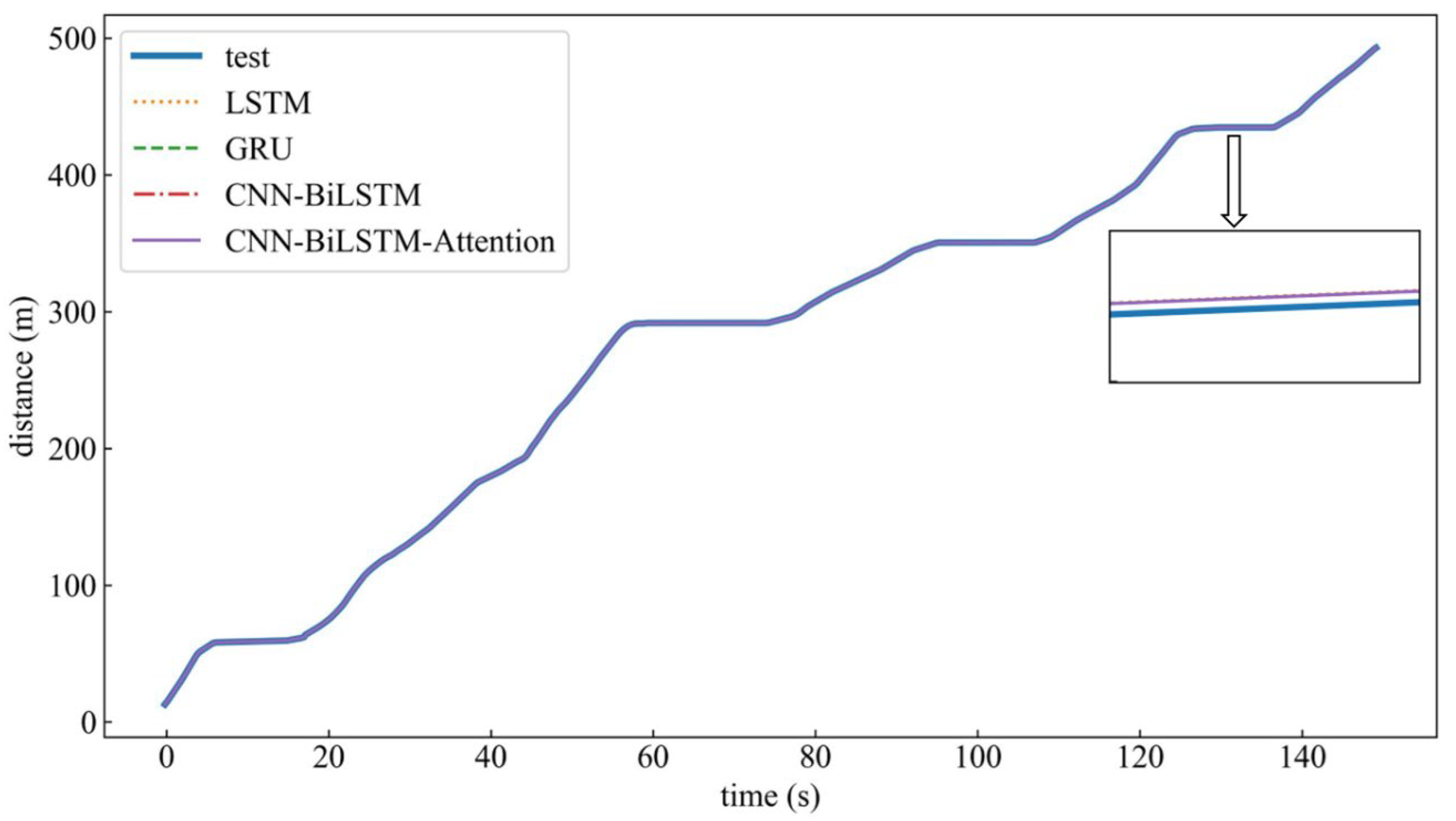
The model established in this paper belongs to data-driven car-following models. The LSTM model and GRU model have been verified to be effective and can realize trajectory prediction of vehicles. To verify the accuracy of the trajectory prediction of the car-following model, based on CNN-BiLSTM-Attention, the LSTM model and the GRU model are selected, for comparison and analysis. In order to verify the influence of the Attention mechanism on the accuracy of the prediction of trajectory, the CNN-BiLSTM model is selected, for comparison and analysis.

LSTM and GRU both set two hidden layers, with 64 neurons per layer. The rest of the parameter settings are the same as the CNN-BiLSTM-Attention model. CNN-BiLSTM has the same settings as CNN-BiLSTM-Attention, except that the Attention layer is not added. To ensure fairness, the input and output of the model are kept the same. In addition, the indicators of evaluation are MAE, R², and MSE. Select the trajectory data of the vehicle with VehicleID 2061. The effect of the comparison of each model is shown in Figure 11.

According to Figure 11, the LSTM model, GRU model, CNN-BiLSTM model, and CNN-BiLSTM-Attention model can better predict the trajectory of the vehicle. However, according to the local enlarged figure in Figure 11, the accuracy of prediction of the CNN-BiLSTM-Attention model is better than the other models.

Table 5. Evaluation of model prediction.

Model	Indicators of Evaluation
	MAE	R2	MSE
LSTM	0.3892	0.9905	151.6522
GRU	0.3892	0.9905	151.6513
CNN-BiLSTM	0.3892	0.9905	151.6512
CNN-BiLSTM-Attention	0.3802	0.9907	151.5851

shows the results of the prediction and evaluation of the total sample. According to Table 5, the CNN-BiLSTM-Attention model has the smallest MAE and MSE as well as the largest R². This model has the highest accuracy for the trajectory prediction of vehicles. The CNN-BiLSTM-Attention car-following model is better than other car-following models, in predicting the trajectories of vehicles. Compared with the LSTM model, MAE is decreased by about 2.31%, R² is increased by about 0.02%, and MSE is decreased by about 0.04%. Compared with the GRU model, MAE is decreased by about 2.31%, R² is increased by about 0.02%, and MSE is decreased by about 0.04%. Compared with the single moving models, the CNN-BiLSTM-Attention model has the characteristics of the single moving models, but the CNN-BiLSTM-Attention model can better extract features of data and process the relationships among the historical data, to capture historical information and make decisions accordingly. Compared with the CNN-BiLSTM model, MAE is decreased by about 2.31%, R² is increased by about 0.02%, and MSE is decreased by about 0.04%, indicating that the accuracy of the model’s prediction is improved, due to the Attention mechanism highlighting important features. The model proposed in the paper can compensate for the lack of timeliness and precision performance of a single moving model.

7. Conclusions

In this paper, the trajectory data of vehicles in NGSIM that meet the car-following characteristics were screened. The noise-reduction process was applied to the screened data, to obtain the dataset. The optimal structure of the model and the method of trajectory prediction were determined through experiments. Combined with the idea of the GM car-following model, the trajectory of the vehicle can be predicted, by taking the velocity of the following vehicle v_n+1(t), the velocity difference between two vehicles Δv(t), and the distance between two vehicles Δx(t) as the input, and the acceleration of the rear vehicle at the next time interval a_n+1(t + Δt) as the output, so the CNN-BiLSTM-Attention car-following model was established. The car-following model, based on CNN-BiLSTM-Attention, can be applied to the prediction of the trajectory of HV by CAV. The established car-following model was compared with the LSTM car-following model, the GRU car-following model, and the CNN-BiLSTM car-following model. The results show that the car-following model, based on CNN-BiLSTM-Attention, for Connected and Automated Vehicles, has higher accuracy of prediction. The car-following model, based on CNN-BiLSTM-Attention, for Connected and Automated Vehicles, which was established in this paper, can realize the prediction of trajectory in traffic congestion. Vehicles can be guided in velocity, based on the predicted trajectory, so the car-following model can reduce traffic congestion and improve the operational efficiency of traffic flow. In the era of continuous development of Connected and Automated Vehicles, there will be a mixed traffic flow composed of CAV and HV, for a long time in the future. The model established in this paper can provide the predicted trajectory of HV for CAV, which can help CAV to make decisions and improve the stability of traffic flow in the process of car-following.

There are some limitations in this paper. Deep-learning neural networks can extract important data features from the data and enhance the focus on important data features, to get higher prediction accuracy. However, the interpretation ability of deep-learning networks is not strong, and we cannot know which data features are important. We apply the deep-learning neural networks, to establish a car-following model to achieve trajectory prediction, according to their characteristics. The data selected in this paper are from the NGSIM dataset, and the trajectory data of the HV in NGSIM are applied to train the model. The car-following characteristics of vehicles in different regions are different. The car-following characteristics of the HV in the networked mixed traffic flow, also, differ from those of the vehicles in the purely human-driven traffic flow. The selected trajectory data cannot fully reflect the car-following characteristics of HV in mixed traffic flow and do not apply to all regions. In the future, the model can be trained with trajectory data from different regions, to verify the applicability of the model in different regions. In the future, the model can be trained with the trajectory data in the networked mixed traffic flow, to verify the accuracy of the prediction of the model for HV in the mixed traffic flow. In addition, this paper excludes the impact of lane-changing on driving behavior. In the future, the CNN-BiLSTM-Attention model can be used to predict both longitudinal and lateral driving behavior. The complex network structure not only ensures high accuracy of prediction but also increases the training time of the model. In the future, the model will be continuously improved to reduce the training time, while ensuring the accuracy of prediction. CAV can obtain the information about multiple vehicles. However, in this paper, only the information from the vehicle ahead is considered. How to achieve the prediction of trajectory for CAV to HV, by the information of multiple vehicles, is our next research topic.