Forecasting Daytime Ground-Level Ozone Concentration in Urbanized Areas of Malaysia Using Predictive Models

Abstract

Ground-level ozone (O₃) is one of the most significant forms of air pollution around the world due to its ability to cause adverse effects on human health and environment. Understanding the variation and association of O₃ level with its precursors and weather parameters is important for developing precise forecasting models that are needed for mitigation planning and early warning purposes. In this study, hourly air pollution data (O₃, CO, NO₂, PM₁₀, NmHC, SO₂) and weather parameters (relative humidity, temperature, UVB, wind speed and wind direction) covering a ten year period (2003–2012) in the selected urban areas in Malaysia were analyzed. The main aim of this research was to model O₃ level in the band of greatest solar radiation with its precursors and meteorology parameters using the proposed predictive models. Six predictive models were developed which are Multiple Linear Regression (MLR), Feed-Forward Neural Network (FFANN), Radial Basis Function (RBFANN), and the three modified models, namely Principal Component Regression (PCR), PCA-FFANN, and PCA-RBFANN. The performances of the models were evaluated using four performance measures, i.e., Mean Absolute Error (MAE), Root Mean Squared Error (RMSE), Index of Agreement (IA), and Coefficient of Determination (R²). Surface O₃ level was best described using linear regression model (MLR) with the smallest calculated error (MAE = 6.06; RMSE = 7.77) and the highest value of IA and R² (0.85 and 0.91 respectively). The non-linear models (FFANN and RBFANN) fitted the observed O₃ level well, but were slightly less accurate compared to MLR. Nonetheless, all the unmodified models (MLR, ANN, and RBF) outperformed the modified-version models (PCR, PCA-FFANN, and PCA-RBFANN). Verification of the best model (MLR) was done using air pollutant data in 2018. The MLR model fitted the dataset of 2018 very well in predicting the daily O₃ level in the specified selected areas with the range of R² values of 0.85 to 0.95. These indicate that MLR can be used as one of the reliable methods to predict daytime O₃ level in Malaysia. Thus, it can be used as a predictive tool by the authority to forecast high ozone concentration in providing early warning to the population.

1. Introduction

Ground-level ozone (O₃) is an important component of the atmosphere because it is a major oxidant and a greenhouse gas [1,2]. At ground-level, O₃ is seen in the form of a secondary atmospheric pollutant created by a number of chemical reactions that are typically linked to degradation of air quality in the air [3], which leads to adverse effects on the health of human beings, crop production, material quality, and ecosystems. High concentration of ground-level ozone can affect human health via short-term and long-term impacts. Short-term impacts include mortality and breathing morbidity and are likely to lead to eye irritation and can also influence the airway [4], while lung damage and inflammatory reactions can be caused over the long term [5].

Ground-level O₃ is one of the global air pollution problems. In Malaysia, since 1997, ground-level O₃ has been recognized as one of the significant contaminants of air due to the growing ozone precursors [6]. Rapid economic development and high emissions of pollutants in nearby urban and industrialized areas were detected as the main contributors to the increase in O₃ precursors such as NOx, VOCs, and CO. The main sources of O₃ precursors were reported to be industrial and vehicle emission [6]. Vehicle emission can lead to high emission of NO due to higher titration processes between NO and O₃. VOCs, that often found in urban and industrial areas, in the other hand, lead to the formation of peroxy radical (RO₂) that later undergoes photoreaction to produce O₃ [7].

Thus, due to its long- and short-term impacts on human health, the variation and relations of ground-level ozone and its precursors require much investigation [8]. Nowadays, the number of studies reported on O₃ concentration in Asia has increased, particularly in Malaysia. The monitoring data in several large cities demonstrated that O₃ level are increasing and are not always at acceptable concentration in accordance with the Malaysia Ambient Air Quality Standard (MAAQS). Thus, it is very important to understand the behavior of ground-level ozone in order to explain the association of O₃ level with its precursors and weather parameters [9].

Forecasting high ozone concentration events using mathematical tools is very useful in providing early warning to the population. However, the prediction of ground-level O₃ is more complicated due to its origin as a secondary pollutant if compared to modeling primary pollutants such as particulate matter (PM₁₀) [10]. Thus, statistical approaches had been widely used by the researchers to study the variation of O₃ concentration with its precursors and weather parameters. Multiple linear regression is one of the most common techniques used in the prediction of ground level O₃ level. The objective is to model a linear relationship between the explanatory (independent) and the answer (dependent) variables, thus the relationship of O₃ level and other variables (including other air pollutants, its precursors and meteorology parameters) can be observed [10]. In several studies conducted by Hassanzadeh et al. [11], Barrero et al. [12], Banja et al. [13], and Allu et al. [14], the connection between weather parameters and ozone concentration in Portugal, Spain, Albania, and India has been described respectively. Even though many studies have been carried out in the world investigating the association between the weather and the ozone concentration using MLR, in southeast Asia in particular there is still a shortage of work. While certain studies have been conducted by Azmi et al. [15] and Awang et al. [16], their study only focused on the trend or variation of ozone concentration in Klang Valley, Malaysia. However, there are a few studies on O₃ level prediction in Malaysia. Abdullah et al. [17] studied the high night-time O₃ concentrations in Kemaman, Terengganu, while Ghazali et al. [18] related the nitrogen dioxide transformation into the ozone and predict the ozone concentration using the multiple linear regression techniques.

Besides giving a simple linear relationship of ozone concentration with its precursors and weather parameters, linear regression may not provide accurate predictions in some complex situations such as non-linear data and extreme values data. Machine learning is an effective technique for understanding the inter-dependence of climatic data and air pollution since it supports exploratory analysis of data without using an empirical model [19,20]. Further, machine learning addresses the non-linearity problem, enhancing the model’s predictive performance [21,22]. Artificial neural networks (ANN), one of the most common machine learning techniques, can be a useful tool to extract information from imprecise and non-linear data such as air quality and meteorology. Currently, the applications of machine learning neural networks have become more popular for predicting ground-level O₃ concentration. A lot of researchers have effectively adopted ANN as a predictive tool to model O₃ concentration [23,24,25,26].

Modification of MLR and ANN has been conducted by many researchers to increase the accuracy of the predicted model. One of the main disturbances that will cause a reduction in the performance of the model and reduce the efficiency of the model is multicollinearity [27,28]. To deal with multidimensional issues and overcome feature redundancy, many researchers suggested various techniques for dimension reduction and feature extractions. One of the widely employed methods for these purposes is the principal component analysis (PCA) [29,30]. Basically, modification by substituting the input into principal components was accomplished. Most of the research had successfully increased the accuracy of the predictive models for particulate matter or O₃ level by modifying the input of regression models using principal components [9,31,32,33]. However, there were also some studies that reported the opposite results, where MLR predicts the air pollutant concentration better than PCR [1,34]. A modified model of ANN (using PCs as input to train and validate FFANN model) was implemented to increase the accuracy of the model. A few studies have applied the modified FFANN model with PCA and successfully increased the accuracy of the model in predicting PM₁₀ level [31,35] and ground-level O₃ concentration [25,36,37].

Recently, despite the superiority of ANN algorithm, other machine learning algorithms such support vector regression (SVR) and support vector machine (SVM) have become popular options among researchers due to their architectural simplicity and precision [38,39]. Balogun and Tella [40] applied four machine learning algorithms (Random Forest, Decision Tree Regression, Linear Regression, and Support Vector Regression) to predict O₃ level limited to the west coast region of peninsular Malaysia. Ayman et al. [41] applied six machine learning algorithms, namely Linear Regression (LR), Tree Regression (TR), Support Vector Regression (SVR), Ensemble Regression (ER), Gaussian Process Regression (GPR), and Artificial Neural Networks models (ANN) to model only an urban area in Malaysia, i.e., Lembah Kelang. They reported that the proposed models were capable of predicting the concentrations with higher accuracy level.

Despite these sophisticated methods, there is a lack of comprehensive studies on O₃ level prediction that involve most of the urban areas in Malaysia. Hence, thorough study on suitability of using established linear and non-linear model in predicting O₃ level in Malaysia is much needed to investigate the best method that can be used as a reliable predictive tool to estimate O₃ level. In this research, linear and non-linear models with their modified models were developed and evaluated using performance indicators. The best model selected from this study is ready to be used by the authorities as the predictive strategy of Malaysia and will be very helpful in understanding how these elements interact with O₃ content.

2. Materials and Methods

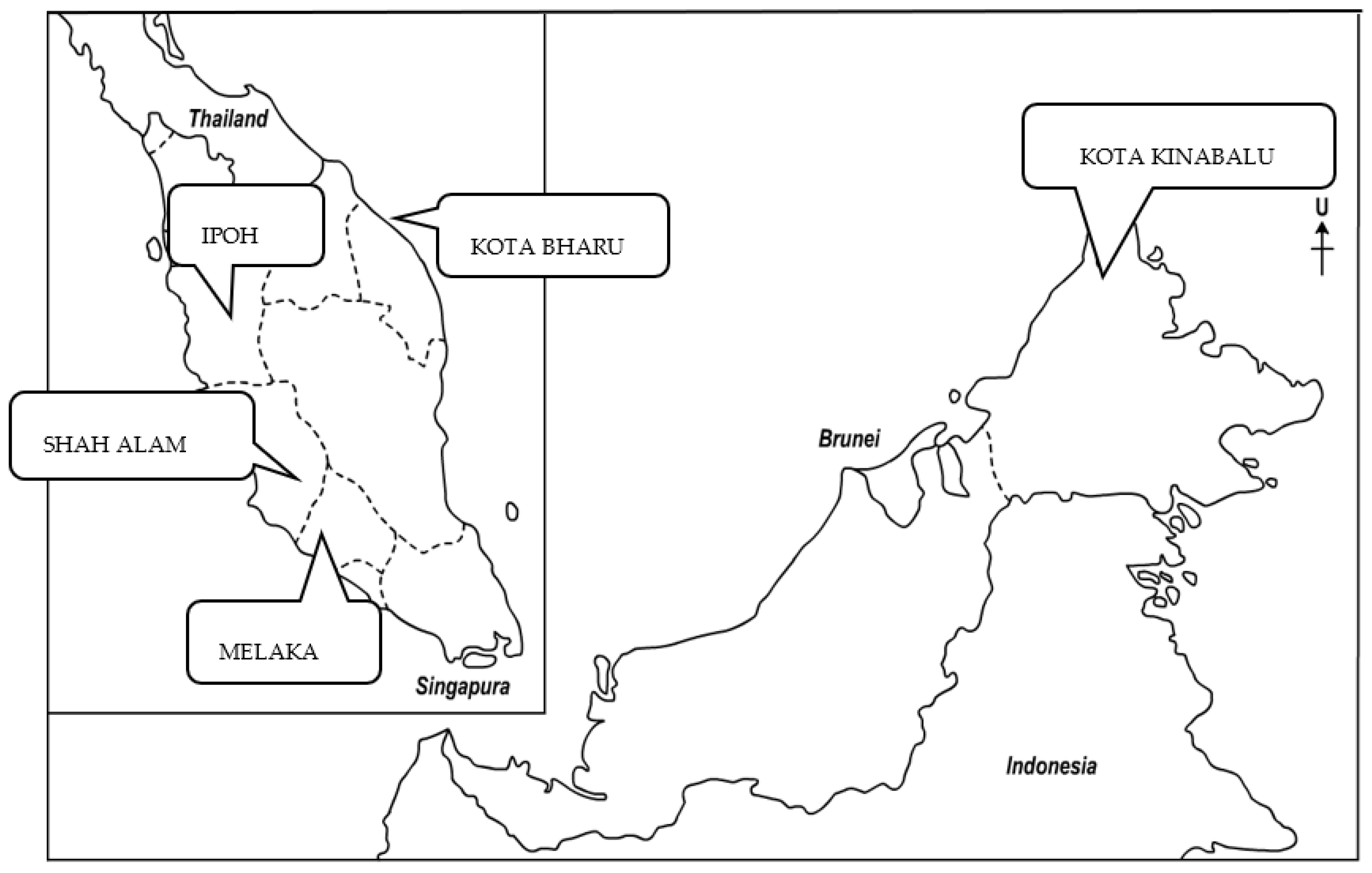
2.1. Study Area

In this study, five urban areas in Malaysia were selected. Four out of five locations are located in Malaysia’s peninsula and one station is situated in East Malaysia (Kuching). The four locations in peninsular Malaysia are distributed in the north (Perai) the center (Shah Alam), the south (Melaka), and the east (Kuala Terengganu) of peninsular Malaysia.

The selected air quality monitoring stations are displayed in Figure 1, while

Table 1. Locations and the description of monitoring stations.

Region	Monitoring Site	Latitude, Longitude	Area Description
North	Ipoh	N 4.6305, E 101.1178	Urban area Residential area
Center	Shah Alam	N 3.1066, E 101.5573	Urban area Residential area Near industrial area
South	Melaka	N 2.1919, E 102.2545	Urban area Residential area Near industrial area
East Peninsular	Kota Bharu	N 6.1464, E 102.2481	Urban area Residential area
East Malaysia	Kota Kinabalu	N 5.9532, E 116.0551	Urban area Residential area

provides a description and locations of all stations covered in this study. All the sampling sites are located in schools that are closed to residential areas. However, all of these areas are surrounded by the urban center and residential areas.

2.2. Air Pollutant Dataset

The air quality data were gathered from the Air Quality Division of the Department of Environment (DoE), Malaysia. The data were collected and monitored by Alam Sekitar Malaysia Sdn. Bhd. (ASMA), the authorized agency for DoE. The equipment used by ASMA to monitor the air quality data is from Teledyne Technologies Inc. USA (Thousand Oaks, CA, USA), and Met One Instrument Inc. USA (Grants Pass, OR, USA). Based on the Standard Operating Procedures for Continuous Air Quality Monitoring (2007), the analyzer used by ASMA to monitor PM₁₀ was a BAM-1020 Beta Attenuation Mas Monitor from Met One Instrument, Inc. USA. This instrument has a high resolution of 0.1 μg m⁻³ at a 16.7 L min⁻¹ flow rate, with lower detection limits of <4.8 μg m⁻³ and <1.0 μg m⁻³ for 1 h and 24 h, respectively. The instruments used by ASMA to monitor SO₂, CO, and O₃ were the Teledyne API Model 100A/100E, Teledyne API Model 200A/200E, Teledyne API Model 300/300E, and Teledyne API Model 400/400E, respectively, from Teledyne Technologies Inc., USA [1], while SO₂ measurement was based on the UV fluorescence method, where the lowest level of detection is at 0.4 ppb. CO was measured using the non-dispersive, infrared absorption (Beer Lambert) method with 0.5% precision and the lowest detection of 0.04 ppm. Ozone concentration was measured through the UV absorption (Beer Lambert) method with a detection limit of 0.4 ppb. The measurements of SO₂, CO, and O₃ were at a precision level of 0.5%. For NmHC, the analyzer used by ASMA measured using a Teledyne API M4020 from Teledyne Technologies Inc., USA, which is equipped with aflame-ionization detector (FID) and a measurement accuracy of 1%. These instruments were used due to well-proven accuracy, reliability, and robustness.

In this study, two sets of air pollutants data were used. The first set of data was identified based on the availability of data from 1 January 2003 to 31 December 2012. These long-term datasets were used to develop the prediction models of the daytime O₃ level. The predicted models were then validated using several performance measurements. The air pollutants (O₃, PM₁₀, NO₂, SO₂, NmHC, and CO) and weather parameters (WS, WD, H, T, and UVB) used in this research are tabulated in

Table 2. The units of air pollutants and weather parameters.

Air Pollutant/Weather Parameters	Unit
Ground-level ozone (O3)	ppb
Nitrogen dioxide (NO2)	ppm
Carbon monoxide (CO)	ppm
Sulphur dioxide (SO2)	ppm
Particulate matter (PM10)	(µg/m3)
Non-methane Hydrocarbon (NmHc)	ppm
Ambient temperature (T)	°C
Humidity (H)	%
Wind speed (WS)	km/h
Wind direction (WD)	degree (o)
Ultraviolet radiation (UVB)	W/m2

.

Table 3. Descriptive statistics (mean ± standard deviation) of air pollutants and weather parameters from 2003 to 2012. O₃: ozone; PM₁₀: particulate matter; CO: carbon monoxide; SO₂: sulphur dioxide; NO₂: nitrogen dioxide; and NmHC: non-methane hydrocarbons.

Area/Parameter	Ipoh	Shah Alam	Melaka	Kota Bharu	Kota Kinabalu
Wind Speed (km/h)	9.18 ± 2.71	8.75 ± 2.26	8.70 ± 2.77	8.47 ± 3.33	8.73 ± 2.26
Temperature (°C)	33.39 ± 2.36	32.81 ± 2.47	31.60 ± 1.74	30.78 ± 79.55	31.59 ± 2.31
Solar Radiation (W/m2)	677.27 ± 183.81	533.16 ± 191.70	Not Available	553.42 ± 215.86	668.93 ± 7.98
Humidity (%)	56.88 ± 8.66	59.37 ± 9.74	61.87 ± 8.50	63.26 ± 10.24	68.93 ± 7.98
NmHC (ppm)	0.13 ± 0.056	0.22 ± 0.12	Not Available	0.20 ± 0.11	Not Available
SO2 (ppm)	0.0018 ± 0.0012	0.0038 ± 0.0037	0.0022 ± 0.0021	0.00064 ± 0.0010	0.00055 ± 0.00070
NO2 (ppm)	0.0093 ± 0.0039	0.012 ± 0.0074	0.0043 ± 0.0021	0.0054 ± 0.0035	0.0022 ± 0.0019
CO (ppm)	0.43 ± 0.19	0.51 ± 0.34	0.32 ± 0.19	0.46 ± 0.22	0.23 ± 0.12
PM10 (µg/m3)	43.96 ± 19.17	47.23 ± 32.21	34.98 ± 21.25	35.62 ± 13.55	29.55 ± 12.56
O3 (ppb)	27 ± 6.1	31 ± 7.6	20 ± 6.5	18 ± 5.6	15 ± 3.9

shows the summary of the mean and standard deviation for hourly dataset of the air pollutants and weather parameters at the five study areas from 2003 to 2012. These long-term data were used to develop the prediction models to estimate the hourly O₃ level in the band of great solar intensity.

As for the model deployment, the prediction models (developed from previous dataset) were later deployed on the 2018 dataset.

Table 4. The mean and standard error of all the parameters at the five stations in 2018.

Area/Parameter	Ipoh	Shah Alam	Melaka	Kota Bharu	Kota Kinabalu
Wind Speed (km/h)	8.38 ± 3.19	8.14 ± 2.81	8.62 ± 2.94	7.98 ± 3.35	8.82 ± 2.37
Temperature (°C)	33.37 ± 2.62	32.81 ± 2.63	31.46 ± 1.89	30.58 ± 2.54	31.97 ± 2.38
Solar Radiation (W/m2)	742.25 ± 195.66	592.80 ± 187.38	Not Available	596.79 ± 197.86	619.79 ± 192.54
Humidity (%)	57.67 ± 8.94	59.35 ± 9.99	62.31 ± 9.10	63.87 ± 11.03	67.64 ± 7.96
NmHC (ppm)	0.13 ± 0.06	0.24 ±0.12	Not Available	0.19 ± 0.09	Not Available
SO2 (ppm)	0.0019 ± 0.0015	0.0037 ± 0.004	0.0021 ± 0.0026	0.0057 ± 0.001	0.005 ± 0.007
NO2 (ppm)	0.0094 ± 0.0051	0.012 ± 0.0089	0.0044 ± 0.0026	0.005 ± 0.0038	0.0021 ± 0.019
CO (ppm)	0.416 ± 0.202	0. 535 ± 0.348	0.328 ± 0.193	0.443 ± 0.233	0.234 ± 0.128
PM10 (µg/m3)	45.12 ± 22.66	47.34 ± 32.27	35.02 ± 22.10	36.35 ± 17.18	29.90 ± 15.37
O3 (ppb)	39 ± 16.0	52 ± 32.0	34 ± 11.0	24 ± 9.0	22 ± 6.0

shows the mean and standard deviation for hourly dataset at the five selected areas in 2018. Statistically, no significant differences were detected among the variables in 2018 when comparisons were made with the identical variables from the previously presented dataset. Verification of the best prediction model aimed to prove that the model was still reliable in predicting daytime O₃ level in different years.

In this study, the multivariate air pollutant data were treated as cross sectional data which focus on observing information of air pollutants concentration at a particular time, in various locations, and depend on the information sought. In order to predict the daytime O₃ level in the band of greatest solar radiation, the hourly dataset (2003–2012) for model development was chosen to be during noon (12.00 p.m. to 4.00 p.m.) as O₃ level was observed to be highest once it received the greatest amount of solar radiation [15]. A total number of 14,124 datasets were used to develop and validate the prediction model. Out of the total data, random partition of the dataset was conducted using SPSS where 80% of the data were used for model development and the remaining data (20%) were used for model validation.

Table 5. Kolmogorov–Smirnov Test of Normality.

Station	Kolmogorov-Smirnov a
	Statistics	df	p-Value
Ipoh	0.163	14,124	0.200
Shah Alam	0.142	14,124	0.200
Melaka	0.154	14,124	0.200
Kota Bharu	0.170	14,124	0.200
Kota Kinabalu	0.168	14,124	0.200

^a Lilliefors Significance Correction.

shows the results of Kolmogorov–Smirnov test of normality for hourly O₃ measurement record (12.00 p.m. to 4.00 p.m.) from the first dataset (2003 to 2012) for all study areas. It indicates that the datasets used were normally distributed as the p-values > 0.05.

2.3. Principle Component Analysis (PCA)

Prior to conducting Principal Component Analysis (PCA), the Kaiser–Meyer–Olkin (KMO) and Bartlett’s test of sphericity tests needed to be performed. KMO test was used to measure sampling adequacy for each variable in the model. The value of KMO must be greater than 0.5, showing that the data are adequate [31]. In addition, Bartlett’s test of sphericity was applied to show a high degree of relationship between the parameters and that the data are suitable for factor analysis (p < 0.001). These requirements had been completed before the Principal Component Analysis.

In this study, PCA was used to group the large amounts of air pollutants data and weather parameters into a few sets of groups named as principal components. These principal components were later used as the input to the modified model. PCA is generally written as below [31]:

$$P{C}_i=A_{1i}{X}_{1j}+A_{2i}{X}_{2j}+\cdots +A_{ni}{X}_{nj}$$

(1)

where PC_i is ith principal component, A_ji is the loading of the observed variable, X is the measured value of variables, i is the component number, j is the sample number, and n is the total number of variables.

The principal components (PCs) generated by PCA are sometimes not readily available for interpretation; therefore, it is advisable to rotate them by varimax rotation with the eigenvalues greater than 1 [42,43,44]. Varimax factors (VFs) coefficient with a correlation from 0.75 are considered as a strong significant factor loading; those that range from 0.50–0.74 are moderate, while 0.30–0.49 are classified as weak significant factor loading [31]. The equation is expressed as below:

$$Z_{ij}=a{f}_1{X}_{1i}+a{f}_2{X}_{2i}+\cdots +a{f}_m{X}_{mi}+e_{fi}$$

(2)

where Z is the measured value of a variables, a is the factor loading, f is the factor score, e is the residual term accounting for errors or other sources variation, i is the sample number, j is the variable number and m is the total number of factors.

2.4. Prediction Model

Overall, six models were developed, i.e., linear (Multiple Linear Regression) and non-linear model (Artificial Neural Network) including their modified models. Three models were developed from Multiple Linear Regression (MLR), Feed-Forward Neural Network (FFANN), and Radial Basis Function Neural Network (RBFANN); the remaining three models were their modified model, i.e., combination of MLR, FFANN, and RBFANN with PCA, namely PCR, PCA-FFANN, and PCA-RBFANN.

For MLR, FFANN, and RBFANN models, the measured records of hourly ground level ozone (O₃) concentration, weather parameters (wind speed (WS) ambient temperature (T), humidity (H), and other pollutants (NmHC PM₁₀, SO₂, NO₂, and CO) were used as input. In the modified model, the principal components were used as input. The output for this study is the prediction value of maximum hour of ozone concentration for the next day, known as O_3(t+1).

2.4.1. Multiple Linear Regression (MLR)

A random response Y relating to a set of independent variables x₁, x₂, …, x_k based on the multiple regression model is as shown below [26,45]:

$$Y=\gamma +{\beta }_1{x}_1+{\beta }_2{x}_2\cdots +{\beta }_k{x}_k+\epsilon$$

(3)

where γ, β₁, β₂, and β_k are unknown parameters and ε is an error term factor.

Multicollinearity occurs when there are high correlations between two or more predictor variables. Multicollinearity is a problem because it weakens the statistical significance of an independent variable; thus, it causes larger standard error of a regression coefficient. As a result, this coefficient will be less likely to be significant statistically [45].

Multicollinearity assumption was verified by Variance Inflation Factor (VIF) accompanied with the regression output. The average value of VIF under 10 is acceptable, signifying multicollinearity does not exist among independent variables [46]. The VIF is given by:

$$\mathrm{VIF}=\frac{1}{1-R_i^2}$$

(4)

where VIF_i is the variance inflation factor associated with the ith predictor, and $R_i^2$ is the multiple coefficients of determination in a regression of the ith predictor on all other predictors. In this study, the VIF was calculated for the prediction calculated by MLR and PCR models to evaluate whether multicollinearity existed in the models.

2.4.2. Feed-Forward Artificial Neural Network Model (FFANN)

The most common and popular neural network architecture is the Feed-Forward Artificial Neural Network (FFANN), which typically contains three layers such as the input layer, hidden layer, and output layer. This study uses FFANN for its simplicity as one of the predictive models and it was built using Matlab Script.

In this study, the tansig-purelin was used as the transfer function; tansig from hidden node to output layer; and purelin as the transfer function from input to hidden node. The number of hidden layers and hidden neurons (nodes) were tried and increased systematically, checking each time if the prepared neural network obtained the stable performance error with the fixed number of neurons. A three-layer neural network with two hidden layers was used in this study. The tested number of neurons used were from 2 until 10 by incremental of two units. In FFANN, the final layer output is the function of the linear combination of the unit’s activation function and the non-linear input weighted sum function. Assuming that the pattern of concentration does not change significantly from day to day, the model proposed can be used by providing values of new predictive variables to predict concentrations for a consecutive hour. The performance of the model was monitored to make sure that the model stopped training and chose the best number of neurons.

2.4.3. Radial Basis Function Artificial Neural Network (RBFANN)

The basic idea of RBFANN network is to fit a curve of the data into a high dimensional space. RBFANN networks represent another type of ANN with an input layer, an output layer, and a hidden layer of radial units, each actually modelling a Gaussian response surface. The main important advantage of the RBF approach is that the RBF network can yield the minimum approximating error of any function; thus, it is suitable for modelling complex input–output mappings [47]. RBF is also one of the unusual but extremely fast and effective methods which has smoothness function (σ) that relies from 0.1 to 0.9 [48]. In RBFANN, the critical step for good prediction is selection of the smoothness parameter (σ) [48]. Hence, this study uses σ value from 0.1 until 0.9 by incremental of 0.1. Ten variables (O₃, PM₁₀, CO, NO₂, SO₂, NmHC, UVB, humidity, wind speed, and temperature) were used as inputs for RBF model.

2.4.4. Modified Models

Hybrid models are combination of MLR, FFANN, and RBFANN models with the principal components analysis (PCA). The aim is to reduce the complexity of the model and to determine the relevant independent variables to predict the future O₃ concentrations. The differences between modified models and the models of MLR, FFANN, and RBFANN were the input variables.

In the modified models, the selected principal components from the output of Principal Component Analysis (PCA) were used as input. The scores of high loadings components with an eigenvalue greater than or equal to 1 explain most of the variation in all datasets, which is ideal to use as in regression equations as independent or predictor variables; thus, PCR, PCA-FFANN, and PCA-RBFANN establish the relationship between the dependent or response variable and the selected PCs of the independent variables [49]. The sub-model for every principal component (PC) according to the study areas are given in Section 3.1.

2.5. Performance Indicators

Performance indicators were used to evaluate the goodness of fit of the predicted models in the sample locations. According to Ahmat et al. [50] and Ghazali et al. [51], in order to describe the fitness for each of the selected distribution, there are at least four types of performance indicators which need to be used. There are many performance measures that have been used by researchers to describe the performances of their developed models. They are usually divided into two types, i.e., error measurement and performances measurement. For error measurement, the smaller the value to zero, the smaller the differences between the predicted and the observed values. For performances measures, it describes the linear relationship between the observed and predicted values. Hence, the closer the predicted values to the straight line, the better the agreement between observed and predicted values or the closer the value to 1, the better the prediction model. Thus, the best model is selected based on the highest accuracy measures and the smallest error measures between the predicted and their corresponding observed values [52].

In this research, the performance measures selected were the Mean Absolute Error (MAE), Root Mean Squared Error (RMSE), Coefficient of Determination (R²), and Index of Agreement (IA).

Table 6. The Performance Indicators [52].

Performance Index	Equation		Description
Mean Absolute Error (MAE)	$\mathrm{MAE}=\frac{1}{n}{\displaystyle {\displaystyle \sum }_{i=1}^n}\left|Pi-Oi\right|$	(5)	Value close to zero indicates better method.
Root Mean Squared Error (RMSE)	$\mathrm{RMSE}={\left(\frac{1}{n}{\displaystyle {\displaystyle \sum }_{i=1}^n}{\left[Oi-Pi\right]}^2\right)}^{1/2}$	(6)	Value closer to zero indicates better method.
Coefficient of determination (R2)	${\mathrm{R}}^2=1-\frac{{\displaystyle {\displaystyle \sum }_{t=1}^n}{\left(Pi-\mathrm{õ}\right)}^2}{{\displaystyle {\displaystyle \sum }_{t=1}^n}\left({\left|Oi-\mathrm{õ}\right|}^2\right)}$	(7)	Value closer to one indicates better method.
Index of Agreement	$\mathrm{IA}=1-\frac{{\displaystyle {\displaystyle \sum }_{i=1}^n}{\left(P-Oi\right)}^2}{{\displaystyle {\displaystyle \sum }_{i=1}^n}\left|Pi-\mathrm{õ}\right|+{\left|Oi-\mathrm{õ}\right|}^2}$	(8)	Value close to one indicates better method.

shows the equations for each of the performance measures.

3. Results

3.1. Principle Components Analysis (PCA)

Table 7. KMO and Bartlett’s Test.

Station	KMO Measure of Sampling Adequacy	Bartlett’s Test of Sphericity
		Approximate Chi-Square	p-Value
Ipoh	0.700	54,319	<0.000
Shah Alam	0.716	68,026	<0.000
Melaka	0.575	42,357	<0.000
Kota Bharu	0.709	73,029	<0.000
Kota Kinabalu	0.664	37,185	<0.000

shows the results of Keiser–Meyer–Olkin (KMO) and Bartlett’s Test. The KMO values were greater than 0.5 and the significant p-value for Bartlett’s Test were smaller than 0.001 for all stations. Hence, these datasets were suitable for PCA.

After the extraction of PCA was applied, factors were considered as the principal component based on eigenvalues of more than 1 (>1.0) and varimax rotation was used as a criterion. Due to excessive factors with more significant variables, the eigenvalues with less than one (<1.0) were overlooked due to multicollinearity being present among original variables [31]. The eigenvalues for all linear components before extraction, after extraction, and after rotation are shown in

Table 8. Total Variance Explained.

Component	Station	Initial Eigenvalues
		Total	Variance (%)	Cumulative (%)
1	Ipoh	2.752	27.520	27.520
2		2.665	26.646	54.166
3		1.248	12.483	66.649
1	Shah Alam	3.221	32.209	32.209
2		2.607	26.074	58.283
3		1.058	10.579	68.862
1	Melaka	2.352	29.395	29.395
2		2.028	25.350	54.746
3		1.212	15.146	69.891
1	Kota Bharu	3.587	35.866	35.866
2		1.980	19.800	55.666
3		1.105	11.051	66.717
4		1.025	10.251	76.969
1	Kota Kinabalu	2.775	30.838	30.838
2		1.800	20.004	50.843
3		1.232	13.692	64.535

. Based on the percentages of the eigenvalues, the most significant principal component in explaining the amount of variance is the first, followed by the second and third principal components.

The scores of high loadings components with an eigenvalue greater than or equal to 1 were selected as an input to the modified models. The sub-models of each principal component according to the study areas is given in

Table 9. Sub model for PCR.

Area	Principle Components (PCs)	Sub-Model
Ipoh	PC1	0.781PM10 + 0.760CO + 0.739NO2 + 0.713NmHC
	PC2	−0.934H + 0.871T + 0.772UVB
	PC3	0.819 WS
Shah Alam	PC1	0.928T − 0.923H + 0.735UVB + 0.717O3
	PC2	0.824PM10 + 0.812CO
	PC3	−0.883WS
Melaka	PC1	0.924T − 0.896H
	PC2	0.880CO + 0.875PM10
	PC3	0.907SO2
Kota Bharu	PC1	0.929T − 0.923H + 0.852NmHC
	PC2	0.815NmHC + 0.806NO2 + 0.774CO
	PC3	0.855O3 + 0.735PM10
	PC4	0.903WS
Kota Kinabalu	PC1	0.900T + 0.855UVB − 0.824H
	PC2	0.809PM10 + 0.758CO

. Only the strong factor loading of the Varimax factors (VFs) and coefficient (≥0.75) are considered as the components of each principal component (PCs).

The descriptions of principal components for each study areas are explained according to Table 8 and Table 9. Each principal component with the specific significant variables was used as the input to the hybrid models.

For Ipoh, the first component described 27.520% with four significant variables which were PM₁₀, CO, NO₂, and NmHC. The second component explained 26.646% which consists of three significant variables (H, T, and UVB) and the remaining 12.483% was explained as the third component (wind speed) which made the cumulative variance 68.89%. Subsequently in Shah Alam, there were three principal components with the first component being 32.209%, which was made up of four significant factor loadings (T, H, UVB, and O₃); the second component was 26.074% with two significant variables (PM₁₀ and CO), and the remaining 10.579% (WS).

However, for Melaka, the first component explained 29.395% with two significant factor loadings which were T (0.924) and H (−0.896); 25.350% for the second component which were significantly contributed to by CO (0.880 and PM₁₀ (0.875) and the remaining 15.146% (PC3) was strong explained by SO₂ (0.907).

Kota Bharu showed that the two principal components are formed with cumulative of variance at 55.666% where first factor is higher than second factor with 35.866% (T, H, UVB) and 19.800% (NmHC, NO₂, CO) of variability. The third and fourth factors were 11.051% (O₃ and PM₁₀) and 10.251% (WS) respectively. For Kota Kinabalu, the first component explained 30.838% of the total variance, 20.004% for PC2, and the remaining 13.693% explained the third component. The weather parameters (T, UVB, and H) were the strong loading factor for the first component, while, for the second component, PM₁₀ and CO were the important factors and for PC3, NO₂ was the only strong factor.

3.2. Development of Ground-Level O₃ Prediction Models and Their Performances

3.2.1. Multiple Linear Regression (MLR) and Its Modification (Principal Component Regression (PCR))

The summary of the developed model (MLR and PCR) and range of Variance of Inflation Factor (VIF) are given in

Table 10. Summary of the Multiple Linear Regression (MLR) models and Principal Component Regression (PCR) models for O₃ concentration forecasting. VIF: Variance of Inflation Factor.

Location	Method	Models	Range of VIF
Ipoh	MLR	O3+1 = 61.914 + (0.001 CO) − (0.387 Humidity) − (1.923 NmHC) + (0.341 NO2) + (0.41 O3) − (0.003 PM10) − (0.454 SO2) − (0.657 Temperature) − (0.002 UVB) + (0.568 Wind Speed)	1.147–4.170
	PCR	O3+1 = 12.564 + (0.067 PC1) + (0.072 PC2) + (1.021 PC3)	1.027–1.062
Shah Alam	MLR	O3+1 = 109.995 + (0.002 CO) − (0.404 Humidity) − (0.00001392 NmHC) + (0.07 NO2) + (0.351 O3) − (0.001 PM10) − (0.048 SO2) − (1.727 Temperature) + (0.002 UVB) + (0.21 Wind Speed)	1.227–4.373
	PCR	O3+1 = 52.582 + (0.002 PC1) + (0.000 PC2) − (0.012 PC3)	1.062–1.151
Melaka	MLR	O3+1 = 11.902 − (0.001 CO) + (0.033 Humidity) + (0.35 NO2) + (0.337 O3) + (0.022 PM10) − (0.148 SO2) + (0.252 Temperature) − (0.07 Wind Speed)	1.066–4.364
	PCR	O3+1 = 23.715 + (0.105 PC1) + (0.003 PC2) − (1.031 PC3)	1.032–1.061
Kota Bharu	MLR	O3+1 = 14.267 − (0.002 CO) − (0.027 Humidity) − (0.004 NmHC) + (0.127 NO2) + (0.617 O3) + (0.1 PM10) + (0.188 SO2) − (0.146 Temperature) − (0.022 Wind Speed)	1.141–5.751
	PCR	O3+1 = 10.296 + (0.001 PC1) − (0.005 PC2) + (0.464 PC3) − (0.130 PC4)	1.047–1.259
Kota Kinabalu	MLR	O3+1 = 14.267 + (0.002 CO) − (0.027 Humidity) − (0.004 NmHC) + (0.127 NO2) + (0.617 O3) + (0.1 PM10) + (0.188 SO2) − (0.146 Temperature) − (0.022 Wind Speed)	1.153–2.799
	PCR	O3+1 = 16.655 − (0.013 PC1) + (0.028 PC2) − (0.333 PC3)11	1.052–1.205

. The VIF values for MLR and PCR models were lower than 10, which proved that multi-collinearity issue does not exists in the model. Hence, in this case, the developed MLR and PCR models had minimal relationship between independent variables that resulted in good-fitted model.

Table 11. Model validation based on all parameters and PCA as inputs.

Location	Method	MAE	RMSE	IA	R2
Ipoh	MLR	7.055	8.901	0.874	0.887
	PCR	8.355	10.692	0.806	0.694
Shah Alam	MLR	11.59	15.053	0.757	0.903
	PCR	13.92	18.482	0.563	0.531
Melaka	MLR	5.855	7.737	0.772	0.952
	PCR	6.969	9.17	0.636	0.672
Kota Bharu	MLR	2.684	3.373	0.949	0.944
	PCR	3.731	4.885	0.870	0.800
Kota Kinabalu	MLR	3.119	3.779	0.884	0.866
	PCR	3.597	4.794	0.658	0.531

shows the performance measurements of the predicted daytime O₃ level by MLR and PCR. In terms of predictive model by MLR, generally, for all study areas, MLR model gave very good predictions compared to its modified version model, PCR. The predicted values by MLR gave lower error compared to PCR with the range of error (MAE) within 2.684 to 11.59 and 3.597 to 13.92 for MLR and PCR, respectively. The predicted values of O₃ level in Kota Bharu and Kota Kinabalu gave smaller value of error compared to other places. For goodness of fit test (PA, IA, and R²), MLR fit the observed data better than PCR with the range of 0.757 to 0.952 and 0.531 to 0.870.

The performances of MLR and PCR in predicting the daytime O₃ concentration can further be observed using graphical presentation. Figure 2 shows the observed and predicted value of O₃ level for the five study areas. From the plot, the MLR model fits the data very well compared to PCR for all the stations. The high R² values of MLR model were due to small and unbiased differences between the observed values and the model’s predicted values. This can be observed as the distance between the fitted line and all the data points was minimized. The more variance that is accounted for by the regression model, the closer the data points will fall to the fitted regression line. Contrarily, for PCR model, wider distance between the regression line and all the points can be seen. Hence, reduced R² values were observed for the predicted values of PCR model.

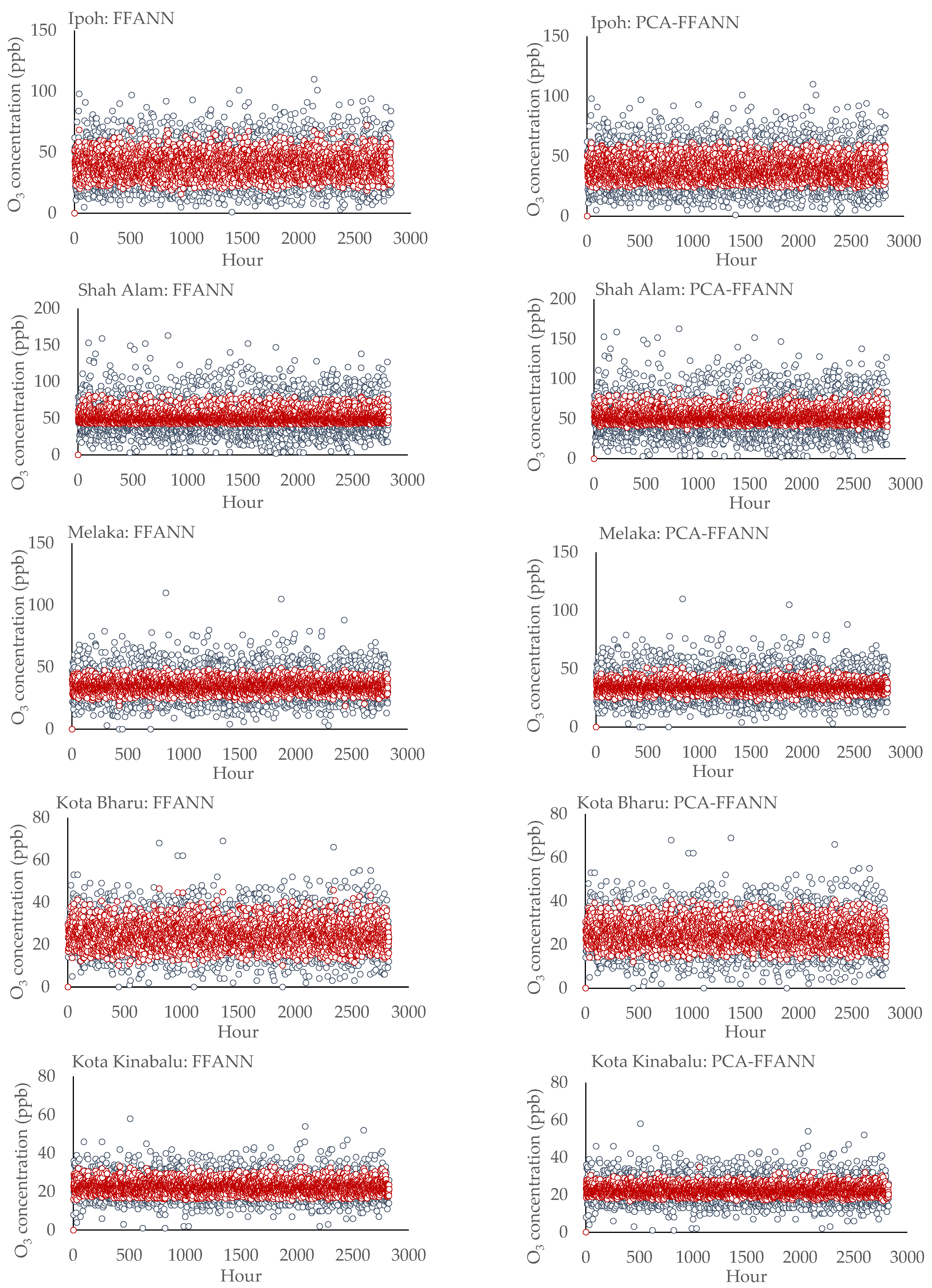
3.2.2. Artificial Neural Network (ANN) and Its Modification (PCA-FFANN)

The best performance indicated by the different number of neurons for the neural network analysis and the hybrid is shown in

Table 12. Model validation based on all parameters and PCA as inputs.

Location	Method	No. of Neuron	MAE	RMSE	IA	R2
Ipoh	FFANN	2	6.937	9.071	0.871	0.839
	PCA-FFANN	2	8.402	10.693	0.804	0.706
Shah Alam	FFANN	2	12.090	15.677	0.729	0.846
	PCA-FFANN	6	13.233	17.534	0.638	0.576
Melaka	FFANN	2	5.599	7.850	0.769	0.853
	PCA-FFANN	6	6.438	8.816	0.684	0.647
Kota Bharu	FFANN	2	2.449	3.519	0.940	0.949
	PCA-FFANN	4	3.708	4.918	0.870	0.771
Kota Kinabalu	FFANN	8	2.619	3.579	0.841	0.691
	PCA-FFANN	4	3.583	4.779	0.658	0.540

. Overall, FFANN performed very well compared to it modified-version model, i.e., PCA-FFANN. Basically, the predicted O₃ level using FFANN had low percentage of measured error (RMSE) compared to PCA-FFANN by around 20.3 percent. Furthermore, very good agreement between observed and predicted O₃ level was detected with FFFANN model due to very close value of the performance measures (PA, IA, and R²) to 1. This indicates that the prediction of maximum hour O₃ level were very close to the observed concentration of O₃. A number of researchers have been applying ANN for prediction of ambient air pollutants concentration. ANN was identified as one of the best models for PM₁₀ level prediction [31,53] and ground-level O₃ [24,25].

Comparatively, PCA-FFANN model performed moderately compared to FFANN in predicting O₃ level for all the areas. Principal components (PCs) were used as input to FFANN to reduce the dimension of a given data set, making the data set more approachable and computationally easier to handle, while preserving most patterns and trends. Modified model of FFANN (by using PCs as input to train and validate FFANN model) was expected to increase the accuracy of the model. A few studies have applied the modified FFANN model with PCA and had successfully increased the accuracy of the model in predicting PM₁₀ level [31,35] and ground-level O₃ concentration [25,36].

Graphical presentation of the predicted and observed O₃ level is presented in Figure 3. Generally, it can be seen that the predicted O₃ level using FFANN and PCA-FFANN was fitted with the range of the best fitted values by the model, which in this case were more distributed at the center of the observed data points. In addition, the range of O₃ level predicted by PCA-FFANN was observed to be smaller than the value predicted by FFANN, or, in other words, the range of the best fitted values was more narrowed compared to its non-modified model. However, better variation of the predicted values (FFANN was better than PCA-FFANN) was observed in Kota Bahru and Kota Kinabalu where the error was significantly small (Table 12) compared to other areas.

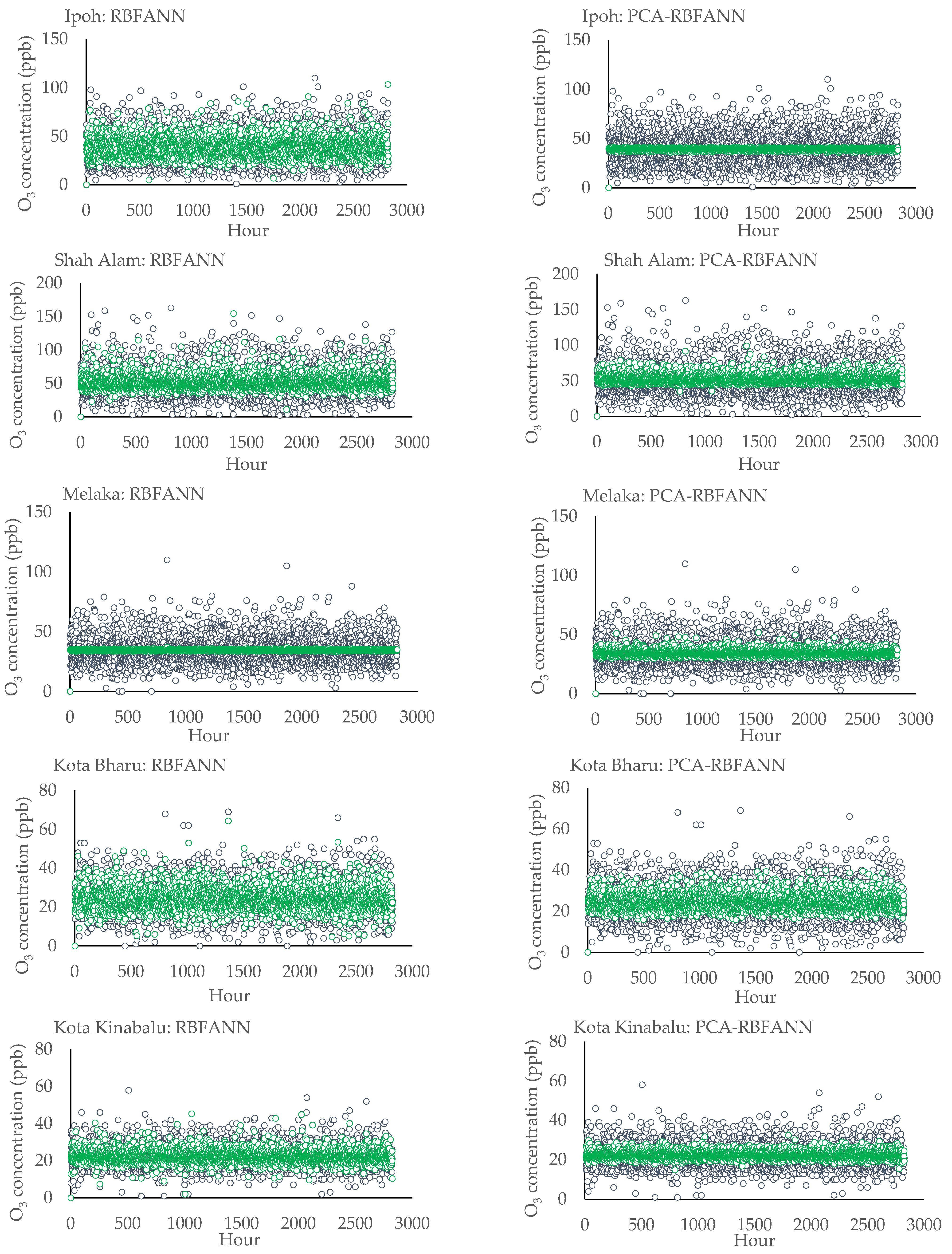
3.2.3. Radial Basis Functions (RBFANN) and Its Modification (PCA-RBFANN)

Table 13. Model validation based on all parameters and PCA as inputs.

Location	Method	Smoothness Function (σ)	MAE	RMSE	IA	R2
Ipoh	RBFANN	0.2	8.675	11.118	0.770	0.558
	PCA-RBFANN	0.1	9.148	11.640	0.746	0.587
Shah Alam	RBFANN	0.1	12.049	16.418	0.741	0.531
	PCA-RBFANN	0.1	13.941	18.422	0.567	0.539
Melaka	RBFANN	0.1	6.247	8.620	0.710	0.852
	PCA-RBFANN	0.1	7.577	9.977	0.506	0.649
Kota Bharu	RBFANN	0.1	3.173	4.579	0.899	0.775
	PCA-RBFANN	0.1	4.316	5.690	0.791	0.771
Kota Kinabalu	RBFANN	0.1	3.036	4.292	0.783	0.379
	PCA-RBFANN	0.1	3.774	4.990	0.587	0.483

shows the validation of models according to the best spread number for RBFANN and its modified model (PCA-RBFANN).

Generally, prediction of maximum O₃ level made by RBFANN was found out to be moderately good for all the study areas except for Melaka and Kota Bharu with the range of R² value from 0.531 to 0.852. Predicted O₃ levels using RBF neural network at these two cities were quite well-correlated with the value of R² of 0.852 and 0.775 for Melaka and Kota Bharu, respectively. Comparable findings were identified by a study conducted by Abdullah et al. [40], where RBFANN was used to predict PM₁₀ concentration in Pasir Gudang, Malaysia. The results showed that RBFANN model was able to explain 65.2% and 84.9% variance in the data during training and testing, respectively. Hence, it is proven that RBFANN is a promising nonlinear model which has high ability in representing the complexity and nonlinearity of ambient air pollutant concentration in the atmosphere.

The performance of RBFANN in predicting air pollutant level, if compared to another well-known neural network such as multi-layer perception (MLP), is known to be less accurate than other neural networks. This was supported by the findings from the study conducted by Kumar et al. [54] that compared RBF with MLP neural network for prediction of O₃ level in India. The results suggested that MLP had slightly better prediction of O₃ level with the range of RMSE value of 5.4 to 15.4 compared to RBF, with the range of 5.2 to 18.6.

Its modified version, PCA-RBFANN, performed less accurately than its basis model. However, noticeable improvement was observed on R² value for the Ipoh, Shah Alam, and Kota Kinabalu, where better goodness-of-fit measure of the predicted data to the regression line was detected. When a regression model accounts for more of the variance, the data points are closer to the regression line; hence, a better fitted model was witnessed.

Figure 4 shows the graphical exhibition of the predicted and observed O₃ level at all study areas. As a whole, inconsistent performances of the predicted values using RBFANN or PCA-RBFANN can be observed. For prediction using RBF neural network (RBFANN), all of the cities except for Melaka were detected to have wider range of the best fitted values compared to the predicted values by FFANN (Section 3.2.2). Predicted data points of O₃ level by PCA-RBFANN were observed to have narrower range of the best fitted values, especially in Ipoh and Kota Kinabalu. Oppositely, in Melaka, the predicted data points using RBFANN had a very constricted range of the best fitted values compared to its modified version (PCA-RBFANN).

3.3. Summary

Table 14. Summary of performance measures for the six prediction models.

Model	Performance Indicators
	MAE	RMSE	IA	R2
MLR	6.061	7.769	0.847	0.905
PCR	7.314	9.605	0.707	0.648
FFANN	5.939	7.937	0.830	0.877
PCA-FFANN	7.073	9.348	0.731	0.641
RBFANN	6.636	9.009	0.781	0.619
PCA-RBFANN	7.751	10.144	0.639	0.606

summarizes the performance of the six models used to predict the ground-level O₃ in Malaysia. Overall, MLR gives small error (6.061 and 7.769 for MAE and RMSE respectively) and offer most fitted data to the regression line, with the value of R² and IA close to 1. FFANN and RBFANN fitted the observed O₃ data points well but were slightly less accurate compared to MLR. Interestingly, all the unmodified models (MLR, FFANN, and RBFANN) significantly outperformed their modified version model (PCR, PCA-FFANN, and PCA-RBFANN). The sequence of model from the best fitted model to the least is as follows:

MLR > FFANN > RBFANN > PCR> PCA-FFANN > PCA-RBFANN

3.4. Deployment of the Best Selected Prediction Model of Ground-Level O₃

Deployment of the best-chosen model (MLR) was done in order to prove that the model was able to predict the maximum hour of O₃ concentration using different years of dataset.

Table 15. Performance measures of model verification for the five study areas.

Area/Performance	MAE	RMSE	IA	R2
Ipoh	8.030	10.815	0.759	0.887
Shah Alam	11.470	14.678	0.736	0.903
Melaka	9.263	12.331	0.744	0.952
Kota Bharu	2.363	3.208	0.951	0.944
Kota Kinabalu	2.447	3.197	0.928	0.866

shows the results of performance measures for the predicted O₃ level using MLR for the dataset of 2018. Small error measurement was detected, with ranges from 2.3 to 14.7 that resulted in small differences between the predicted and observed values of O₃ level. High accuracy of performance measures (IA and R²) indicates high agreement between the observed and predicted data points. Therefore, with this high agreement between the predicted data and the observed data, it was proven that the linear regression models can be used to predict the O₃ level at any year provided no to small significant change on the dataset variability. Good prediction model was able to be developed due to the long-term period (2003 to 2012), which was taken into account during development of model where 80% of the dataset was used for model development and the remaining was used to validate the performances of the model. Thus, deployment of MLR as the best selected model for predicting daytime O₃ concentration was considered effective.

4. Discussion

4.1. Performances of the Predictive Models (Basis Model)

Multiple Linear Regression predicted the maximum O₃ concentration better than other predictive models including the hybrid methods. High agreement between the observed and predicted values was witnessed with the calculated R² value > 0.8 for each study areas. MLR successfully modeled the relationship between the independent variables (previous O₃, NmHC, PM₁₀, SO₂, NO₂, and CO, wind speed, ambient temperature, humidity) and a dependent variable (O_3(t+1)), by fitting a linear equation to the observed data.

Multiple linear regression is one of the most widely used methods for predicting ozone concentrations with weather parameters and different atmospheric pollutants. In several studies conducted by Hassanzadeh et al. [11] and Barrero et al. [12], the connection between weather status and ozone concentration has been observed using this method. The best prediction equation for ozone and weather variables is found in Hassanzadeh et al. [11] using a multiple regression procedure. Barrero et al. [12] also show that the MLR allows maximum O₃ concentration to be predicted in city areas within several hours in advance. Banja et al. [13] applied multiple linear regression to predict the next day’s maximum ozone concentration for the first time in Tirana, Albania. The relationship between daily maximum ozone values and weather variables was investigated. MLR analysis has been performed to establish the relationship between the weather parameters and peak ozone concentration. It was found out that MLR performed well with the value of R² = 0.87. Abdullah et al. [55] investigated the variation of O₃ concentrations in Klang, Malaysia from 2012 to 2015. MLR model was developed and signifies that nitrogen oxides (NO), relative humidity (RH), NO₂, CO, wind speed, temperature, and sulphur dioxide (SO₂) are the significant predictors for O₃ concentration. The calculated value of R² for MLR is 0.810. Since MLR is a simple linear regression method that can easily be used to correlate other pollutants and weather parameters, it was abundantly used to model O₃ concentration. Hence, from the above mentioned studies, it can be proven that the maximum O₃ concentration was best explained by the simple linear regression.

FFANN gives good prediction for the maximum concentration of O₃; however, it was less accurate than MLR. The reduction percentage of R² for prediction model using FFANN and MLR was 8.2%, indicating that FFANN performed slightly less well than MLR in predicting maximum O₃ concentration in Malaysia. The main purpose of using neural artificial networks to model ozone is to capture the non-linear characteristics of the relationship overlooked by a conventional statistical technique (e.g., regression model) [54]. Even though ANN was known as a powerful predictive model, the main factor that influences the accuracy of the model was the associations of air pollutants and weather parameters. It was proven by the research conducted by Pawlak and Jaroslawski [25] that developed artificial neural network models for the prediction of the daily maximum hourly mean of surface ozone concentration for the next day at rural and urban locations in central Poland. The models were generated with six input variables: forecasted basic meteorological parameters and the maximum O₃ concentration recorded on the previous day and number of the month. The mean error (ME) value indicates a tendency to overestimate the predicted values by 4.8 µg/m³ for Belsk station and to underestimate the predicted values by 0.9 µg/m³ for Warsaw station. The analysis of days when the relative error value was >50% revealed that all predictions with extremely high relative error value were associated.

RBF gives the worst performance in predicting maximum O₃ concentration in Malaysia if compared to MLR and FFANN. Implementation of RBF model to predict air pollutant is still very recent. Abdullah et al. [47] trained and tested the nonlinear model, namely Radial Basis Function (RBF), to predict particulate matter (PM₁₀) concentration in an industrial area of Pasir Gudang, Johor, Malaysia. Daily observations of PM₁₀ concentration, meteorological factors (wind speed, ambient temperature, and relative humidity), and gaseous pollutants (SO₂, NO₂, and CO) from 2010 to 2014 were used. Results showed that RBF model was able to explain 65.2% (R² = 0.652) and 84.9% (R² = 0.849) variance in the data during training and testing, respectively. This finding was found to be similar to this study, where the prediction of maximum O₃ concentration using RBFANN in Malaysia was in the range of 0.38 to 0.85 (R²). Thus, it is proven that a nonlinear model has high potential in virtually representing the complexity and nonlinearity of O₃ in the atmosphere without any prior assumptions.

4.2. Performances of the Modified Models

Overall, the hybrid models of PCR, PCA-FFANN, and PCA-RBFANN performed worse than their basis models, i.e., MLR, FFANN, and RBFANN, respectively. The lesser accuracy of the models was mainly due to application of principal components (PCs) as an input to the modified models. Hair et al. [56] outlined that the variables needed to be included in the analysis of PCA should be ideally derived from past research studies or based on the judgement of other researchers. However, in Malaysia, there were very limited studies focusing on modeling of O₃ concentration for all regions of Malaysia. Most of the studies were performed at the Lembah Klang that was the most populous area in Malaysia [1,23,45].

As stated previously, the main propose of using principal components as input to the modified models was to reduce the dimension of the dataset, though, PCA as a dimension reduction methodology is applied without considering the association between the dependent variable (O₃ concentration) and independent variables (PM₁₀, CO, NO₂, SO₂, NmHC, UVB, humidity, wind speed, and temperature). Thus, PCA is termed as an unsupervised dimension reduction methodology [57]. The performance of the modified models was not as good as compared to its basis model alone because the principal components that were used as the input to this hybrid model is governed by cumulative of variance during grouping the factors. For example, the percentage of cumulative variances are 69% for Shah Alam, and 66% for Ipoh which is lower than 70% (from Table 7). This means that only 69% and 66% of the total variance is explained. Lower percentage of reliability will affect the performance of hybrid models that used the principal components as the input parameters. In detail, specifically take Shah Alam as an example. The first principal component (PC) contributed 32% (refer Table 8) of the total variance explained that the group of parameters were correlated to the O₃ concentration. However, for the second PC that was calculated 26% of the total variance was less explanatory for the target compared to the first factor. The third factor contributed only 10.6% of the total variance and it can be related to the target.

A few studies obtained similar findings as reported in this study. Ozbay et al. [58] also reported comparable findings with PCR showing significantly lower R² than MLR when studying the variation in O₃ at Dilovasi, Turkey. Elbayoumi et al. [57] also reported that the use of PCR does not increase the accuracy in predicting indoor PM₁₀ and PM_2.5 in the Gaza Strip (Palestine) compared with the use of MLR. For both of the studies, significant reductions of ranging from 20% to 30% have been reported [57,58]. Elbayoumi et al. [57] related the poor performance of PCR due to the fact that PCA is an unsupervised dimension reduction methodology.

Furthermore, PCs were usually not understandable. Most of supervised learning algorithms (for example logistic regression, tree-based algorithm, or neural network) can evaluate the importance of input features. These features are important as they help users to distinguish which data were further needed for exploration and features that might be beneficial or worth more [58]. These features, when combined with the machine learning algorithm, are expected to enhance the accuracy of the model [40,41]. Balogun and Tella [40] reported that the input feature of Random Forest when combined with regression contributed to higher accuracy model with high of R² (0.97). However, when applying principal components as the input, reduction of predictive tools can be expected since it is done in such a way that the principal components are orthogonal and have the largest possible variances which did not truly interpret the actual situation.

All the issues in applying PCA that were highlighted above might be the reasons that lessen the performances of the modified models in predicting the daytime concentration of O₃ in Malaysia.

5. Conclusions

Six models (MLR, FFANN, RBFANN, and their modified models, namely PCR, PCA-FFANN, and PCA-RBFANN) were developed to predict daytime O₃ level at five specified study areas. Out of six models, MLR outperformed other methods with highest accuracy prediction for all study areas. This indicates that the daytime O₃ level in major urban areas in Malaysia is best described using linear regression. This might be due to very limited or less extreme concentration observed in the O₃ dataset; hence, a linear regression model is applicable to predict daytime O₃ concentration for most urban areas in Malaysia.

For nonlinear models, FFANN gives better prediction compared to RBFANN. The differences in the basis function of the two machine algorithms might be the reason for the worse predictions made by RBFANN. RBFANN has localized basis functions (e.g., Gaussian) whereas FFANN has global basis functions (sigmoid). Since this study predicted O₃ level at the greatest band of solar intensity, sigmoid basis function was more relevant in fitting the dataset.

On the other hand, all the modified models show underperform prediction compared to the unmodified models. The main reason for this reduced efficiency was the input to the modified models. In the modified models, the selected principal components from the output of Principal Component Analysis (PCA) were used as input. These inputs were selected based on the high factor loading and eigenvalues (>1) for each principal component. However, this selection of inputs leads to multidimensional issues and feature redundancy that lead to a less effective model.

References

1. Awang, N.R.; Elbayoumi, M.; Ramli, N.A.; Yahaya, A.S. Diurnal variations of ground-level ozone in three port cities in Malaysia. Air Qual. Atmos. Health 2015, 9, 25–39. [Google Scholar] [CrossRef]
2. Yin, Y.; Fook, S.; Glasow, R.V. The influence of meteorological factors and biomass burning on surface ozone concentrations at Tanah Rata, Malaysia. Atmos. Environ. 2013, 70, 435–446. [Google Scholar]
3. Tan, K.C.; Lim, H.S.; Zubir, M.; Jafri, M. Prediction of column ozone concentrations using multiple regression analysis and principal component analysis techniques: A case study in peninsular Malaysia. Atmos. Pollut. Res. 2016, 7, 533–546. [Google Scholar] [CrossRef]
4. Faris, H.; Alkasassbeh, M.; Rodan, A. Artificial neural networks for surface ozone prediction: Models and analysis. Pol. J. Environ. Stud. 2014, 23, 341–348. [Google Scholar]
5. Eum, J.; Kim, H. Effects on Air Pollution in Assaults: Finding from South Korea. Sustainability 2021, 13, 11545. [Google Scholar] [CrossRef]
6. Department of Environment Malaysia. Environmental Quality Report 2018; Department of Environment Malaysia: Selangor, Malaysia, 2019; pp. 142–156. [Google Scholar]
7. Teixeira, E.C.; de Santana, E.R.; Wiegand, F.; Fachel, J. Measurement of surface ozone and its precursors in an urban area in South Brazil. Atmos. Environ. 2009, 43, 2213–2220. [Google Scholar] [CrossRef]
8. Al-Shammari, E.T. Towards an accurate ground-level ozone prediction. Int. J. Electr. Comput. Eng. 2018, 8, 1131–1139. [Google Scholar]
9. Verma, N.; Kumari, S.; Lakhani, A.; Kumari, K.M. 24 Hour Advance Forecast of Surface Ozone Using Linear and Non-Linear Models at a Semi-Urban Site of Indo-Gangetic Plain. Int. J. Environ. Sci. Nat. Res. 2019, 18, 555982. [Google Scholar]
10. Verma, N.; Satsangi, A.; Lakhani, A.; Kumari, K.M. Prediction of Ground level Ozone concentration in Ambient Air using Multiple Regression Analysis. J. Chem. Biol. Phys. Sci. 2015, 5, 3685–3696. [Google Scholar]
11. Hassanzadeh, S.; Hosseinibalam, F.; Omidvari, M. Statistical methods and regression analysis of stratospheric ozone and meteorological variables in Isfahan. Phys. A Stat. Mech. Appl. 2008, 387, 2317–2327. [Google Scholar] [CrossRef]
12. Barrero, M.A.; Grimalt, J.O.; Canto’n, L.M. Prediction of daily ozone concentration maxima in the urban atmosphere. Chemometr. Intell. Lab. Syst. 2006, 80, 67–76. [Google Scholar] [CrossRef]
13. Banja, M.; Papanastasiou, D.K.; Poupkou, A.; Melas, D. Atmospheric Pollution Research Development of a short–term ozone prediction tool in Tirana area based on meteorological variables. Atmos. Pollut. Res. 2012, 3, 32–38. [Google Scholar] [CrossRef] [Green Version]
14. Allu, S.K.; Srinivasan, S.; Maddala, R.K.; Reddy, A.; Anupoju, G.R. Seasonal ground level ozone prediction using multiple linear regression (MLR) model. Model. Earth Syst. Environ. 2020, 6, 1981–1989. [Google Scholar] [CrossRef]
15. Azmi, S.T.; Latif, M.T.; Jemain, A.A. Trend and status of air quality at three different monitoring stations in the Klang Valley, Malaysia. Air Qual. Atmos. Health 2010, 3, 53–64. [Google Scholar] [CrossRef] [Green Version]
16. Awang, M.B.; Jaafar, A.B.; Abdullah, A.M.; Ismail, M.B.; Hassan, M.N.; Abdullah, R.; Johan, S.; Noor, H. Air quality in Malaysia: Impacts, management issues and future challenges. Respirology 2000, 5, 183–196. [Google Scholar] [CrossRef] [PubMed]
17. Ismail, M.; Abdullah, S.; Yuen, S.F.; Ghazali, N.A. A ten-year investigation on ozone and it precursors at Kemaman, Terengganu, Malaysia. EnvironmentAsia 2016, 9, 1–8. [Google Scholar]
18. Ghazali, N.A.; Ramli, N.A.; Yahaya, A.S.; Yusof, N.F.F.M.; Sansuddin, N.; Al Madhoun, W.A. Transformation of nitrogen dioxide into ozone and prediction of ozone concentrations using multiple linear regression techniques. Environ. Monit. Assess. 2010, 165, 475–489. [Google Scholar] [CrossRef]
19. Tong, W. Chapter 5-machine learning for spatiotemporal big data in air pollution. In Spatiotemporal Analysis of Air Pollution and its Application in Public Health; Li, L., Zhou, X., Tong, W., Eds.; Elsevier: Amsterdam, The Netherlands, 2020. [Google Scholar]
20. Dou, J.; Yunus, A.P.; Tien Bui, D.; Merghadi, A.; Sahana, M.; Zhu, Z.; Chen, C.-W.; Khosravi, K.; Yang, Y.; Pham, B.T. Assessment of advanced random forest and decision tree algorithms for modeling rainfall-induced landslide susceptibility in the Izu-Oshima Volcanic Island, Japan. Sci. Total Environ. 2019, 662, 332–346. [Google Scholar] [CrossRef]
21. Ma, J.; Ding, Y.; Cheng, J.C.P.; Jiang, F.; Tan, Y.; Gan, V.J.L.; Wan, Z. Identification of high impact factors of air quality on a national scale using big data and machine learning techniques. J. Clean. Prod. 2020, 244, 118955. [Google Scholar] [CrossRef]
22. Li, R.; Cui, L.; Meng, Y.; Zhao, Y.; Fu, H. Satellite-based prediction of daily SO2 exposure across China using a high-quality random forest-spatiotemporal Kriging (RF-STK) model for health risk assessment. Atmos. Environ. 2019, 208, 10–19. [Google Scholar] [CrossRef]
23. Al-Alawi, S.M.; Abdul-Wahab, S.A.; Bakheit, C.S. Combining principal component regression and artificial neural networks for more accurate predictions of ground-level ozone. Environ. Model. Softw. 2008, 23, 396–403. [Google Scholar] [CrossRef]
24. Padma, K.; Samuel Selvaraj, R.; Arputharaj, S.; Milton Boaz, B. Improved Artificial Neural Network Performance on Surface Ozone Prediction Using Principal Component Analysis. Int. J. Curr. Res. Rev. 2018, 6, 1–6. [Google Scholar]
25. Pawlak, I.; Jarosławski, J. Forecasting of surface ozone concentration by using artificial neural networks in rural and urban areas in central Poland. Atmosphere 2019, 10, 52. [Google Scholar] [CrossRef] [Green Version]
26. Aljanabi, M.; Shkoukani, M.; Hijjawi, M. Ground-level Ozone Prediction Using Machine Learning Techniques: A Case Ground-level Ozone Prediction Using Machine Learning Techniques: A Case Study in Amman, Jordan. Int. J. Autom. Comput. 2020, 17, 667–677. [Google Scholar] [CrossRef]
27. Castro, M.; Pires, J.C.M. Decision support tool to improve the spatial distribution of air quality monitoring sites. Atmos. Pollut. Res. 2019, 10, 827–834. [Google Scholar] [CrossRef]
28. Zhang, Y.-F.; Fitch, P.; Thorburn, P.J. Predicting the Trend of Dissolved Oxygen Based on the kPCA-RNN Model. Water 2020, 12, 585. [Google Scholar] [CrossRef] [Green Version]
29. Banadkooki, F.B.; Ehteram, M.; Ahmed, A.N.; Fai, C.M.; Afan, H.A.; Ridwam, W.M.; Sefelnasr, A.; El-Shafie, A. Precipitation forecasting using multilayer neural Network and support vector machine optimization based on flow regime algorithm taking into Account uncertainties of soft computing models. Sustainability 2019, 11, 6681. [Google Scholar] [CrossRef] [Green Version]
30. Ehteram, M.; Ahmed, A.N.; Ling, L.; Fai, C.M.; Latif, S.D.; Afan, H.A.; Banadkooki, F.B.; El-Shafie, A. Pipeline scour rates prediction-based model utilizing a multilayer perceptron colliding body algorithm. Water 2020, 12, 902. [Google Scholar] [CrossRef] [Green Version]
31. Ul–Saufie, A.Z.; Yahaya, A.S.; Ramli, N.A.; Rosaida, N.; Hamid, H.A. Future daily PM10 concentrations prediction by combining regression models and feedforward backpropagation models with principle component analysis (PCA). Atmos. Environ. 2013, 77, 621–630. [Google Scholar] [CrossRef]
32. Hashim, N.I.M.; Noor, N.M.; Annas, S. Influence of meteorological factors on variations of particulate matter (PM10) concentration during haze episodes in Malaysia. In AIP Conference Proceedings; AIP Publishing LLC: New York, NY, USA, 2018; Volume 2045. [Google Scholar]
33. Thupeng, W.M.; Mothupi, T.; Mokgweetsi, B.; Mashabe, B.; Sediadie, T. A Principal Component Regression Model, For Forecasting Daily Peak Ambient Ground Level Ozone Concentrations, in The Presence Of Multicollinearity Amongst Precursor Air Pollutants And Local Meteorological Conditions: A Case Study Of Maun. Int. J. Appl. Math. Stat. Sci. 2018, 7, 1–12. [Google Scholar]
34. Ismail, M.; Abdullah, S.; Jaafar, A.D.; Ibrahim, T.A.E.; Shukor, M.S.M. Statistical modeling approaches for PM10 forecasting at industrial areas of Malaysia. AIP Conf. Proc. 2018, 2020, 020044. [Google Scholar]
35. Taspinar, F. Improving artificial neural network model predictions of daily average PM10 concentrations by applying principle component analysis and implementing seasonal models. J. Air Waste Manag. Assoc. 2015, 65, 800–809. [Google Scholar] [CrossRef] [PubMed]
36. Bekesiene, S.; Meidute-kavaliauskiene, I. Accurate Prediction of Concentration Changes in Ozone as an Air Pollutant by Multiple Linear Regression and Artificial Neural Networks. Mathematics 2021, 9, 356. [Google Scholar] [CrossRef]
37. Lu, W.-Z.; Wang, W.-J.; Wang, X.-K.; Yan, S.-H.; Lam, J.C. Potential assessment of a neural model PCA/RBF approach for forecasting pollution trends in Mongkok urban air, Hong Kong. Environ. Res. 2004, 96, 79–87. [Google Scholar] [CrossRef] [PubMed]
38. Tikhamarine; Yazid; Souag-Gamane, D.; Najah Ahmed, A.; Kisi, O.; El-Shafie, A. Improving artificial intelligence models accuracy for monthly streamflow forecasting using grey Wolf optimization (GWO) algorithm. J. Hydrol. 2020, 582, 124435. [Google Scholar] [CrossRef]
39. Abobakr Yahya, A.S.; Ahmed, A.N.; Othman, F.B.; Ibrahim, R.K.; Afan, H.A.; El-Shafie, A.; Fai, C.M.; Hossain, M.S.; Ehteram, M.; Elshafie, A. Water quality prediction model based support vector machine model for ungauged river catchment under dual scenarios. Water 2019, 11, 1231. [Google Scholar] [CrossRef] [Green Version]
40. Balogun, A.-L.; Tella, A. Modelling and investigating the impacts of climatic variables on ozone concentration in Malaysia using correlation analysis with random forest, decision tree regression, linear regression, and support vector regression. Chemosphere 2022, 299, 134250. [Google Scholar] [CrossRef]
41. Ayman, Y.; AlDahoul, N.; Birima, A.H.; Ahmed, A.N.; Sherif, M.; Sefelnasr, A.; Allawi, M.F.; Elshafie, A. Comprehensive comparison of various machine learning algorithms for short-term ozone concentration prediction. Alex. Eng. J. 2022, 61, 4607–4622. [Google Scholar]
42. Kaiser, H.F. An index of factorial simplicity. Psychometrika 1974, 39, 31–36. [Google Scholar] [CrossRef]
43. Brūmelis, G.; Brown, D.H.; Nikodemus, O.; Tjarve, D. The monitoring and risk assessment of Zn deposition around metal smelter in Latvia. Environ. Monit. Assess. 1999, 58, 201–212. [Google Scholar] [CrossRef]
44. Juahir, H.; Zain, S.M.; Yusoff, M.K.; Tengku Hanidza, T.I.; Mohd Armi, A.S.; Toriman, M.E.; Mokhtar, M. Spatial water quality assessment of Langat River Basin (Malaysia) using environmetric techniques. Environ. Monit. Assess. 2011, 173, 625–641. [Google Scholar] [CrossRef] [Green Version]
45. Azid, A.; Juahir, H.; Latif, M.T.; Zain, S.M. Feed-Forward Artificial Neural Network Model for Air Pollutant Index Prediction in the Southern Region of Peninsular Malaysia. J. Environ. Prot. Sci. 2013, 4, 40509. [Google Scholar] [CrossRef]
46. Azid, A.; Juahir, H.; Toriman, M.E.; Kamarudin, M.K.A.; Saudi, A.S.M.; Hasnam, C.N.C.; Aziz, N.A.A.; Azaman, F.; Latif, M.T.; Zainuddin, S.F.M.; et al. Prediction of the Level of Air Pollution Using Principal Component Analysis and Artificial Neural Network Techniques: A Case Study in Malaysia. Water Air Soil. Pollut. 2014, 225, 2063. [Google Scholar] [CrossRef]
47. Abdullah, S.; Mohd Napi, N.N.L.; Ahmed, A.N.; Wan Mansor, W.N.; Abu Mansor, A.; Ismail, M.; Abdullah, A.M.; Ramly, Z.T.A. Development of Multiple Linear Regression for Particulate Matter (PM10) Forecasting during Episodic Transboundary Haze Event in Malaysia. Atmosphere 2020, 11, 289. [Google Scholar] [CrossRef] [Green Version]
48. Sun, G.; Hoff, S.J.; Zelle, B.C.; Nelson, M.A. Development and Comparison of Backpropagation and Generalized Regression Neural Network Models to Predict Diurnal and Seasonal Gas and PM10 Concentrations and Emissions from Swine Buildings. Trans. Am. Soc. Agric. Biol. Eng. 2008, 51, 685–694. [Google Scholar]
49. Gvozdic, V.; Kovac-Andric, E.; Brana, J. Influence of meteorological factors NO2, SO2, CO and PM10 on the concentration of O3 in the urban atmosphere of Eastern Croatia. Environ. Model. Assess. 2011, 16, 491–501. [Google Scholar] [CrossRef]
50. Ahmat, H.; Yahaya, A.S.; Ramli, N.A. PM10 Analysis for Three Industrialized Areas using Extreme Value. Sains Malays. 2015, 44, 175–185. [Google Scholar] [CrossRef]
51. Ghazali, N.A.; Yahaya, A.S.; Mokhtar, M.I.Z. Predicting Ozone Concentrations Levels Using Probability Distributions. ARPN J. Eng. Appl. Sci. 2014, 9, 2089–2094. [Google Scholar]
52. Ul-Saufie, A.Z.; Yahaya, A.S.; Ramli, N.A.; Hamid, H.A. Performance of Multiple Linear Regression Model for Longterm PM10 Concentration Prediction based on Gasesous and Meteorological Parameters. J. Appl. Sci. 2012, 12, 1488–1494. [Google Scholar] [CrossRef]
53. Abdullah, S.; Ismail, M.; Ahmed, A.N. Multi-layer perceptron model for air quality prediction. Malays. J. Math. Sci. 2019, 13, 85–95. [Google Scholar]
54. Kumar, N.; Middey, A.; Rao, P.S. Prediction and examination of seasonal variation of ozone with meteorological parameter through artificial neural network at NEERI, Nagpur, India. Urban Clim. 2017, 20, 148–167. [Google Scholar] [CrossRef]
55. Abdullah, A.; Ismail, M.; Fong, S.Y. Multiple Linear Regression (MLR) Models for Long Term PM10 Concentration Forecasting During Different Monsoon Seasons. J. Sustain. Sci. Manag. 2017, 12, 60–69. [Google Scholar]
56. Hair, J.F.; Anderson, R.E.; Tatham, R.L.; Black, W.C. Multivariate Data Analysis with Reading, 4th ed.; Prentice-Hall: Englewood Cliffs, NJ, USA, 1995. [Google Scholar]
57. Elbayoumi, M.; Yahaya, A.S.; Ramli, N.A.; Noor Md Yusof, N.F.F.; Al Madhoun, W.; Ul-Saufie, A.Z. Multivariate methods for indoor PM10 and PM2.5 modelling in naturally ventilated schools buildings. Atmos. Environ. 2014, 94, 11–21. [Google Scholar] [CrossRef]
58. Ozbay, B.; Keskin, G.A.; Dogruparmak, S.C.; Ayberk, S. Multivariate methodsforground level ozone modeling. Atmos. Res. 2011, 102, 57–65. [Google Scholar] [CrossRef]
Figure 1. Location of the five selected air quality monitoring stations in Malaysia.
Sustainability 14 07936 g001
Figure 2. Observed versus predicted values of ground-level O3 concentration using MLR and PCR. The blue marker is the observed value and the brown marker shows the predicted values.
Sustainability 14 07936 g002
Figure 3. Observed versus predicted ground-level O3 concentration using FFANN and PCA-FFANN. The blue marker is the observed values and the red marker shows the predicted values.
Sustainability 14 07936 g003
Figure 4. Observed versus predicted ground-level O3 using RBFANN and PCA-RBFANN. The blue marker is the observed values and the green marker shows the predicted values.
Sustainability 14 07936 g004