A TLBO-Tuned Neural Processor for Predicting Heating Load in Residential Buildings

Abstract

Recent studies have witnessed remarkable merits of metaheuristic algorithms in optimization problems. Due to the significance of the early analysis of the thermal load in energy-efficient buildings, this work introduces and compares four novel optimizer techniques—the firefly algorithm (FA), optics-inspired optimization (OIO), shuffled complex evolution (SCE), and teaching–learning-based optimization (TLBO)—for an accurate prediction of the heating load (HL). The models are applied to a multilayer perceptron (MLP) neural network to surmount its computational shortcomings. The models are fed by a literature-based dataset obtained for residential buildings. The results revealed that all models used are capable of properly analyzing and predicting the HL pattern. A comparison between them, however, showed that the TLBO-MLP with the coefficients of determination 0.9610 vs. 0.9438, 0.9373, and 0.9556 (respectively, for FA-MLP, OIO-MLP, and SCE-MLP) and the root mean square error of 2.1103 vs. 2.5456, 2.7099, and 2.2774 presents the most reliable approximation of the HL. It also surpassed several methods used in previous studies. Thus, the developed TLBO-MLP can be a beneficial model for subsequent practical applications.

1. Introduction

Heating, ventilating, and air conditioning (HVAC) systems [1] are an important component of new buildings, because their task is to adjust indoor air conditions. On the other hand, due to the growing tendency of people dwelling in energy-efficient buildings, having a reliable foreknowledge of the amount of required thermal loads can give insights for the appropriate selection of HVAC systems. Until now, many attempts have focused on optimizing HVAC systems through various mathematical and analytical methods [2,3,4]. At the same time, recent research has suggested the benefit of using machine-learning techniques (i.e., inverse modeling) for predicting the energy performance of buildings [5].

From a general perspective, engineers have recently benefited from advancements in computational and programming sciences, which have led to the development of new methodologies for various purposes [6,7,8]. Facilitating the simulations of real-world events has been a primary objective for this purpose [8,9,10]. A diversity of solutions have given experts the chance to choose the most appropriate approach (e.g., numerical [11,12], experimental [13,14], empirical [15,16], etc.) with respect to the unsolved problem. Machine learning, however, due to its advantages, has emerged as a potential substitute to many of these traditional methods. A wide variety of machine learning tools have solved complex issues with desirable accuracy [17,18,19].

An artificial neural network (ANN) [20] represents a robust intelligent processor for modeling objectives in various scientific fields [21,22,23]. Composed of several layers and neural processors, a multi-layer perceptron (MLP) [24] is known as a widely used type of ANN. These processors have been profitably applied for energy-related simulations [25,26,27]. An MLP maps the association of a dependent parameter with independent factors. In each processor of the MLP, called a neuron, a weight is assigned to each dependent parameter. The summation of the resultant value with a bias term will then be the input of an activation function. This method is implemented by the subsequent neurons to have a forward movement. This is why the MLP is categorized as a feed-forward tool [28].

Ren et al. [29] proposed using an ANN for the heat loss prediction of buildings, and their results showed good agreement with analytical approaches. Mohammadhassani et al. [30] showed the superiority of this model in forecasting the strain of a tie section within beams made of concrete. Sadeghi et al. [31] used an MLP for predicting the cooling load (CL) and heating load (HL) of a residential building. They also benefited from a sensitivity analysis that found the best response of the networks. Sholahudin and Han [32] employed a simplified dynamic version of an ANN associated with the Taguchi technique for the efficient prediction of HL in an HVAC system. More studies about the application of ANNs in energy modeling can be found in earlier literature [33,34,35]. Furthermore, analogous machine-learning models such as the fuzzy network [36], random forest [37], and support vector-based models [38] have presented valuable evaluations of energy-based issues.

Apart from well-known intelligent predictors, metaheuristic science has received growing consideration in many fields [39,40], particularly energy analysis and HVAC systems [41,42]. Katebi et al. [43] attained the optimal condition of a wavelet-based linear quadratic regulator using metaheuristic methods. Martin et al. [44] used a metaheuristic technique along with sensitivity analysis for parameter adjustment in order to calibrate the HVAC sub-system component. Likewise, Bamdad Masouleh [45] employed two types of ant colony optimization (for continuous and mixed variables) for building energy optimization. The superiority of the proposed models was also demonstrated in comparison to a number of benchmarks.

The suitable applicability of these algorithms has frequently been shown for optimizing machine-learning models [46,47,48]. Zhou et al. [49] compared the competency of particle swarm optimization (PSO) and artificial bee colony (ABC) applied to an ANN for estimating the HL and CL. An approximately 22 to 24% accuracy increase demonstrated the efficiency of both algorithms, and the PSO performed more effectively. Bui et al. [50] employed an electromagnetism-based firefly scheme for optimizing the ANN in approximating energy consumption. It was shown that their hybrid method was more accurate than a regular ANN. Moayedi et al. [51] tested the effectiveness of two optimizers, namely gray wolf optimization (GWO) and the grasshopper optimization algorithm (GOA), synthesized with an ANN for the HL estimation of a residential building. The obtained accuracies showed that utilizing these algorithms results in reducing the prediction error from 2.9859 to 2.4459 and 2.2899, respectively.

It has been discussed that metaheuristic algorithms perform such optimizations through the prevailing computational drawbacks, such as local minima [52] and dimension danger [53]. In general, it is obvious that allowing these algorithms to supervise the training of intelligent models would result in powerful prediction models for any purpose [54,55]. On the other hand, considering the wide variety of optimization techniques, conducting comparative studies for the new generation of a metaheuristic family is of high importance.

For the problem of energy performance analysis, discovering a reliable model for thermal load modeling can be beneficial from an environmental and economical point of view. It is for this reason that our research investigates the suitability of four novel metaheuristic optimizers, namely the firefly algorithm (FA), optics-inspired optimization (OIO), shuffled complex evolution (SCE), and teaching–learning-based optimization (TLBO), for the problem of HL estimation. One motivation for considering TLBO is the excellent performance of this strategy in appraising the CL by Zhou et al. [56]. The algorithms are synthesized with an ANN to adjust computational parameters. The hybrid ensembles are compared to identify the most robust technique that can be used for practical estimations of HL from the building characteristics.

2. Materials and Methods

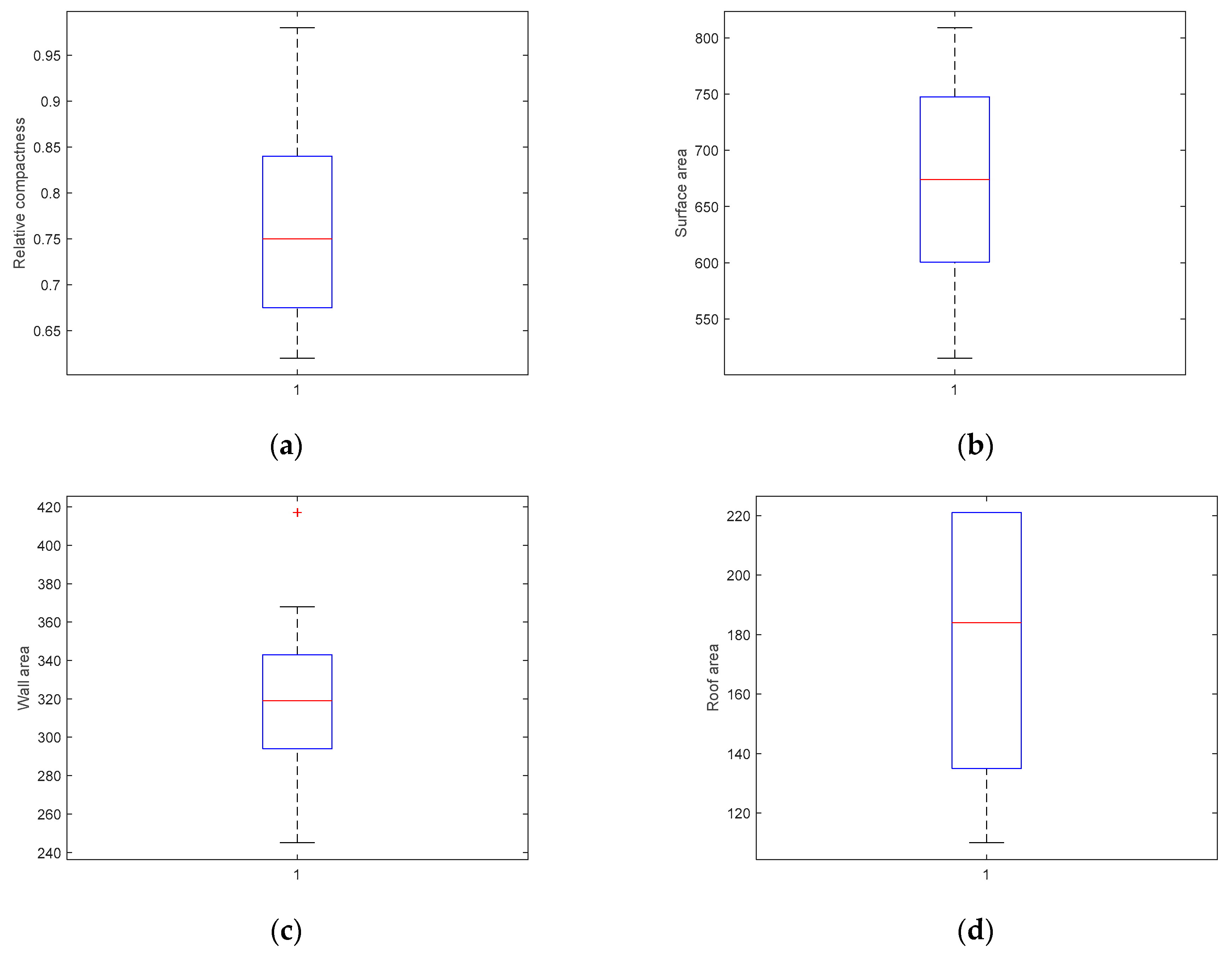
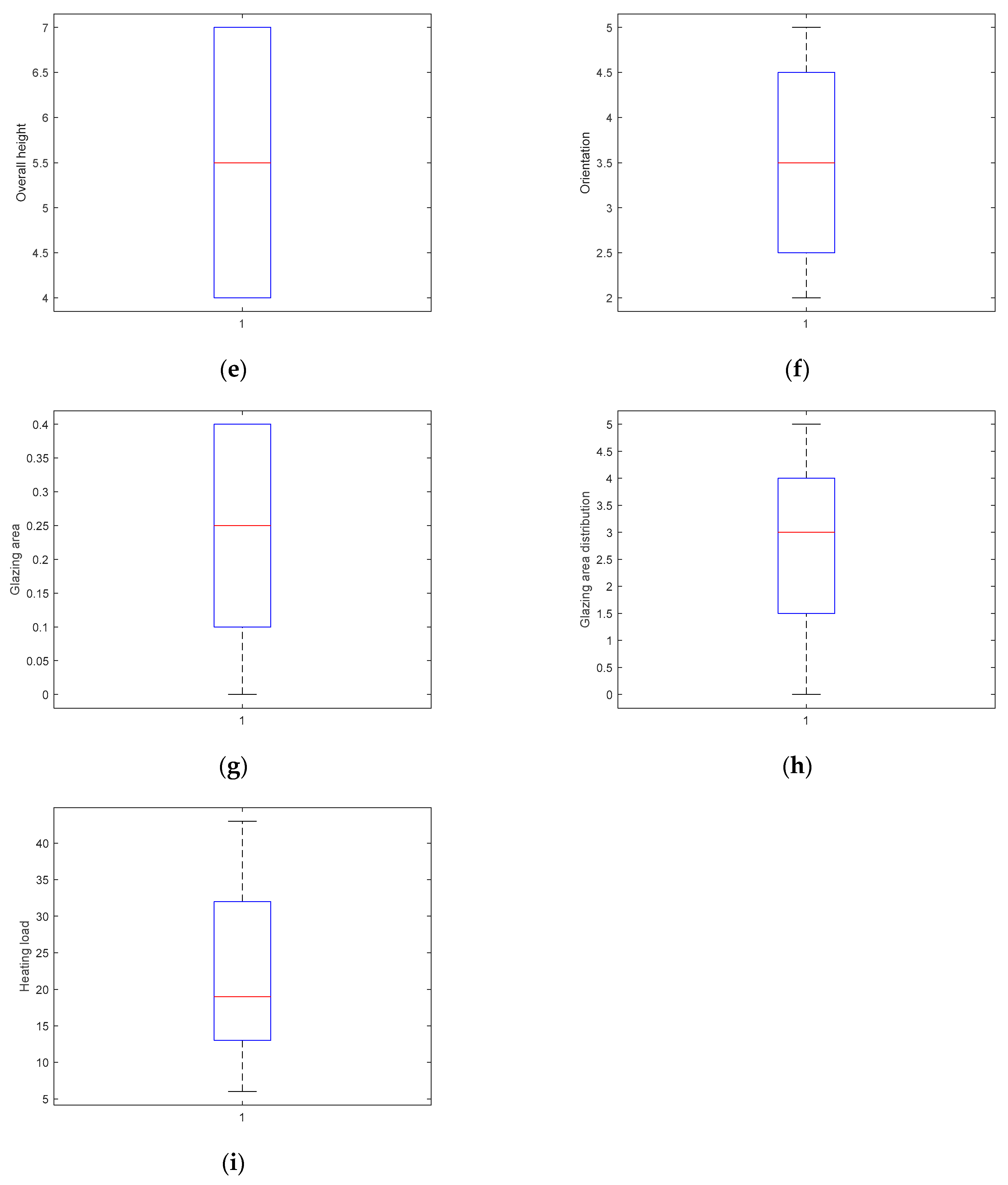
2.1. Data Provision

In order to approximate a parameter, the relationship between the parameter and influential factors should be analyzed. Therefore, providing a valid dataset is a necessary task. In this study, 768 thermal load conditions are used for training and testing the models. Tsanas and Xifara [57] implemented a vast analysis of HL and CL for different residential buildings. Their efforts resulted in gathering a widely used dataset, which can be accessed at http://archive.ics.uci.edu/ml/datasets/Energy+efficiency (accessed on 4 October 2021).

The HL and CL are the output parameters (i.e., dependent factors) considered to be affected by eight influential parameters (i.e., independent factors), namely roof area (RA), relative compactness (RC), glazing area (GA), wall area (WA), overall height (OH), surface area (SA), orientation (OR), and glazing area distribution (GAD). Figure 1 depicts a box plot of the HL and input factors.

As mentioned, a total of 768 samples were provided. By a random sampling, 614 records (i.e., 80% of 768) were selected and assigned as training data to be used for HL pattern analysis, and a residual 154 records (i.e., 20% of 768) were considered as testing data to assess the prediction efficiency of the models.

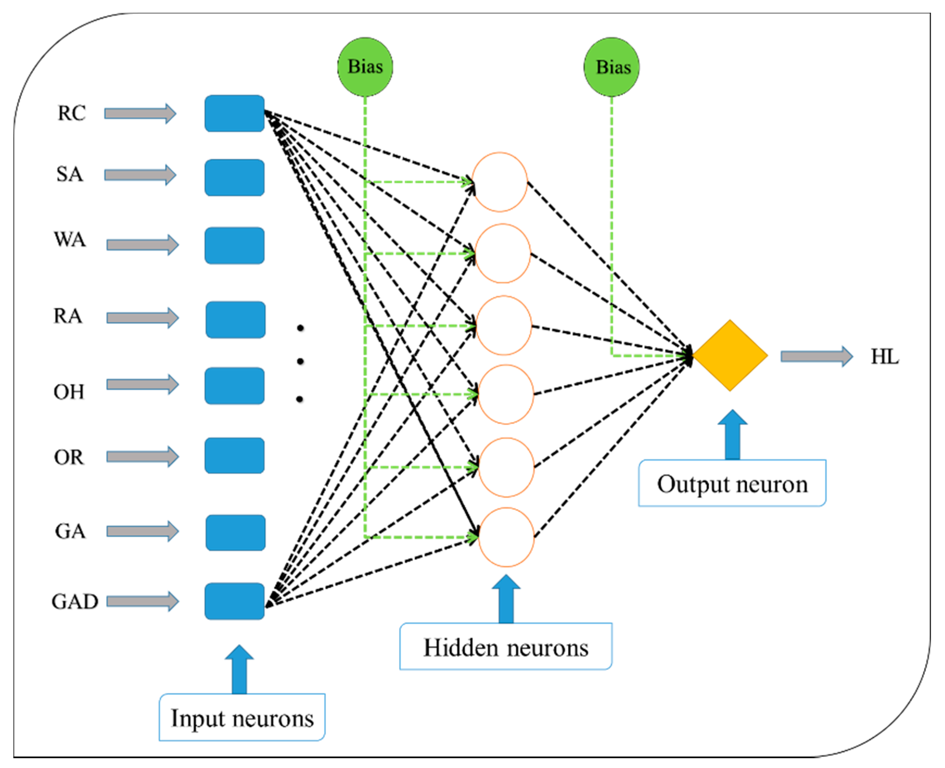
2.2. Methodology

As explained, in response to the drawbacks in the conventional neural network, this study investigates the effect of four novel optimizers, namely FA, OIO, SCE, and TLBO, on the performance of an ANN. Specifically, these algorithms are search schemes that aim to find the best hyperparameters of the ANN to be replaced with those suggested by typical learning rules (Levenberg–Marquardt [58] and backpropagation [59]).

The flashing behavior of fireflies is the basis of the FA algorithm. This nature-inspired method was first suggested by Yang [60] in 2008. In this strategy, there are two significant parameters, namely the intensity variation of light and the attractiveness formulation. As a maxim, the members of the FA are attracted to each other regardless of whether they are male or female. Further, the suitability of candidate solutions is determined by the brightness of the fireflies; the brighter members create more attractiveness. The reader may refer to earlier studies for mathematical details of the FA [61,62,63].

Kashan [64] designed the OIO as a capable physics-based search scheme. This algorithm draws on the relationships between the light, mirror, and pictures in a virtual space. Specifically, a number of light points are first generated as the population. They then produce an artificial image in the problem space with the help of a mirror. Updating the position of the generated image is the essential task of the OIO for adjusting the solutions. More information about this algorithm is available in previous literature [65,66,67].

The name SCE implies a well-known optimizer developed by Duan et al. [68]. The essence of the SCE is synthesizing four theories, namely controlled random search, genetic algorithm, complex shuffling, and the Nelder–Mead (downhill simplex) method [69]. Like many other optimization techniques, the algorithm begins by producing a scattered population and ends with meeting a satisfaction criterion. Among these steps, the complexes of the individuals are partitioned, evolved, and shuffled to implement optimization. For more detailed information about the algorithms, related studies are recommended [70,71,72].

Mimicking the interaction of the tutor and pupil in class, the TLBO was introduced by Rao et al. [73] in 2011 as a swarm-based metaheuristic algorithm. In this model, the teacher tries to establish the highest cooperation among students. As in reality, the teacher assesses the students by giving exams, and the teacher would like the students to achieve their maximum learning capability. In this model, a difference vector (i.e., differences between two individuals) is calculated, and the students aim to update themselves accordingly. The TLBO is better detailed in studies such as [74,75].

3. Results and Discussion

According to Section 1, this paper investigates the capability of four novel optimizations of a neural network for HL approximation. This objective is fulfilled by synthesizing the algorithms with an MLP neural network. Utilizing a specific search scheme, each algorithm tries to find the most appropriate values for the computational weights (and biases) belonging to the MLP.

As is known, the structure of the MLP relies on a hidden layer’s size and the contained neurons therein. Thus, these parameters need to be optimized first. One hidden layer is considered for the MLP, as many studies have proved the competence of one hidden layer for modeling complex phenomena [76,77]. However, a trial-and-error practice was used to identify the best number for the hidden neurons. The results showed that among the tested structures (where the middle layer contains 1, 2, 3, …, 10 neurons), 8 × 6 × 1 gives the most promising performance. Figure 2 shows the MLP used.

3.1. Accuracy Indicators

The root mean square error (RMSE) and mean absolute error (MAE) are defined for measuring the learning and prediction errors. Equations (1) and (2) give the RMSE and MAE formulation. Further, Equation (3) defines the coefficient of determination (R²) that is used to calculate the compatibility between the measured and forecasted HLs:

$$\mathrm{MAE}=\frac{1}{U}{\displaystyle \sum _{i=1}^U|S_{i_{observed}}-S_{i_{predicted}}|}$$

(1)

$$\mathrm{RMSE}=\sqrt{\frac{1}{U}{{\displaystyle \sum _{i=1}^U[(S_{i_{observed}}-S_{i_{predicted}})]}}^2}$$

(2)

$${\mathrm{R}}^2=1-\frac{{\displaystyle \sum _{i=1}^U{(S_{i_{predicted}}-S_i{}_{{}_{observed}})}^2}}{{\displaystyle \sum _{i=1}^U{(S_i{}_{{}_{observed}}-{\overline{S}}_{observed})}^2}}$$

(3)

In these equations, S_iobserved and S_ipredicted, give the measured and forecasted HLs, respectively. Further, U signifies the number of records, and $\overline{S}$_observed is the average of the observed HLs.

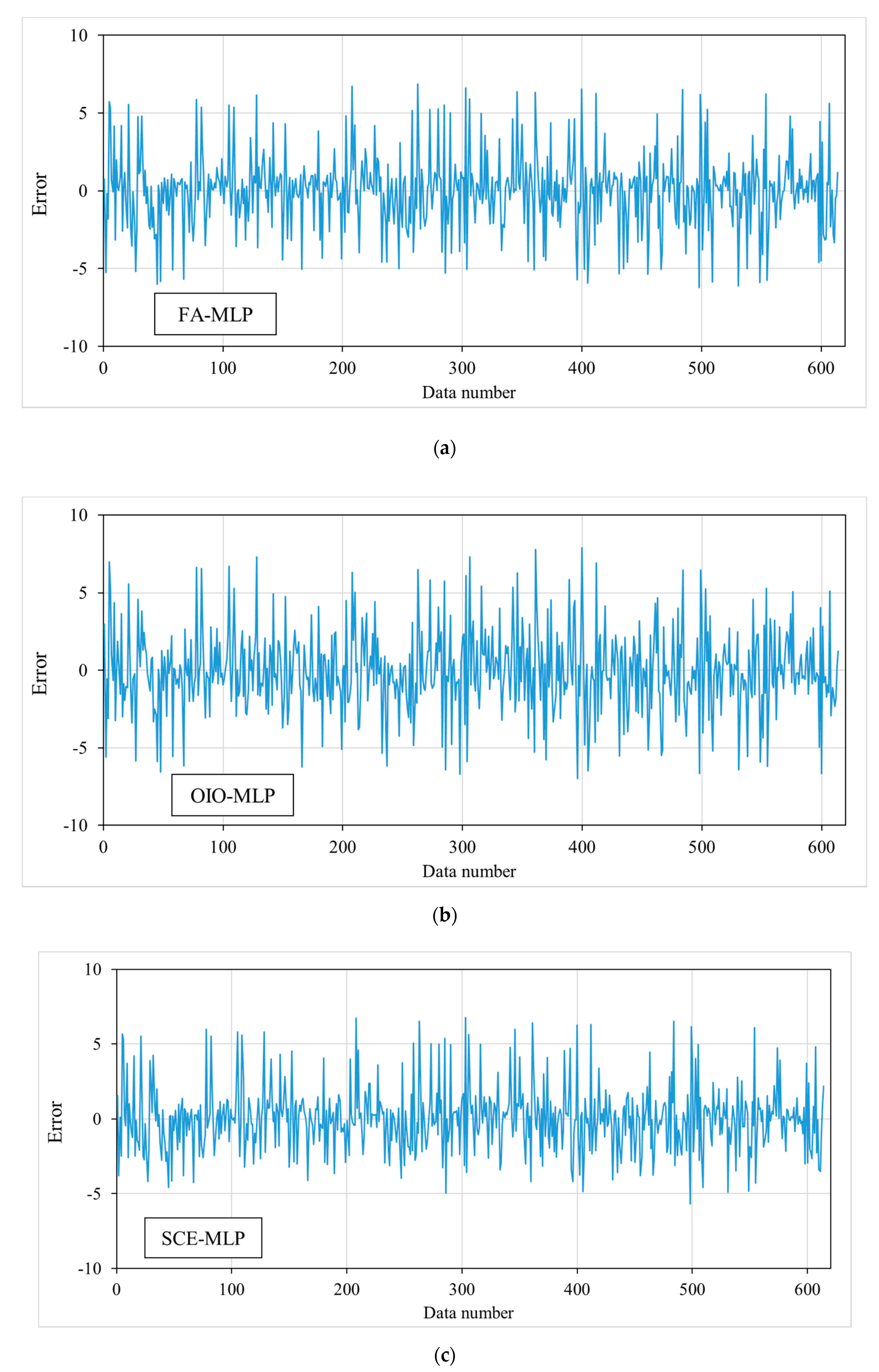
3.2. Incorporated MLP with Optimizers

Once the metaheuristic algorithms are synthesized with the MLP, four ensembles of FA-MLP, OIO-MLP, SCE-MLP, and TLBO-MLP are created. Each ensemble is fed by training samples to infer the dependency between the HL and the corresponding factors. With respect to the optimization behavior of the models, 1000 repetitions are considered for each model to implement the optimization. At each repetition, the RMSE of the results is calculated to report the objective function. Of note is that, since this stage is dedicated to pattern recognition, the RMSE of the training data is reported.

In swarm-based algorithms, the number of the involved population is a key factor. In this study, nine different population sizes (10, 25, 50, 75, 100, 200, 300, 400, and 500) are tested for each model, and the size that gives the lowest RMSE is selected as the optimal complexity. The RMSEs are shown in Figure 3. According to this figure, the lowest RMSE values (2.3838, 2.6256, 2.1448, and 1.9817) are the result of the populations 50, 200, 50, and 300, respectively, for the FA-MLP, OIO-MLP, SCE-MLP, and TLBO-MLP. However, a weaker sensitivity can be seen for the OIO algorithm compared to the other three; the reason for this can be sought in specific characteristics of the optimization strategies. Moreover, Figure 4 depicts the RMSE values obtained for these complexities in all iterations.

Figure 4 also demonstrates that the convergence curve of the TLBO algorithm is slightly lower than the other algorithms. This means that this algorithm has obtained a lower error in adjusting the ANN parameters. Thus, the findings of the algorithm are presented here to create a predictive model. Returning to Figure 2, the output is released from the latest neuron, which deals with seven parameters (six weights and one bias). This neuron itself is fed by six previous layers of neurons, each dealing with nine parameters (eight weights and one bias). Altogether, the network is composed of sixty-one variables that are optimized by metaheuristic approaches. Equation (4) calculates the HL from the TLBO method when it receives six parameters distinguished by K1, K2, K3, K4, K5, and K6, which are the responses of the neurons in the hidden layer:

HL _TLBO-MLP = 0.303606 × K1 − 0.311304 × K2 − 0.276431 × K3 + 0.137188 × K4 + 0.689859 × K5 − 0.265206 × K6 + 0.831238

(4)

These middle terms of the above relationship are functions of the input parameters described in Equations (5)–(10):

K1 = Tansig (−0.756894 × RC + 0.867454 × SA + 0.841520 × WA + 0.216126 × RA + 0.680434 × OH − 0.362683 × OR − 0.323011 × GA − 0.537092 × GAD + 1.751447)

(5)

K2 = Tansig (−0.527296 × RC − 0.057151 × SA − 0.263581 × WA + 0.474892 × RA + 0.420216 × OH + 0.475592 × OR + 0.798177 × GA − 1.204743 × GAD + 1.050868)

(6)

K3 = Tansig (0.645523 × RC − 0.058418 × SA − 0.344279 × WA − 0.897648 × RA − 0.794700 × OH − 0.474246 × OR + 0.875500 × GA + 0.316534 × GAD − 0.350289)

(7)

K4 = Tansig (−0.009316 × RC − 1.121579 × SA − 0.760253 × WA − 0.924062 × RA + 0.169935 × OH + 0.150478 × OR − 0.217070 × GA − 0.528228 × GAD − 0.350289)

(8)

K5 = Tansig (0.029189 × RC + 0.665102 × SA + 0.559293 × WA + 0.741565 × RA − 0.692446 × OH − 0.443736 × OR − 0.864550 × GA − 0.581201 × GAD + 1.050868)

(9)

K6 = Tansig (−0.488121 × RC + 0.222809 × SA + 0.754266 × WA + 1.225463 × RA − 0.156798 × OH + 0.028737 × OR + 0.214770 × GA − 0.798401 × GAD − 1.751447)

(10)

where, for a typical input x,

$$Tansig \left(x\right)=\frac{2}{1+e^{-2x}}-1$$

(11)

3.3. Prediction Results

In this section, the outputs (i.e., the predicted HLs) are compared to the target values (i.e., the measured HLs) to assess the effectiveness of the implemented models. The results of the training phase are presented in Figure 5, which depicts the difference between each set of output and target HLs. In this phase, the obtained error values range in [−6.2053, 6.8793], [−6.9659, 7.8776], [−5.6939, 6.7539], and [−4.1923, 6.5126] for the predictions of the FA-MLP, OIO-MLP, SCE-MLP, and TLBO-MLP, respectively.

The RMSE values, as mentioned in the previous section, are 2.3838, 2.6256, 2.1448, and 1.9817. In addition to this, the calculated MAEs (1.6821, 1.9568, 1.5466, and 1.4626) denote a low level of training error for all four models. Meanwhile, the obtained values of R² indicate a consistency of more than 93% of target and output HLs.

The testing results are also evaluated using the cited accuracy criteria. Needless to say, since the testing data are not first given to the networks; the results of this section reflect the capability of the trained models for predicting the HL for unrealized conditions. The testing results are depicted in Figure 6. Along with the calculated error values, their frequency of is also depicted in the form of histogram charts.

In the testing phase, the RMSEs (2.5456, 2.7099, 2.2774, and 2.1103) indicate that the weights (and biases) tuned by the metaheuristic algorithms can construct capable MLPs. Further, the MAEs of 1.7979, 1.9278, 1.6077, and 1.5804 show a reasonable generalization error for all four ensembles. Moreover, the consistency of the testing results is shown in Figure 7. The calculated R²s (0.9438, 0.9373, 0.9556, and 0.9610) give a high accuracy in predicting the HL.

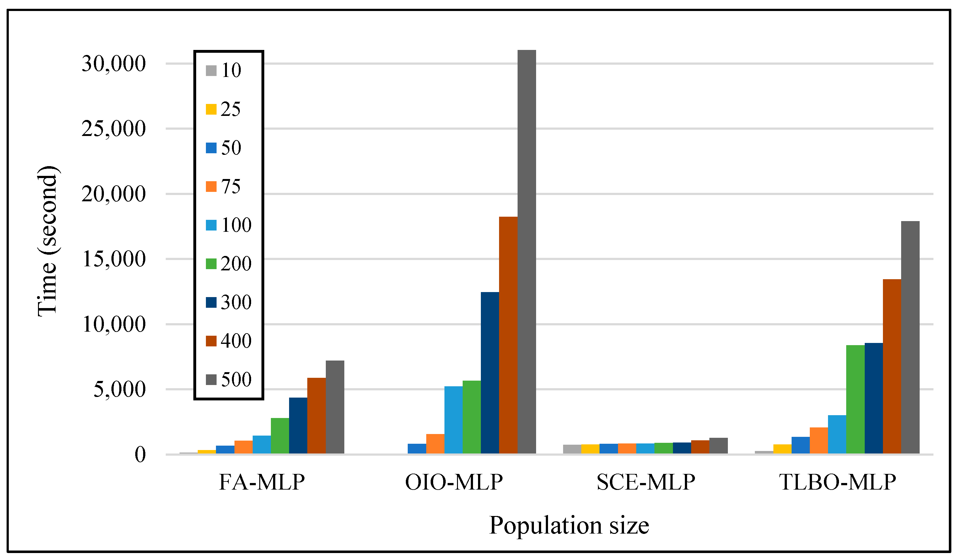
3.4. Efficiency Comparison

Considering the results in both the learning and prediction phases, the models with a lower RMSE (or MAE) and a larger R² are selected as the most accurate predictors of the HL. To this end,

Table 1. Obtained statistical indices in HL modeling of this study compared to [49,51,78,79].

Study	Models	Network Results
		Training			Testing
		RMSE	MAE	R2	RMSE	MAE	R2
This study	FA-MLP	2.3838	1.6821	0.9426	2.5456	1.7979	0.9438
	OIO-MLP	2.6256	1.9568	0.9304	2.7099	1.9278	0.9373
	SCE-MLP	2.1448	1.5466	0.9536	2.2774	1.6077	0.9556
	TLBO-MLP	1.9817	1.4626	0.9604	2.1103	1.5804	0.9610
[49]	ABC-MLP	2.9855	2.1197	0.9120	2.6159	1.9111	0.9349
	PSO-MLP	2.9736	2.1479	0.9126	2.5693	1.8630	0.9370
[78]	GA-MLP	2.9986	2.1797	0.8711	2.8878	2.0622	0.9076
	ICA-MLP	2.8050	2.0068	0.8816	2.7819	2.0089	0.9115
[79]	WDO-MLP	2.5896	1.7944	0.9344	2.8312	1.9863	0.9213
	WOA-MLP	2.6998	1.9702	0.9287	2.9213	2.1921	0.9154
	SHO-MLP	4.2283	3.2232	0.8337	4.1501	3.1092	0.8385
	SSA-MLP	2.4321	1.6737	0.9421	2.7527	1.9178	0.9248
[51]	GOA-MLP	2.3715	1.6934	0.9432	2.4459	1.7373	0.9486
	GWO-MLP	2.2959	1.6475	0.9468	2.2899	1.6514	0.9551

presents all obtained accuracy criteria. As shown, without any discrepancy, the MLP made by the weights and biases from the TLBO presents the most reliable understanding of the HL and also the most accurate prediction of this parameter. Subsequently, the SCE emerges as the second promising optimizer, followed by the FA and OIO.

Table 1 also provides the results of three previous works [49,51,78,79]. In these studies, six different hybrids of the MLP network (based on ABC [80], PSO [81], the genetic algorithm [82], the imperialist competitive algorithm (ICA) [83], wind-driven optimization (WDO) [84], the whale optimization algorithm (WOA) [85], spotted hyena optimization (SHO) [86], the salp swarm algorithm (SSA) [87], GOA [88], and GWO [89]) were employed to predict the HL using the same dataset. At a glance, the TLBO and SCE algorithms used in this study outperform the listed models in both the training and testing phases. This indicates that our work has achieved the defined objective of introducing more capable HL evaluative tools.

Furthermore, Figure 8 shows the computation time taken by each algorithm to optimize the MLP. According to this chart, there is not a significant difference between the performance of the models for populations smaller than 75. Implementing the best fitted populations of the FA-MLP, OIO-MLP, SCE-MLP, and TLBO-MLP (i.e., 50, 200, 50, and 300, respectively) takes around 654, 5652, 794, and 8547 s. The optimum TLBO-MLP, despite having the best accuracy for predicting the HL, is the most time-consuming approach. At the same time, the column of the SCE experiences the smallest change and reaches at most 1261 s.

3.5. Discussion

Overall, the superiority of intelligent models over traditional and experimental approaches is widely accepted in many engineering measurements. Apart from a satisfying accuracy provided by these models, the ease of implementation is a determining advantage for their use. In the case of energy-efficiency analysis, for example, there might be some drawbacks associated with using forward modeling approaches (low capability for occupied buildings [90]) and popular simulation packages (different accuracy of simulation [91]). Therefore, indirect evaluative models, and more particularly the models offered in this paper, are preferable over costly and destructive techniques. This is further stressed when an optimal methodology is developed utilizing metaheuristic techniques. In other words, the use of optimization algorithms creates capable ensembles that operate at optimum conditions.

From an applicability point of view, practical usages can be defined for the suggested methodologies. Two examples are:

(a)

With an upcoming construction project, the suggested models can give an accurate early measurement of the required thermal load with respect to the dimensions and building characteristics. The models would effectively assist engineers and owners in providing suitable HVAC systems.

(b)

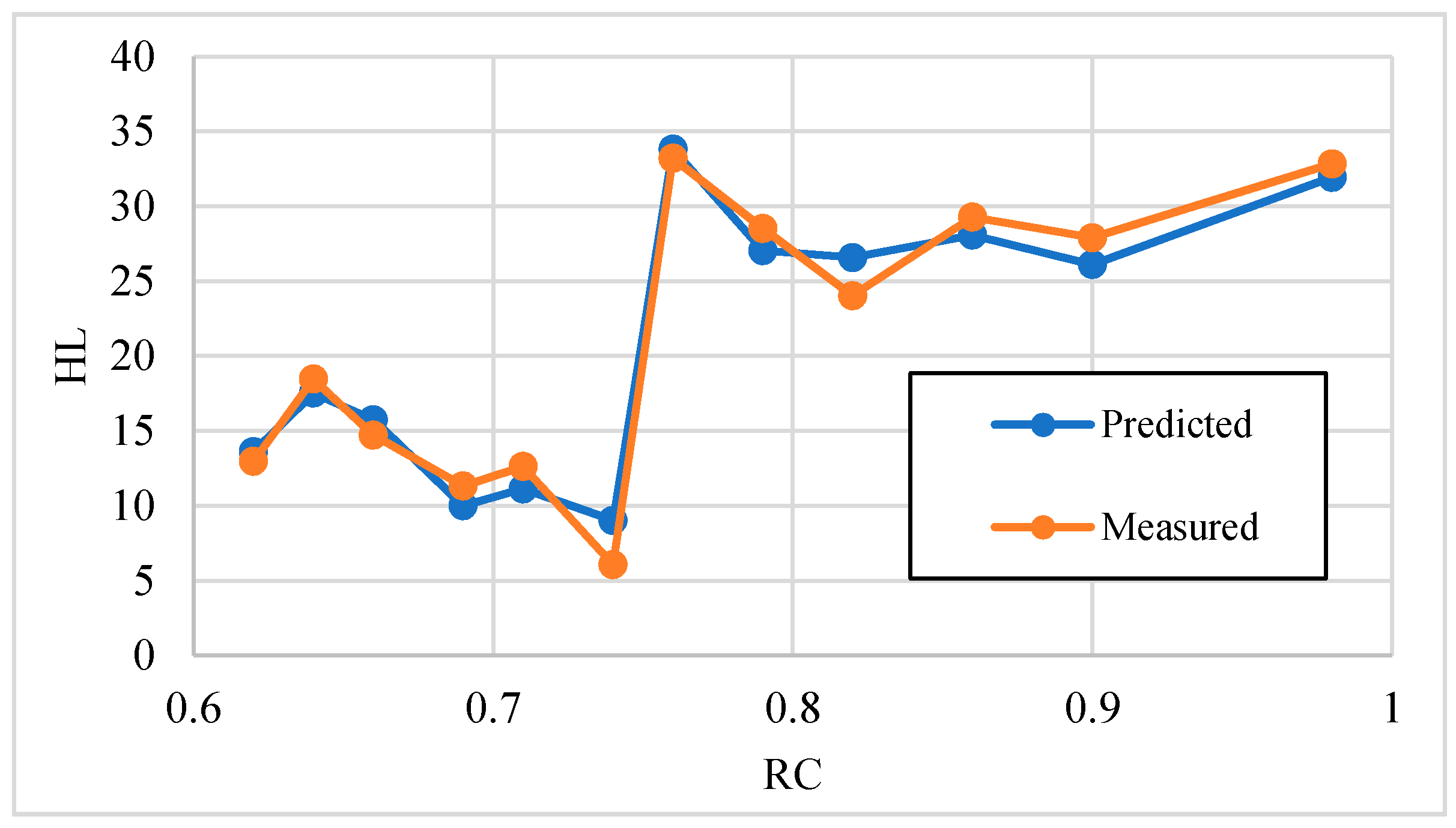
Another form of early-stage assistance would be the proper design of the building itself and tuning the architecture through input parameters (i.e., RA, RC, GA, WA, OH, SA, OR, and GAD) in reconstruction projects. In this sense, it is also possible to investigate the effect of each input parameter separately to achieve an understanding of the thermal load behavior. Figure 9 shows the behavior of the HL with an increase in RC. As shown, the trend is not regular and easy to predict; however, it is nicely predicted by the TLBO-MLP. Hence, this algorithm can give reliable approximations for real-world buildings, too.

In this regard, it is also worth noting that the suggested model was presented in the form of an explicit mathematical formula that is more convenient to use compared to the GUI form in MATLAB.

Despite various benefits that come after solving an optimization problem, taking the appropriate time to find a global solution is required. Hence, having a balance between the time effectiveness and accuracy of the models can influence choosing the most efficient model. However, the authors believe that properly setting the hyper-parameters of the optimizers, as well as performing feature validity analysis, can result in a less complicated problem space, and, consequently, more efficient solutions. Although the TLBO was the most accurate model, the SCE-based models were considerably more time-effective. This necessitates selecting the appropriate methodology with respect to both time and accuracy. For example, in projects for which time is not an issue, using the most accurate mode (i.e., no matter how time-consuming) is logical, whereas in time-sensitive applications, a tolerance may be considered for the accuracy to reach a faster solution. However, it should be noted that, overall, the performance of the models was not that different, and all models would properly serve practical usages.

The dataset used creates a relatively large network and extended problem space due to the number of records and input parameters. In such situations, it is recommended to perform feature selection to use only the most contributive parameters. For instance, according to the importance assessment carried out by Wu et al. [92] on the same data, the role of GA and RC is considerably more involved than other parameters, whereas OR and OH have the smallest influence on the HL. This point should result in a more efficient simulation for future research.

4. Conclusions

This paper presented a comparison between four novel metaheuristic techniques, namely FA, OIO, SCE, and TLBO, for analyzing and predicting the heating load of residential buildings. These algorithms played the role of optimizer for an artificial neural network. The models estimated the HL for 768 thermal load conditions. The outcomes are as follows:

• According to the sensitivity analysis carried out, the best complexities of the FA-MLP, OIO-MLP, SCE-MLP, and TLBO-MLP ensembles result for the swarm sizes of 50, 200, 50, and 300, respectively.
• Compared to other algorithms, the optimum configuration of the TLBO needed considerably higher computation time for optimizing the MLP.
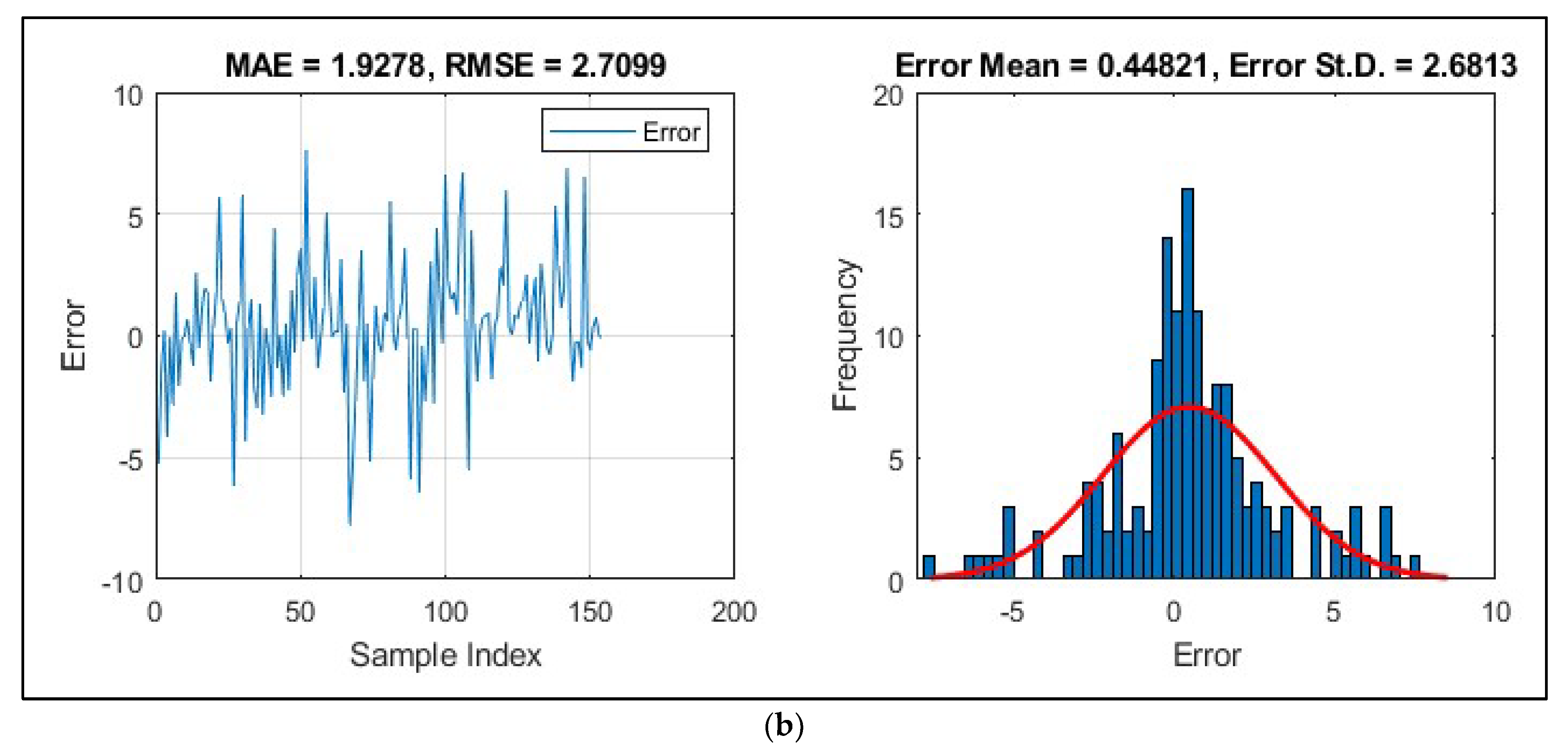
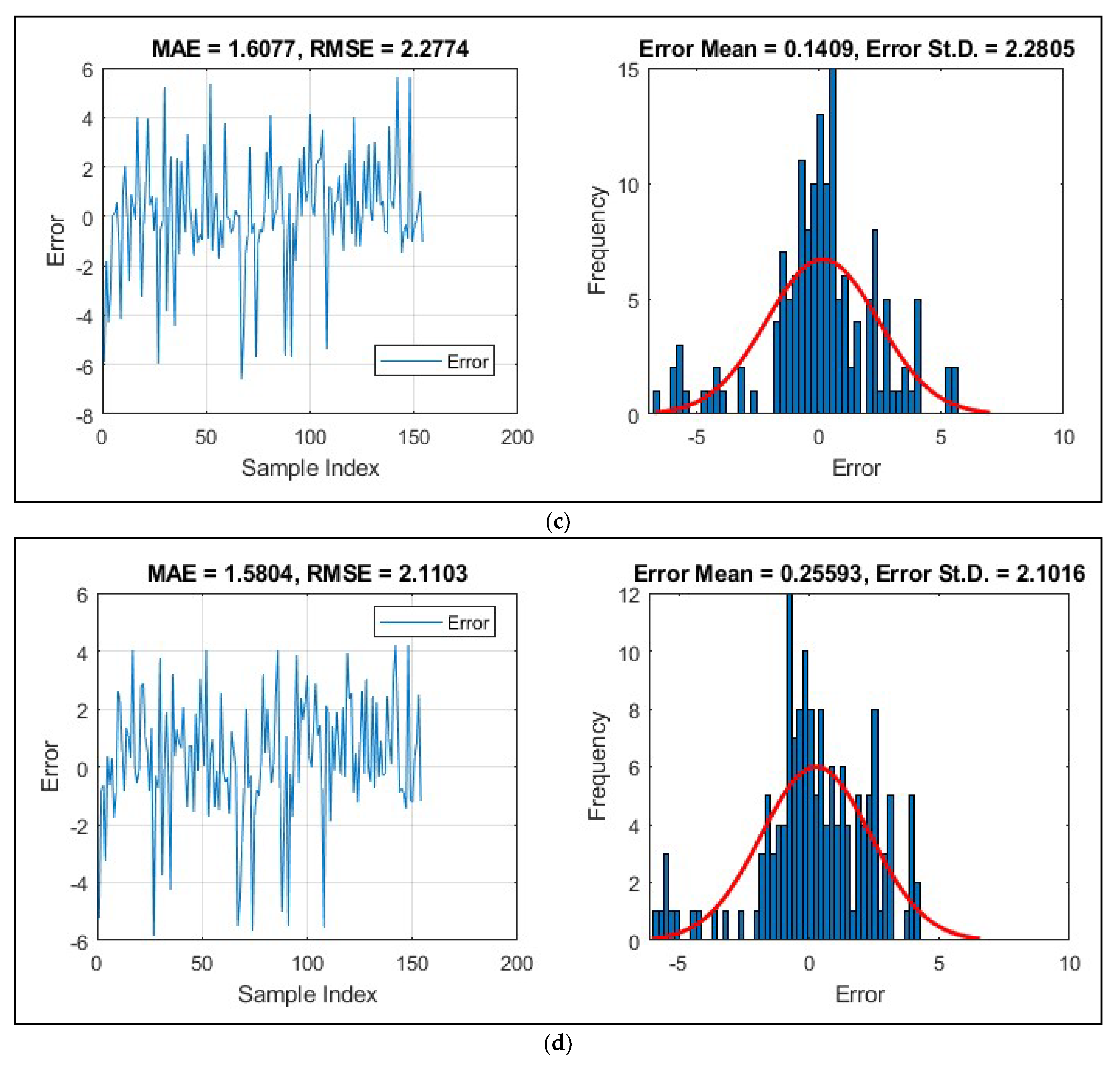
• Considering the accuracy evaluation (the MEAs of 1.6821, 1.9568, 1.5466, and 1.4626), all four ensembles attained a good perception of the relationship between the HL and influential parameters.
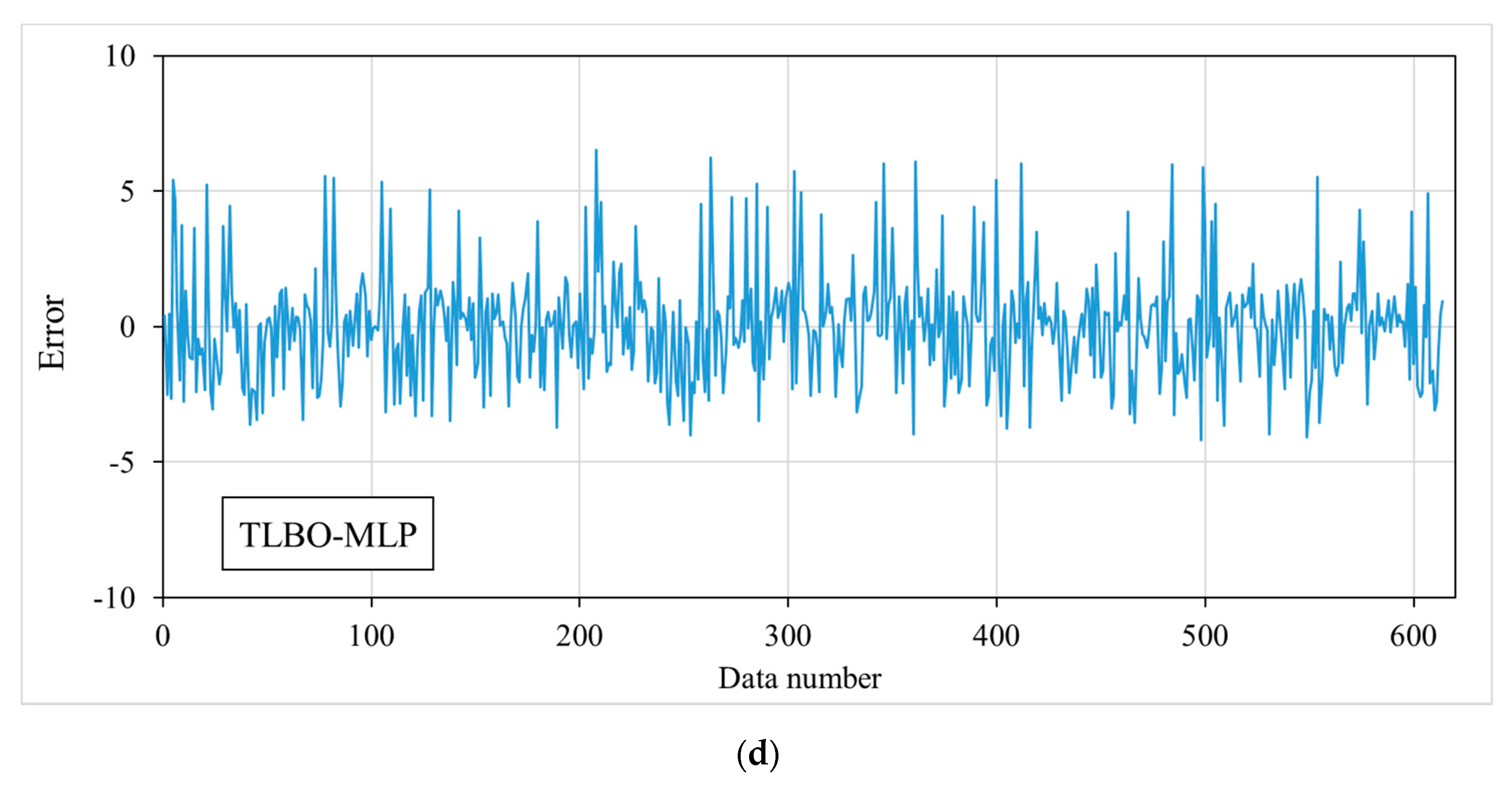
• In the testing phase, the calculated error values of 1.7979, 1.9278, 1.6077, and 1.5804 indicated a low prediction error and the success of the implemented models.
• By comparison, the TLBO-MLP came up to be the strongest model, followed by SCE-MLP, FA-MLP, and OIO-MLP.
• The TLBO and SCE surpassed several other optimizers, including those used in the literature.

The TLBO-MLP was introduced as a practically applicable methodology, but potential ideas were also presented for future projects with respect to the limitations of the study, such as data improvement and future selection, optimizing the characteristics of a building using the model, comparison with more time-efficient tools, etc.

References

- McQuiston, F.C.; Parker, J.D. Heating, Ventilating, and Air Conditioning: Analysis and Design; John Wiley & Sons: Hoboken, NJ, USA, 1982. [Google Scholar]
- Ihara, T.; Gustavsen, A.; Jelle, B.P. Effect of facade components on energy efficiency in office buildings. Appl. Energy 2015, 158, 422–432. [Google Scholar] [CrossRef]
- Rosen, S.L. Using BIM in HVAC design. Ashrae J. 2010, 52, 24. [Google Scholar]
- Ikeda, S.; Ooka, R. Metaheuristic optimization methods for a comprehensive operating schedule of battery, thermal energy storage, and heat source in a building energy system. Appl. Energy 2015, 151, 192–205. [Google Scholar] [CrossRef]
- Sonmez, Y.; Guvenc, U.; Kahraman, H.T.; Yilmaz, C. A Comperative Study on Novel Machine Learning Algorithms for Estimation of Energy Performance of Residential Buildings. In Proceedings of the 2015 3rd International Istanbul Smart Grid Congress and Fair (ICSG), Istanbul, Turkey, 29–30 April 2015; pp. 1–7. [Google Scholar]
- Lu, N.; Wang, H.; Wang, K.; Liu, Y. Maximum probabilistic and dynamic traffic load effects on short-to-medium span bridges. Comput. Model. Eng. Sci. 2021, 127, 345–360. [Google Scholar] [CrossRef]
- Chen, Y.; Lin, H.; Cao, R.; Zhang, C. Slope stability analysis considering different contributions of shear strength parameters. Int. J. Geomech. 2021, 21, 04020265. [Google Scholar] [CrossRef]
- Zhang, S.-W.; Shang, L.-Y.; Zhou, L.; Lv, Z.-B. Hydrate Deposition Model and Flow Assurance Technology in Gas-Dominant Pipeline Transportation Systems: A Review. Energy Fuels 2022, 36, 1747–1775. [Google Scholar] [CrossRef]
- Liu, E.; Li, D.; Li, W.; Liao, Y.; Qiao, W.; Liu, W.; Azimi, M. Erosion simulation and improvement scheme of separator blowdown system—A case study of Changning national shale gas demonstration area. J. Nat. Gas Sci. Eng. 2021, 88, 103856. [Google Scholar] [CrossRef]
- Peng, S.; Zhang, Y.; Zhao, W.; Liu, E. Analysis of the influence of rectifier blockage on the metering performance during shale gas extraction. Energy Fuels 2021, 35, 2134–2143. [Google Scholar] [CrossRef]
- Zhang, W.; Tang, Z. Numerical modeling of response of CFRP–Concrete interfaces subjected to fatigue loading. J. Compos. Constr. 2021, 25, 04021043. [Google Scholar] [CrossRef]
- Peng, S.; Chen, Q.; Liu, E. The role of computational fluid dynamics tools on investigation of pathogen transmission: Prevention and control. Sci. Total Environ. 2020, 746, 142090. [Google Scholar] [CrossRef]
- Wei, J.; Xie, Z.; Zhang, W.; Luo, X.; Yang, Y.; Chen, B. Experimental study on circular steel tube-confined reinforced UHPC columns under axial loading. Eng. Struct. 2021, 230, 111599. [Google Scholar] [CrossRef]
- Mou, B.; Bai, Y. Experimental investigation on shear behavior of steel beam-to-CFST column connections with irregular panel zone. Eng. Struct. 2018, 168, 487–504. [Google Scholar] [CrossRef]
- Xie, S.-J.; Lin, H.; Chen, Y.-F.; Wang, Y.-X. A new nonlinear empirical strength criterion for rocks under conventional triaxial compression. J. Cent. South Univ. 2021, 28, 1448–1458. [Google Scholar] [CrossRef]
- Ju, B.-K.; Yoo, S.-H.; Baek, C. Economies of Scale in City Gas Sector in Seoul, South Korea: Evidence from an Empirical Investigation. Sustainability 2022, 14, 5371. [Google Scholar] [CrossRef]
- Liu, Z.; Fang, L.; Jiang, D.; Qu, R. A machine-learning based fault diagnosis method with adaptive secondary sampling for multiphase drive systems. IEEE Trans. Power Electron. 2022, 37, 8767–8772. [Google Scholar] [CrossRef]
- Yahya, S.I.; Aghel, B. Estimation of kinematic viscosity of biodiesel-diesel blends: Comparison among accuracy of intelligent and empirical paradigms. Renew. Energy 2021, 177, 318–326. [Google Scholar] [CrossRef]
- Moayedi, H.; Mehrabi, M.; Kalantar, B.; Abdullahi Mu’azu, M.; Rashid, A.S.A.; Foong, L.K.; Nguyen, H. Novel hybrids of adaptive neuro-fuzzy inference system (ANFIS) with several metaheuristic algorithms for spatial susceptibility assessment of seismic-induced landslide. Geomat. Nat. Hazards Risk 2019, 10, 1879–1911. [Google Scholar] [CrossRef] [Green Version]
- Braspenning, P.J.; Thuijsman, F.; Weijters, A.J.M.M. Artificial Neural Networks: An Introduction to ANN Theory and Practice; Springer Science & Business Media: Berlin/Heidelberg, Germany, 1995; Volume 931. [Google Scholar]
- Yahya, S.I.; Rezaei, A.; Aghel, B. Forecasting of water thermal conductivity enhancement by adding nano-sized alumina particles. J. Therm. Anal. Calorim. 2021, 145, 1791–1800. [Google Scholar] [CrossRef]
- Peng, S.; Chen, R.; Yu, B.; Xiang, M.; Lin, X.; Liu, E. Daily natural gas load forecasting based on the combination of long short term memory, local mean decomposition, and wavelet threshold denoising algorithm. J. Nat. Gas Sci. Eng. 2021, 95, 104175. [Google Scholar] [CrossRef]
- Seyedashraf, O.; Mehrabi, M.; Akhtari, A.A. Novel approach for dam break flow modeling using computational intelligence. J. Hydrol. 2018, 559, 1028–1038. [Google Scholar] [CrossRef]
- Pinkus, A. Approximation theory of the MLP model in neural networks. Acta Numer. 1999, 8, 143–195. [Google Scholar] [CrossRef]
- Gao, W.; Alsarraf, J.; Moayedi, H.; Shahsavar, A.; Nguyen, H. Comprehensive preference learning and feature validity for designing energy-efficient residential buildings using machine learning paradigms. Appl. Soft Comput. 2019, 84, 105748. [Google Scholar] [CrossRef]
- Ahmad, A.; Ghritlahre, H.K.; Chandrakar, P. Implementation of ANN technique for performance prediction of solar thermal systems: A Comprehensive Review. Trends Renew. Energy 2020, 6, 12–36. [Google Scholar] [CrossRef] [Green Version]
- Liu, T.; Tan, Z.; Xu, C.; Chen, H.; Li, Z. Study on deep reinforcement learning techniques for building energy consumption forecasting. Energy Build. 2020, 208, 109675. [Google Scholar] [CrossRef]
- Hornik, K. Approximation capabilities of multilayer feedforward networks. Neural Netw. 1991, 4, 251–257. [Google Scholar] [CrossRef]
- Ren, Z.; Motlagh, O.; Chen, D. A correlation-based model for building ground-coupled heat loss calculation using Artificial Neural Network techniques. J. Build. Perform. Simul. 2020, 13, 48–58. [Google Scholar] [CrossRef]
- Mohammadhassani, M.; Nezamabadi-Pour, H.; Suhatril, M.; Shariati, M. Identification of a suitable ANN architecture in predicting strain in tie section of concrete deep beams. Struct. Eng. Mech. 2013, 46, 853–868. [Google Scholar] [CrossRef]
- Sadeghi, A.; Younes Sinaki, R.; Young, W.A.; Weckman, G.R. An Intelligent Model to Predict Energy Performances of Residential Buildings Based on Deep Neural Networks. Energies 2020, 13, 571. [Google Scholar] [CrossRef] [Green Version]
- Sholahudin, S.; Han, H. Simplified dynamic neural network model to predict heating load of a building using Taguchi method. Energy 2016, 115, 1672–1678. [Google Scholar] [CrossRef]
- Khalil, A.J.; Barhoom, A.M.; Abu-Nasser, B.S.; Musleh, M.M.; Abu-Naser, S.S. Energy Efficiency Predicting using Artificial Neural Network. Int. J. Acad. Pedagog. Res. 2019, 3, 1–7. [Google Scholar]
- Ryu, J.-A.; Chang, S. Data Driven Heating Energy Load Forecast Modeling Enhanced by Nonlinear Autoregressive Exogenous Neural Networks. Int. J. Struct. Civ. Eng. Res. 2019. [Google Scholar] [CrossRef]
- Zhao, D.; Ruan, H.; Zhang, Z. Application of artificial intelligence algorithms in the prediction of heating load. In AIP Conference Proceedings; AIP Publishing LLC: Melville, NY, USA, 2019; p. 020040. [Google Scholar]
- Adedeji, P.A.; Akinlabi, S.; Madushele, N.; Olatunji, O.O. Hybrid adaptive neuro-fuzzy inference system (ANFIS) for a multi-campus university energy consumption forecast. Int. J. Ambient Energy 2022, 43, 1685–1694. [Google Scholar] [CrossRef]
- Ahmad, T.; Chen, H. Nonlinear autoregressive and random forest approaches to forecasting electricity load for utility energy management systems. Sustain. Cities Soc. 2019, 45, 460–473. [Google Scholar] [CrossRef]
- Namlı, E.; Erdal, H.; Erdal, H.I. Artificial Intelligence-Based Prediction Models for Energy Performance of Residential Buildings. In Recycling and Reuse Approaches for Better Sustainability; Springer: Berlin/Heidelberg, Germany, 2019; pp. 141–149. [Google Scholar]
- Yepes, V.; Martí, J.V.; García, J. Black hole algorithm for sustainable design of counterfort retaining walls. Sustainability 2020, 12, 2767. [Google Scholar] [CrossRef] [Green Version]
- Jamal, A.; Tauhidur Rahman, M.; Al-Ahmadi, H.M.; Ullah, I.; Zahid, M. Intelligent intersection control for delay optimization: Using meta-heuristic search algorithms. Sustainability 2020, 12, 1896. [Google Scholar] [CrossRef] [Green Version]
- Jitkongchuen, D.; Pacharawongsakda, E. Prediction Heating and Cooling Loads of Building Using Evolutionary Grey Wolf Algorithms. In Proceedings of the 2019 Joint International Conference on Digital Arts, Media and Technology with ECTI Northern Section Conference on Electrical, Electronics, Computer and Telecommunications Engineering (ECTI DAMT-NCON), Nan, Thailand, 30 January–2 February 2019; pp. 93–97. [Google Scholar]
- Ghahramani, A.; Karvigh, S.A.; Becerik-Gerber, B. HVAC system energy optimization using an adaptive hybrid metaheuristic. Energy Build. 2017, 152, 149–161. [Google Scholar] [CrossRef] [Green Version]
- Katebi, J.; Shoaei-parchin, M.; Shariati, M.; Trung, N.T.; Khorami, M. Developed comparative analysis of metaheuristic optimization algorithms for optimal active control of structures. Eng. Comput. 2020, 36, 1539–1558. [Google Scholar] [CrossRef]
- Martin, G.L.; Monfet, D.; Nouanegue, H.F.; Lavigne, K.; Sansregret, S. Energy calibration of HVAC sub-system model using sensitivity analysis and meta-heuristic optimization. Energy Build. 2019, 202, 109382. [Google Scholar] [CrossRef]
- Bamdad Masouleh, K. Building Energy Optimisation Using Machine Learning and Metaheuristic Algorithms. Ph.D. Thesis, Queensland University of Technology, Brisbane, Australia, 2018. [Google Scholar]
- Moayedi, H.; Mu’azu, M.A.; Foong, L.K. Novel Swarm-based Approach for Predicting the Cooling Load of Residential Buildings Based on Social Behavior of Elephant Herds. Energy Build. 2020, 206, 109579. [Google Scholar] [CrossRef]
- Moayedi, H.; Mosavi, A. Electrical Power Prediction through a Combination of Multilayer Perceptron with Water Cycle Ant Lion and Satin Bowerbird Searching Optimizers. Sustainability 2021, 13, 2336. [Google Scholar] [CrossRef]
- Yang, F.; Moayedi, H.; Mosavi, A. Predicting the Degree of Dissolved Oxygen Using Three Types of Multi-Layer Perceptron-Based Artificial Neural Networks. Sustainability 2021, 13, 9898. [Google Scholar] [CrossRef]
- Zhou, G.; Moayedi, H.; Bahiraei, M.; Lyu, Z. Employing artificial bee colony and particle swarm techniques for optimizing a neural network in prediction of heating and cooling loads of residential buildings. J. Clean. Prod. 2020, 254, 120082. [Google Scholar] [CrossRef]
- Bui, D.-K.; Nguyen, T.N.; Ngo, T.D.; Nguyen-Xuan, H. An artificial neural network (ANN) expert system enhanced with the electromagnetism-based firefly algorithm (EFA) for predicting the energy consumption in buildings. Energy 2020, 190, 116370. [Google Scholar] [CrossRef]
- Moayedi, H.; Nguyen, H.; Foong, L. Nonlinear evolutionary swarm intelligence of grasshopper optimization algorithm and gray wolf optimization for weight adjustment of neural network. Eng. Comput. 2021, 37, 1265–1275. [Google Scholar] [CrossRef]
- Moayedi, H.; Mehrabi, M.; Mosallanezhad, M.; Rashid, A.S.A.; Pradhan, B. Modification of landslide susceptibility mapping using optimized PSO-ANN technique. Eng. Comput. 2019, 35, 967–984. [Google Scholar] [CrossRef]
- Moayedi, H.; Mehrabi, M.; Bui, D.T.; Pradhan, B.; Foong, L.K. Fuzzy-metaheuristic ensembles for spatial assessment of forest fire susceptibility. J. Environ. Manag. 2020, 260, 109867. [Google Scholar] [CrossRef]
- Mehrabi, M.; Moayedi, H. Landslide susceptibility mapping using artificial neural network tuned by metaheuristic algorithms. Environ. Earth Sci. 2021, 80, 804. [Google Scholar] [CrossRef]
- Mehrabi, M.; Pradhan, B.; Moayedi, H.; Alamri, A. Optimizing an adaptive neuro-fuzzy inference system for spatial prediction of landslide susceptibility using four state-of-the-art metaheuristic techniques. Sensors 2020, 20, 1723. [Google Scholar] [CrossRef] [Green Version]
- Zhou, G.; Moayedi, H.; Foong, L.K. Teaching–learning-based metaheuristic scheme for modifying neural computing in appraising energy performance of building. Eng. Comput. 2021, 37, 3037–3048. [Google Scholar] [CrossRef]
- Tsanas, A.; Xifara, A. Accurate quantitative estimation of energy performance of residential buildings using statistical machine learning tools. Energy Build. 2012, 49, 560–567. [Google Scholar] [CrossRef]
- Moré, J.J. The Levenberg-Marquardt algorithm: Implementation and theory. In Numerical Analysis; Springer: Berlin/Heidelberg, Germany, 1978; pp. 105–116. [Google Scholar]
- Hecht-Nielsen, R. Theory of the backpropagation neural network. In Neural Networks for Perception; Elsevier: Amsterdam, The Netherlands, 1992; pp. 65–93. [Google Scholar]
- Yang, X.-S. Firefly algorithm. Nat. Inspired Metaheuristic Algorithms 2008, 20, 79–90. [Google Scholar]
- Yang, X.-S. Firefly algorithm, stochastic test functions and design optimisation. arXiv 2010, arXiv:1003.1409. [Google Scholar] [CrossRef]
- Yang, X.-S. Multiobjective firefly algorithm for continuous optimization. Eng. Comput. 2013, 29, 175–184. [Google Scholar] [CrossRef] [Green Version]
- Zeng, Y.; Zhang, Z.; Kusiak, A. Predictive modeling and optimization of a multi-zone HVAC system with data mining and firefly algorithms. Energy 2015, 86, 393–402. [Google Scholar] [CrossRef]
- Kashan, A.H. A new metaheuristic for optimization: Optics inspired optimization (OIO). Comput. Oper. Res. 2015, 55, 99–125. [Google Scholar] [CrossRef]
- Kashan, A.H. An effective algorithm for constrained optimization based on optics inspired optimization (OIO). Comput. Aided Des. 2015, 63, 52–71. [Google Scholar] [CrossRef]
- Jalili, S.; Husseinzadeh Kashan, A. Optimum discrete design of steel tower structures using optics inspired optimization method. Struct. Des. Tall Spec. Build. 2018, 27, e1466. [Google Scholar] [CrossRef]
- Özdemir, M.T.; Öztürk, D. Optimal PID Tuning for Load Frequency Control using Optics Inspired Optimization Algorithm. IJNES 2016, 10, 1–6. [Google Scholar]
- Duan, Q.; Gupta, V.K.; Sorooshian, S. Shuffled complex evolution approach for effective and efficient global minimization. J. Optim. Theory Appl. 1993, 76, 501–521. [Google Scholar] [CrossRef]
- Ira, J.; Hasalová, L.; Jahoda, M. The use of optimization in fire development modeling, The use of optimization techniques for estimation of pyrolysis model input parameters. In Proceedings of the International Conference, Prague, Czechia, 19–20 April 2013. [Google Scholar]
- Meshkat Razavi, H.; Shariatmadar, H. Optimum parameters for tuned mass damper using Shuffled Complex Evolution (SCE) Algorithm. Civ. Eng. Infrastruct. J. 2015, 48, 83–100. [Google Scholar]
- Stewart, I.; Aye, L.; Peterson, T. Global optimisation of chiller sequencing and load balancing using Shuffled Complex Evolution. In Proceedings of the AIRAH and IBPSA’s Australasian Building Simulation 2017 Conference, Melbourne, Australia, 15–16 November 2017. [Google Scholar]
- Yang, T.; Asanjan, A.A.; Faridzad, M.; Hayatbini, N.; Gao, X.; Sorooshian, S. An enhanced artificial neural network with a shuffled complex evolutionary global optimization with principal component analysis. Inf. Sci. 2017, 418–419, 302–316. [Google Scholar] [CrossRef] [Green Version]
- Rao, R.V.; Savsani, V.J.; Vakharia, D. Teaching–learning-based optimization: A novel method for constrained mechanical design optimization problems. Comput. Aided Des. 2011, 43, 303–315. [Google Scholar] [CrossRef]
- Talatahari, S.; Taghizadieh, N.; Goodarzimehr, V. Hybrid Teaching-Learning-Based Optimization and Harmony Search for Optimum Design of Space Trusses. J. Optim. Ind. Eng. 2020, 13, 177–194. [Google Scholar]
- Shukla, A.K.; Singh, P.; Vardhan, M. An adaptive inertia weight teaching-learning-based optimization algorithm and its applications. Appl. Math. Model. 2020, 77, 309–326. [Google Scholar] [CrossRef]
- Nguyen, H.; Mehrabi, M.; Kalantar, B.; Moayedi, H.; Abdullahi, M.A.M. Potential of hybrid evolutionary approaches for assessment of geo-hazard landslide susceptibility mapping. Geomat. Nat. Hazards Risk 2019, 10, 1667–1693. [Google Scholar] [CrossRef]
- Mehrabi, M. Landslide susceptibility zonation using statistical and machine learning approaches in Northern Lecco, Italy. Nat. Hazards 2022, 111, 901–937. [Google Scholar] [CrossRef]
- Tien Bui, D.; Moayedi, H.; Anastasios, D.; Kok Foong, L. Predicting heating and cooling loads in energy-efficient buildings using two hybrid intelligent models. Appl. Sci. 2019, 9, 3543. [Google Scholar] [CrossRef] [Green Version]
- Guo, Z.; Moayedi, H.; Foong, L.K.; Bahiraei, M. Optimal modification of heating, ventilation, and air conditioning system performances in residential buildings using the integration of metaheuristic optimization and neural computing. Energy Build. 2020, 214, 109866. [Google Scholar] [CrossRef]
- Karaboga, D. An Idea Based on Honey Bee Swarm for Numerical Optimization; Technical Report-tr06; Engineering Faculty, Computer Engineering Department, Erciyes University: Kayseri, Turkey, 2005. [Google Scholar]
- Kennedy, J.; Eberhart, R. Particle Swarm Optimization. In Proceedings of the ICNN’95—International Conference on Neural Networks, Perth, WA, Australia, 27 November–1 December 1995; Volume 4, pp. 1942–1948. [Google Scholar]
- Holland, J.H. Genetic algorithms. Sci. Am. 1992, 267, 66–73. [Google Scholar] [CrossRef]
- Atashpaz-Gargari, E.; Lucas, C. Imperialist competitive algorithm: An algorithm for optimization inspired by imperialistic competition. In Proceedings of the 2007 IEEE Congress on Evolutionary Computation, Singapore, 25–28 September 2007; pp. 4661–4667. [Google Scholar]
- Bayraktar, Z.; Komurcu, M.; Werner, D.H. Wind Driven Optimization (WDO): A novel nature-inspired optimization algorithm and its application to electromagnetics. In Proceedings of the 2010 IEEE Antennas and Propagation Society International Symposium, Toronto, ON, Canada, 11–17 July 2010; pp. 1–4. [Google Scholar]
- Mirjalili, S.; Lewis, A. The whale optimization algorithm. Adv. Eng. Softw. 2016, 95, 51–67. [Google Scholar] [CrossRef]
- Dhiman, G.; Kumar, V. Multi-objective spotted hyena optimizer: A Multi-objective optimization algorithm for engineering problems. Knowl. Based Syst. 2018, 150, 175–197. [Google Scholar] [CrossRef]
- Mirjalili, S.; Gandomi, A.H.; Mirjalili, S.Z.; Saremi, S.; Faris, H.; Mirjalili, S.M. Salp Swarm Algorithm: A bio-inspired optimizer for engineering design problems. Adv. Eng. Softw. 2017, 114, 163–191. [Google Scholar] [CrossRef]
- Saremi, S.; Mirjalili, S.; Lewis, A. Grasshopper optimisation algorithm: Theory and application. Adv. Eng. Softw. 2017, 105, 30–47. [Google Scholar] [CrossRef] [Green Version]
- Mirjalili, S.; Mirjalili, S.M.; Lewis, A. Grey wolf optimizer. Adv. Eng. Softw. 2014, 69, 46–61. [Google Scholar] [CrossRef] [Green Version]
- Park, J.; Lee, S.J.; Kim, K.H.; Kwon, K.W.; Jeong, J.-W. Estimating thermal performance and energy saving potential of residential buildings using utility bills. Energy Build. 2016, 110, 23–30. [Google Scholar] [CrossRef]
- Yezioro, A.; Dong, B.; Leite, F. An applied artificial intelligence approach towards assessing building performance simulation tools. Energy Build. 2008, 40, 612–620. [Google Scholar] [CrossRef]
- Wu, D.; Foong, L.K.; Lyu, Z. Two neural-metaheuristic techniques based on vortex search and backtracking search algorithms for predicting the heating load of residential buildings. Eng. Comput. 2020, 38, 347–660. [Google Scholar] [CrossRef]