Article

Food System Sustainability Metrics: Policies, Quantification, and the Role of Complexity Sciences

1
Made2Coach Consulting, Av. da República, 6, 7º Esq, 1050-191 Lisboa, Portugal
2
Instituto de Telecomunicações, Instituto Superior Técnico-Torre Norte-Piso 10, Av. Rovisco Pais, 1, 1049-001 Lisboa, Portugal
3
Iscte-Instituto Universitário de Lisboa, Av. das Forças Armadas, 1649-026 Lisboa, Portugal
*
Authors to whom correspondence should be addressed.
Sustainability 2021, 13(22), 12408; https://doi.org/10.3390/su132212408
Submission received: 31 August 2021 / Revised: 30 October 2021 / Accepted: 5 November 2021 / Published: 10 November 2021
(This article belongs to the Special Issue Sustainable Food Systems and Circular Bioeconomy)

Abstract

:
The rise of global attention toward sustainability and sustainable development (SD) has provided increased incentives for research development and investment in these areas. Food systems are at the center of human needs and global population growth sustainability concerns. These drives and the need to provide quantified support for related investment projects led to the proliferation of sustainability metrics and frameworks. While questions about sustainability definition and measurement still abound, SD policy design and control increasingly need adequate quantified support instruments. This paper aims to address this need, contributing to a more consistent and integrated application of food system sustainability metrics and quantified management of the implemented solutions. After presenting the relationships between sustainability, resilience, and robustness and summarizing food system sustainability quantification developments so far, we expose complexity sciences’ potential contributions toward SD quantified evaluation, addressing prediction, intangibles, and uncertainty issues. Finding a paramount need to make sense and bring existing sustainability metrics in context for operational use, we conclude that the articulated application of multiple and independent modeling approaches at the micro, meso, and macro levels can better help the development of food SD policies and implemented solution quantified management, with due regard to confidence levels of the results obtained.

1. Introduction

The rise of international major concern and global attention toward sustainability and sustainable development (SD) in the recent years, including the United Nations (UN) Agenda 21, in 1992 [1], the establishment of the 17 UN SD Goals, in 2015 [2], and the European Commission Green Deal, in 2019 [3], has provided increased incentives for the development of research and investment in these areas of knowledge. With food at the base of human needs in a world of an increasing global population, food systems are at the heart of integrated governance and management sustainable solutions, as reflected in the 2020 European Commission Farm to Fork Strategy for a fair, healthy, and environmentally friendly food system [4].
Together with the higher focus placed in SD, the UN call for the development and use of SD indicators [1], and the need to provide quantified support for related investment projects and evaluation of their accomplishments, a plethora of indicators have been identified and strategies to select the most relevant set of them developed [5]. In 2003, more than 500 efforts related to the development of SD quantitative indicators were already recorded [6]. Despite all these efforts, some authors underline that “although most indices are imputed to be concise and transparent—they fail to meet scientific requirements” [7] and that “politically desired sustainability indices are inherently inconsistent and therefore useless if not misleading with respect to concrete policy advice even for certain aspects of sustainability that they have been predominantly built for” [7].
Some of the works undertaken also stress an underlying lack of consensus about what constitutes sustainability [8] and that even though the need for a holistic approach when developing methodologies for sustainability assessment has been widely recognized, existing data reveal disciplinary fragmentation of this assessment [9]. Hand in hand with these efforts, multiple and overlapping definitions of sustainability, resilience, and robustness still require clarification, especially considering the importance of their alignment for global change policy [10]. Moreover, and in spite of the importance of objective quantification to promote unambiguous evidence-based policy making, control, and improvement, questions are raised on whether sustainability can be measured [11] and why resilience assessment quantification misses the point [12].
All these challenges are heightened when the system’s complex longer-term dynamics with nonlinear feedbacks, interacting at multiple cross-scales and cross-levels [13] within an uncertain context, and with possible critical tipping points leading to undesirable regime shifts, or even system collapse, need to be considered. Additionally, as social-ecological systems (SESs)—in which social includes the economic, political, technological, and cultural elements [14]—food systems are complex adaptive systems [14] that are not sustainable in the current overall regime [15], operating on a planet with tight-coupled boundaries whose subsystems often react in abrupt ways when threshold levels are reached [16]. Moreover, considering food systems’ and food security’s key impact on livelihood security and social welfare, food system sustainability requires raised and urgent attention.
Food systems are coupled SESs, in which institutions mediate between social and ecological processes and resources [17] while keeping food security at the core of food system sustainability efforts [18]. In face of all these circumstances, adequate instruments to support quantified approaches to the design of food system SD institutional policies and management of their implementation are eventually more needed than ever.
This paper aims to: (1) provide a contribution toward the clarification of the operational relationships between sustainability, resilience, and robustness; (2) share a background picture on the road traveled so far toward the quantification of food system sustainability, highlighting the challenges faced; (3) present the important role that complexity theory and tools can play in the quantified evaluation of SD policy implementation and food system sustainability; (4) elaborate on the applicable tools to address prediction, intangibles, and uncertainty; and (5) illustrate how complexity theory and tools, used in conjunction with other available frameworks through multiple independent modeling approaches, can better help the development of informed SD policies and the quantified congruent management of the corresponding implemented solutions. More specifically and besides addressing the wide-range and essential transdisciplinary matters that are key to food system sustainability quantification, this work’s contributions focus on: (1) providing an integrated and articulated approach to existing quantified measures of resilience and their relationship with sustainability; (2) presenting a developed and more encompassing quantified definition of sustainability; (3) highlighting the important role complexity science theories and tools can play in modeling the middle path addressing multiple scales and levels typically involved in food systems; and (4) illustrating in a very elementary and simple fashion the application of the presented quantified definitions of resilience and sustainability to a case study, addressing the different (micro, meso, and macro) levels in connection with an agent-based model, together with a macro-level mathematical model.

2. Sustainability Definition and Measuring Challenges

2.1. SD and Sustainability Definitions

As reflected in different definitions, sustainability is about maintaining (or even enhancing) something over time [19,20]. As a minimum and at its essence, sustainability requires staying within limits [21,22]. In the case of SESs, (anthropocentric) sustainability aims at not crossing environmental systems’ thresholds, related to the planet’s carrying capacity, while fostering sustained and, desirably, improved, social well-being and economic conditions. The intended development, while respecting global and transgenerational needs and limitations, is reflected in the 1987 Bruntland Report, SD concept: “development that meets the needs of the present without compromising the ability of future generations to meet their own needs” [23]. In this sense, SD encompasses development within sustainable conditions.
The wide array of distinct systems (composed of systems of systems) interacting in an SES, their complex dynamics, multiple and varied stakeholders, coupling, space and time considerations tend to add serious challenges to the required understanding of the SES behavior and the proper setting of sustainable integrated operation limits. From a broader perspective, while acknowledging the tightly coupled nature of different planetary processes’ boundaries and the nonlinear and abrupt reaction of many Earth subsystems around specific key variables, Rockström et al. [16] proposed a set of process-specific safe operating boundaries for humanity. In the same vein of thought, other authors [24,25] expressed concern with a planetary-scale tipping point, associated with reaching critical thresholds whose values are often not known in advance, highlighting the need to improve biological forecasting and detection of early-warning signals. In particular, Folke et al. [14] exemplified the intertwined nature of SESs, regarding them as complex adaptive systems with frequently unpredictable agent interactions, and using a social-ecological resilience approach to study their dynamics.
The design of adequate models that allow us not only to better understand the studied system but also to infer the expected outcomes of a specific policy implementation is an increasingly challenging task as we expand the scope of analysis and range of complex adaptive systems involved. Despite these challenges, the identification and tracking of parameters that allow us to gain an improved indication of where we are, and how we are moving along, is a relevant helping step. In fact, the major worldwide focus on SD efforts, the ample government support to associated initiatives, and the corresponding political drive toward progress-monitoring measures, as well as the UN Agenda 21 wide call to the development and identification of SD indicators, has led to a multitude of indicator lists [7].

2.2. Sustainability Frameworks, Indices, Indicators, and Metrics

Considering the large number of variables involved in a holistic social-ecological approach to a complex reality with multi- and cross-scale and cross-level dynamics [13], it should not be surprising the appeal of simple monitoring information elements that can provide a quick and intuitive overall picture about how SES policies are progressing. While composite indicators—or indices, in the sense of a compounded value of multiple weighted indicators [26]—are subject to debate regarding their reliability, quality, and consistency [8,26,27], with some authors stating that scientific rules for compounding the indices they reviewed are typically not followed [7], their popularity in connection with the defined SD goals is indisputable. Examples include the UN Global SDG Indicators Database [28] or the Eurostat sustainable development indicators tables [29]. The possibility of a quick global and general view of the progress toward the SDGs is also illustrated by the corresponding dashboard developed by the UN [30].
Given the profusion of possible indices, indicators, and metrics, various frameworks and methods have been presented regarding how to formulate, compare, and select them [5,31,32,33,34,35], including a methodological framework that summarizes best practices in their application at local scales [36]. Despite the enormous efforts and developments that have taken place toward sustainable development, with multiple instruments available to allow us to better monitor how we are progressing toward the defined goals, important steps are seen as still missing and affecting other important contributions to sustainability-oriented policy design and control. In particular, the abrupt ways SESs often react when threshold levels are reached [16], with agents also frequently interacting unpredictably [14] in an increasingly anthropocentric hyperlinked world, should make us more aware that past trends may not predict the future. While sustainability addresses the projection of some attribute, or set of attributes, into the future, our indicator tools tend to only show us the present and past. As stated by Parris and Kates, “characterizing and measuring sustainability involves making choices about how to define and quantify what is being developed, what is being sustained, and for how long” [6]. Without a model that provides us with some informed predictive insight about how the quantity, or quantities, that we need to track can be expected to evolve in the future, our assessment of sustainability will tend to be seriously hampered. In line with the illustration provided by Bell and Morse [11] (Figure 1.3), if we only have a representation of the system parameters of interest over time and just look at their trends, we may be at odds to gauge the sustainability related to those parameters.
On a more conceptual level and to properly proceed toward the adequate modeling of our systems, including adequate and consistent metrics and their required quantification, other interrelated and key issues need to be addressed. First, there is the need to have a clear definition of sustainability. Without it, the establishment of policy goals and decision making at any level is hampered [9]. However, besides the fragmentation of perspectives regarding sustainability assessment, in connection with the various disciplines studying it [9], the debate about sustainability tends to focus on sustainable development matters rather than distinguishing first the notion of sustainability and how to assess it. Additionally, we need to answer how to handle the complex dynamics and the multitude of indicators about what we need to sustain and develop. This paper aims to provide contributions to both questions. However, before proceeding, we need to tackle a sustainability-definition-related issue, which concerns the need for a coherent distinction between sustainability, resilience, and robustness.

2.3. Robustness, Resilience, and Sustainability

While related, in different ways, to the notion of stability, the terms robustness, resilience, and sustainability abound in the literature, although not always reflecting the same conceptual understandings. Acknowledging how the overlap of existing definitions and unclear articulation of these concepts reduce their utility, Anderies et al. [10] provided a key contribution to aligning them for global change policy. According to these authors, while resilience “provides a framework to think about how multiple systems […] interact across scales”, sustainability “provides a framework to translate the understanding [developed through robustness-related concepts and tools] of feedback systems into meaningful action through policy discourse” [10]. In this sense, the concept of sustainability appears closely tied to the global SD challenges, as a “superstructure [or an] analytical framework to guide action” [10], more than a quantifiable metric of a system’s dynamical performance, i.e., sustainability as the ability of a system to maintain (or sustain) something over time, as reflected in a success probability over time.
As stated by Holling, in his seminal paper about the resilience and stability of ecological systems, back in 1973 [37], while stability can be defined as the “ability of a system to return to an equilibrium state after a temporary disturbance”, resilience “determines the persistence of relationships within a system and is a measure of the ability of these systems to absorb changes of state variables, driving variables, and parameters, and still persist”. The property of resilience appears as a counter-balancing element to disrupting forces that tend to drive the system out of its required persistence (even if mutable) boundaries. In this context, higher resilience contributes to higher chances of persistence over time, i.e., to higher sustainability. Resilience is a property and the system’s (desirably reduced) probability of extinction, or sustainability, the result [37,38].
Various notions of resilience are, however, described in the literature. Anderies et al. [10] distinguished between specified resilience (in the sense of “resilience of what to what” [39], focusing on the definition of system boundaries [10]) and general resilience (referring to “broader system-level attributes [including] the capacity for learning and adaptation” [10]). Davoudi and Porter [38], clarified the differences between engineering resilience (measured by the “resistance to disturbance and the speed by which the system returns to equilibrium”), ecological resilience (acknowledging the “possibility of systems to flip into alternative stability domains”), and evolutionary resilience, or socio-ecological resilience (advocating that “the very nature of systems may change over time with or without an external disturbance”). In this last sense, directed to the SES nature of food systems, resilience is the “ability of complex socio-ecological systems to change, adapt, and crucially, transform in response to stresses and strains” [38,40]. This broader notion of resilience goes beyond the system’s capability to absorb disturbance and reorganize [41]. It encompasses also adaptability (“the capacity of actors in the system to influence resilience” [41]) and transformability (“the capacity to create a fundamentally new system when ecological, economic, or social structures make the existing system untenable” [41]).
Addressing the distinction between stability and robustness, Jen [42] argued that even though both of them are “concerned with the persistence, or lack thereof, of the specified features under the specified perturbations”, robustness is a broader concept than stability. Robustness is described as appropriate for measuring feature persistence in systems difficult to parametrize, subject to significant changes, or whose “behavior is generated through adaptive dynamics coupled to strong organizational architecture” [42]. As she also summarized, robustness is an approach to feature persistence in systems for which we do not have the stability theory mathematical tools, as we must focus on perturbations different from those already observed [42]. Anderies et al. [43], while providing a framework to analyze the robustness of SESs from an institutional perspective, suggested that “a SES is robust if it prevents the ecological systems upon which it relies from moving into a new domain of attraction that cannot support a human population, or that will induce a transition that causes long-term human suffering”. While robustness is expected to provide system dynamics performance measures and resilience has evolved into an intellectual framework [10], there is clear proximity between the notion of robustness provided [e.g., 42, 43] and some of the presented characterizations of resilience. Like resilience, robustness is expected to encompass change, including a system’s adaptive processes, which in some contexts, are directed to the preservation of its identity [42]. Folke [44] suggested that while engineering resilience is focused on constancy and recovery (in the vicinity of a stable equilibrium), ecological resilience is focused on robustness (around multiple possible equilibria), and social-ecological resilience is focused on adaptive capacity, learning, innovation, and transformation. According to Anderies et al. [10], it is the precision required by robust control and the corresponding need to have a clear grasp on the system’s boundaries that limit its capacity to address learning, adaptation, and transformation (key elements of resilience).
When considering both sustainability and resilience as frameworks [10], the question arises as to how they relate to each other. Derissen et al. [45] addressed this issue in the context of SESs, highlighting that while sustainability is a normative concept (in line with the Bruntland Report concept of SD [23], aiming at intra- and intergenerational justice), resilience is a descriptive concept (including the notion that resilience is not necessarily a good thing). They further illustrated with a model of two natural capital stocks how the full set of four relationship combinations of the resilience of the system being necessary (or not) and sufficient (or not) for sustainability may hold. In face of the quite different conceptual understandings and applications of these terms, Marchese et al. [46] performed a literature review of 37 journal articles proposing management frameworks for the joint implementation of sustainability and resilience. As described by them, these frameworks could be grouped into three different sets describing: (1) resilience as a component of sustainability; (2) sustainability as a component of resilience; and (3) resilience and sustainability as separate objectives, with their corresponding approaches being either uncorrelated or positively, or negatively, correlated [45]. Addressing this same theme of the increasing literature with different uses of these terms, Redman [47] contrasted adaptation versus transformation, and the prioritization of process versus outcome, as differences between resilience theory and sustainability science. He concluded by stating that “we must rigorously pursue adoption of distinct resilience and sustainability approaches, as well as combinations of the two, allowing each approach to contribute in ways that reflect its strengths” [47].
When referring to the profusion of the sustainability and resilience terms in the literature, it is important to note that the application of these terms tends to be more closely used within the whole body of knowledge related to the still new sustainability science (as a foundation for great change [48]), resilience theory, and (the complex) achievement of the defined SDG than to the operational application of these concepts. As mentioned by Carpenter et al. [39], although the use of resilience as a metaphor or theoretical construct can be inspiring, “much more insight could be gained from empirical analyses, which would require an operational, measurable concept of resilience”. Similar benefits can be gained from the application of an operational, measurable concept of sustainability, particularly if also articulated with the concept of resilience, and efforts in that direction are seen as potentially very useful and needed.
Acknowledging the complexity of food systems, operating at multiple levels and scales and embedded in larger SESs, as well as the challenges imposed by the high levels of uncertainty that may be involved, should not deter us from taking the steps that allow us to tackle those challenges. These steps include the development of the required tools to gain a better, quantified, understanding (however limited it may initially be) of the associated dynamics, making use of a clear and consistent set of definitions, including sustainability- and resilience-related operational concepts and metrics, leveraged by robust control, dynamical systems, and complexity science theory.

2.4. Quantifying Sustainability

In this subsection, we take the following steps: (1) distinguish the notions of weak and strong sustainability; (2) present a proposed definition of sustainability that can accommodate both of those notions; (3) address other works concerning the quantification of sustainability, resilience and stability, the relationships between them, and how these are affected by uncertainty; and finally, (4) elaborate on the quantification of resilience and its quantified relationship with sustainability.
Within our first step, we must underline that, to guide decision making under uncertainty, sustainability needs to be an ex ante assessment concept [45]. As Derissen et al. [45] also suggested:
  • Under those ex ante and uncertain conditions, the sustainability criterion can only be met with some probability;
  • Depending on whether this probability is associated with a notion of maintaining an aggregate wealth or welfare or with the maintenance of separate critical stocks and services above some minimum levels, we can speak, respectively, of a weak, or strong, notion of sustainability.
Regarding the indicated second step, to quantify the sustainability S A of a set A of features of interest on an SES at time t k (considering that all those features hold at time t 0 ), we elaborate on the degree of viability definition provided by Baumgärtner and Quaas [49]. While the definition of viability provided by these authors can be subsumed, under uncertainty, to the notion of strong sustainability (Neumayer 2003, cited in [49]), providing a result of True/False to whether a project is sustainable, the degree of viability provides a continuous (probability) measure of sustainability [49].
We developed this notion of a continuous measure of sustainability in two ways. First, we expanded it to accommodate the possibility of measuring more than just the probability of each of the system’s n relevant individual funds G u (u = 1. …, n)—described by l   N different stock variables g u h ( t ) R   ( h = 1 ,   ,   l ) —and of each of the m relevant individual types of services W j (j = 1, …, m)—which may be provided between funds G x and G y as described by w x y j ( t ) R —being kept within a corresponding sustainable threshold (a strong sustainability requirement). The developed definition admits also that a possible desirable function f i   ( i N ) , including funds, services, or both as variables, can also be considered, with a corresponding threshold f ¯ i associated with a specific i condition (either   , > , < ,   o r     ) . This allows for the inclusion of more complex relationships between funds and services, including eventually an aggregate stock (capital, welfare, etc.) associated with the notion of weak sustainability. Second, we also contemplate the possibility that sustainability-related relationships between these relevant funds, services, and thresholds may change (i.e., depend on time t) throughout the period (from t 0 to t k ) of sustainability analysis. This expansion of the definition scope allows for greater system dynamic behavior considerations, including adaptive, innovative, and even transformative aspects.
S A ( t k ) = m i n i {   P r o b   [   f i   ( g u h ( t ) ,   w x y j ( t ) , t )   i   f ¯ i ( t ) ] i   N , ( h , j , u , x , y ) H × J × U × X × Y , t [ t 0 , t k ] }  
where U, X, Y   {1, …, n}, H   {1, …, l}, and J   {1, …, m}.
If specific probability thresholds are assigned to the satisfaction of each f i   i   f ¯ i condition throughout the analyzed period (from t 0 to t k ), we also obtain a sustainability True/False result as with the viable definition provided by Baumgärtner and Quaas [49]. Additionally, even though the sustainability measure is given by the function f i whose probability to satisfy the condition i   f ¯ i is the lowest, a broader sustainability analysis can be performed by comparing the sustainability of all the remaining features (associated with each of the remaining f i functions).
To better assess this sustainability over time, we need to model the applicable feature’s system dynamics with its environment. The system’s current position in the corresponding state space must be identified and the flows and potential disturbances (external and internal) considered, including how the system and its environment respond, learn, and reconfigure in face of those flows and disturbances. Even without considering the multiple possible future scenarios and the challenges related to assessing the likelihood and impacts of potential developments for which risk assessment data are missing, the complexity of determining the sustainability of a system’s feature, or set of features, tends to become an exponentially increasingly daunting (if feasible) task as the complexity of the system and its interactions grows.
For our third step, we need to start by highlighting that several other important works toward a mathematical quantification of resilience and sustainability, as well as toward the quantification of stability in stochastic systems, have already been made available. Highlighting the need for precise starting definitions, to allow a structural development of a mathematical theory of resilience, Krakovská et al. [50] elaborated on several indicators related to engineering and ecological resilience (e.g., reactivity, latitude in width and in volume, distance to threshold). For this purpose, they started by reviewing the existing indicators within the framework of continuous dynamical systems theory and the generalization of the definitions to general attractors, whenever possible. Using an example of a classic one-dimensional population model, they applied the previously specified definitions in terms of local indicators, basin shape indicators, nonlinear transient dynamics, and variation of parameters [50].
Additionally, a key aspect to be considered when measuring the sustainability of a system’s set of features concerns its relationship with the system’s stability and resilience and how these are measured and affected by uncertainties and perturbations over time. To overcome the potentially highly misleading systems’ behavior outcomes provided by the application of linear stability analysis to situations where the systems are subject to continuous stochastic perturbations, Nolting and Abbott [51] showed how the quasi-potential concept from stochastic analysis more adequately quantifies stability in these situations, including the relative stability of alternative stable states. Even though the quasi-potential concept cannot provide complete information in cases where the system undergoes extreme shocks, it operationalizes one aspect of resilience expressed by Holling [37] as “the height of the lowest point of the basin of attraction [as] a measure of how much the forces have to be changed before all trajectories move to extinction of one or more of the state variables” (Holling, cited in [39]) [51]. Illustrating the differences between asymptotic stability, basin width, and quasi-potential stability metrics, the authors also elaborated on how this last metric is useful for better putting in context other stability-related concepts, such as reactivity, resistance, and persistence [51].
Moving toward the fourth step previously mentioned and concerning the quantification of resilience, Anderies et al. [52] used a grazing management case of a fire-driven rangeland system (to which we return in Section 5) to illustrate the measurement of resilience as the displacement the system can support while maintaining a given function. As such, in this case, they represented the system’s resilience, for each grazing pressure, as the distance (in terms of biomass) between the (desirable) system’s high biomass equilibrium line and the biomass line of unstable equilibrium that can lead the system to the (undesired) zero biomass equilibrium, until the bifurcation point is reached (where these two lines meet and beyond which only the zero biomass equilibrium applies). Referring to that most resilience-related studies focus on it as a theoretical construct and that only in a few cases it has been operationally defined and applied, Martin [53] used a lake eutrophication example and a viability approach [54] to define and illustrate a definition of resilience. In line with the definition that resilience is “the capacity of a system to undergo disturbance and maintain its functions and controls”, resilience was measured as the inverse of restoration cost (considering both an ecological and an economical cost) [53]. To this end, a viability kernel (gathering all system states from which, applying the available control measures, exists at least a trajectory allowing the system to remain within the stated objectives until the specified time scale of interest) and a set-value map (that associates a specific state x with all reachable states y from it after an anticipated disturbance D occurs) were determined. The resilience of the system at state x facing a disturbance D was then defined as the minimum value of the resilience of all possible reachable states y to which the system jumped due to D (measured as the inverse of the minimal cost of restoration among all trajectories starting at y) [53].
Leveraging the aforementioned work [53] and using the rangeland system management case presented by Anderies et al. [52], Martin et al. [55] presented the limitations of attractor-based measures of resilience (defined as the inverse of return time or as proportional to the size of the attraction basin size) and provided a viability-based definition of resilience. This viability-based approach accommodates the possibility that the desired property of the system and respective states do not necessarily correspond to attractors. In this sense, they considered the resilience of the desired property (rather than the resilience of the system), defining a capture basin (including the points outside the viability kernel that can go into it, such as an attraction basin in the case of an attractor), a resilience basin (including the kernel and the capture basin), and a resilience value (associated with each point in space, as the inverse of time to get to the viability kernel) [55]. Like the notion of resilience as the inverse of cost of restoration [53], resilience is here presented with a value associated with each point on the system’s state space and not as a global system metric. It is also important to note that while the quasi-potential metric (corresponding to Holling’s definition of resilience [51]) and other stability-related concepts focus on the strength of the disturbances required to drive a system out of its current basin of attraction, the concept of resilience as the inverse of the cost of restoration provides a measure of the strength of effort required to bring back the system to a desired viability kernel (with resilience being assessed as infinite within this kernel). This distinction relates closely with the concepts of precursor resilience—“ability to accommodate change without catastrophic failure, or a capacity to absorb shocks gracefully (Foster, 1993: 36)” (cited in [56])—and recovery resilience—“ability to respond to singular or unique events (Kendra and Watchendorf, 2003: 42), bouncing back to a state of normalcy—presented by Boin and Etten [56].
In the context of quantifying economic sustainability, Goerner et al. [57] provided a relationship between sustainability and resilience: sustainability is depicted as an inverted U function of diversity/connectivity, whose apex (corresponding to a window of vitality/viability) is achieved at an optimal mix between efficiency (pulling toward lower levels of diversity and redundancy) and resilience (pulling in the opposite direction). Within this concept, a system’s sustainability is described as a single metric capturing the balance between brittleness (insufficient resilience) and stagnancy (insufficient efficiency) [57]. Ulanowicz et al. [58] went a step further in the quantification of system sustainability (that they also equated to robustness), using information theory concepts to define a single metric that reflects a similar tradeoff allotment between a system’s effective performance and reserve capacity. Multiplying total system throughput (T..) respectively to aggregate system indeterminacy (H), average mutual constraint (X), and conditional entropy (Ψ)—in which H = X + Ψ—they obtained the measure of system development capacity (C = T.. ∙ H) as the sum of system ascendency (A = T.. ∙ X) and system reserve (ϕ = T.. ∙ Ψ). This development capacity (C = A + ϕ) reflects the notion that a system’s capacity to adapt and overcome disturbances depends both on its ability to maintain its integrity (reflected in A) as well as the required flexibility (reflected in ϕ) [58]. Providing also a definition of fitness for evolution (F = -ka log(a), with a = A/C), they defined robustness, R, of the system (R = T.. ∙ F) [58].
One final note about sustainability quantification deals with the limitations of modeling a system under conditions that are currently uncertain and were never observed before and whose applicable system’s dynamics are unknown to us. While the concepts and metrics of ascendency and system reserve provide us insights about the sustainability of the system based on its current and past observed behavior, they are eventually limited in informing us about the system’s capability to handle disturbances in case other (not previously observed) behavioral or system organizational dynamics take place under those specific conditions. Levine [12] stressed this point when he stated that “it is impossible to say in advance how resilient people are until they are faced with a test”. One SES example of this matter is provided by the study of coral-reef recovery [59] illustrating: (1) how a “sleeping functional group”—such as the batfishes, not previously associated with coral–algae interactions—reveals itself as capable of performing a particular function but only under exceptional circumstances (in this case, only after the system’s phase shift has occurred, driving the coral-reef recovery); and (2) how species of functional groups that prevent phase shifts—in the studied case, parrotfishes or surgeonfishes (herbivores)—contrary to previous expectations, may not be able to reverse phase shifts once they occur.

3. Sustainable Food System Policy Design and Control

3.1. Toward Sustainable Food Systems

A food system can be described as “a chain of activities from production (‘the field’) to consumption (‘the table’), with particular emphasis on processing and marketing and the multiple transformations of food that these entail” [17]. This chain of activities includes interactions and feedback between human, biological, and geophysical environments [15].
The topic of sustainable SESs, and the transition to sustainable food systems that can accommodate the challenges of ensuring healthy, nutritious, and high-quality food for an increasing global population (from the current 7.6 billion to 9.8 billion in 2050 [60]), respecting the environment and the economic needs of the intervening agents, has seen increasing interest by multiple stakeholders, including the scientific community. Even though the 17 UN SDGs of the 2030 Agenda of the UN address individual sustainable development goals (including SDG2—zero hunger), food and agriculture themes are pervasive elements among them [15]. They must, however, be addressed in an integrated fashion, as each of them reflects only specific aspects of an underlying global complex adaptive system. This complexity—global spread, critical nature (for human survival and well-being), and potential impacts at the social-economic and ecological levels, with prominent problems to tackle—makes the study of food system sustainability a daunting, but most needed, endeavor. The UN Food and Agriculture Organization (FAO) strategic framework 2022-2031 [61] highlights that “690 million people suffered from hunger even before COVID-19, millions more are micronutrient deficient, and an alarmingly growing number of people are overweight across all ages, classes and borders”. As stated in FAO’s 2020 report of the state of food security and nutrition in the world [62], “in a world that produces enough food to feed its entire population, more than 1.5 billion people cannot afford a diet that meets the required levels of essential nutrients and over 3 billion people cannot even afford the cheapest healthy diet”. Besides the essential role that food plays in everyone’s life and the stresses agri-food systems place on the environment, it is also important to consider (from an economical perspective) that they directly employ over 1 billion people worldwide and provide livelihoods to another 3.5 billion [61] (i.e., in total, more than half of the human population).
The concern with the environment, and the need to move to sustainable growth, is reflected in the European Commission Green Deal [3]—aiming at, among other aspects, achieving no net emissions of greenhouse gases in 2050 and decoupling economic growth from resource use—which includes as one of its key elements a “fair, healthy and environmentally friendly food system”. This line of action was more recently presented in the European Commission Farm to Fork Strategy [4] as “a new comprehensive approach to how Europeans value food sustainability”. At the center of this strategy are the needs to ensure sustainable food production and food security, stimulate sustainable food services practices, promote sustainable food consumption (while facilitating the shift to healthy diets), reduce food loss, and combat food fraud [4]. Food security—defined by FAO as the situation “that exists when all people, at all times, have physical, social and economic access to sufficient safe and nutritious food that meets their dietary needs and food preferences for an active and healthy life” [63]—is a core goal of food system sustainability. However, although there are different concepts and goals associated with food system sustainability, often with specific narratives and distinct from the one of global environmental change, there is an increased recognition of the need to address them together due to their close interrelations [15]. Going a step further and mentioning the importance of humans to see themselves embedded in a greater whole (the biosphere), not as separate agents from the rest of nature, Folke et al. [14] underlined the need for a biosphere-based sustainability science, reconnecting approaches and development perspectives in an Anthropocene in which humanity must understand and act responsibly in view of its prominent and heightened power to affect the biosphere.
Defining a sustainable food system as “one that achieves and maintains food security under uncertain and dynamic social-ecological conditions”, Eakin et al. [18] identified in the literature the following six overlapping domains of knowledge, broadly representing existing approaches regarding the world’s food system sustainability: (1) individual food security; (2) community food security; (3) human economic sustainability (at a national and regional level); (4) agroecological integrity; (5) land change; and (6) global food democracy (focused on transnational relationships). For the achievement of these knowledge domains’ food system sustainability goals, in a context of considerable complexity and high uncertainty, they highlighted the importance of a system’s diversity, modularity, innovation, congruence, and transparency attributes [18]. These attributes reflect clear linkages to the seven basic elements (four properties and three mechanisms) that constitute a complex adaptive system as defined by Holland [64]. In particular:
  • The properties of diversity and fluxes relate to the diversity and transparency attributes, allowing for timely and reliable access to information;
  • The mechanism of building blocks (simple parts, or modules, that can be reused and articulated in different ways) is closely linked to the modularity attribute;
  • The mechanism of internal models provides a way for the exploration of alternatives, leading to innovation;
  • The previous properties and mechanisms and the additional properties of aggregation (facilitating the generation of meta-agents and model building) and nonlinearity (resulting in more complex interactions), together with the tagging mechanism (underlying the system’s organization), lead to the continuous search for fitness (or congruence) of the system’s complex adaptive process.
Despite the need for a holistic perspective when addressing the sustainability of a food system, approaching it as a complex adaptive system, paying due attention to the multiple ramifications with related matters, we must not disregard the complexity often involved in each of those branches. For instance, when we look at the interaction of a food system with the environment, the economy, or society and consider the corresponding footprints, we are faced with a plethora of footprint definitions and related perspectives and tools, with acknowledged challenges to get a comprehensive typology [65]. Mapping footprint as a keyword in 4837 papers connected by 25,268 keywords, Fang et al. [65] could depict their relationships in a network diagram of 135 nodes—with carbon footprint, life cycle assessment, water footprint, and ecological footprint acting as hubs—and 246 directed and weighted links, concluding with the conviction that in face of “the dynamic complexity of the footprint family […] no single classification should be considered as the «golden standard»” [65]. Additionally, when addressing the impacts of food systems, recent studies increasingly focus on the need to consider not only the indirect food impact (environmental) but also its direct impact (allergies, toxins, nutritional properties), leading to “nutritional sustainability”, with a focus on maintaining health through a balanced nutritional diet [66]. However, as noted by Smetana et al. [66], “even though [most of the studies, dealing with sustainability and nutrition] point out to [the] need to approach the food system holistically, [they] rarely relate the findings of complex system analysis and complex system control theories, thus suggesting niche solutions, not able to transform the entire system”.
When considering food system sustainability within an SES framework, besides the ecological and social aspects—including human well-being and nutritious food for all—another important topic is the one of bioeconomy (“economic activities related to the development of renewable resources and use of biological products and process” [67]). In this regard, and besides the aspects later addressed in Section 3.2 about the multiple efforts that have been undertaken in the scientific community concerning the quantification of food system sustainability, we should succinctly refer here to some more recent efforts in the field of sustainable bioeconomy. Considering that its main challenge relates to keeping the global land footprint within a safe operating planetary boundary [16,67], with the need to analyze this footprint in conjunction with the land biocapacity (“ecosystems’ capacity to produce biological materials used by people, to absorb waste material generated by humans, under current management schemes and extraction technologies and to provide renewable resource-provisioning and climate-regulation ecosystem services” [67]), Liobikiene et al. [67] performed an assessment of the trends in capacity and productivity of bioeconomy in the European Union countries in the period from 1997 to 2013, providing valuable information for policy makers. Circular bioeconomy (which “focuses on the sustainable, resource efficient valorization of biomass in integrated, multi-output production chains [..] while also making use of residues and wastes and optimizing the value of biomass over time via cascading” [68]) is a related topic. However, it should be noted that even though it “could contribute to improving the sustainability of the bioeconomy, the concept is not inherently sustainable” [68].
When addressing the path toward sustainable food systems there are two more essential issues that we need to address: (1) how system resilience can contribute to food system sustainability, and (2) considering that the current overall food system is not sustainable due to the negative externalities attached to it [15], how we will move toward a different system’s state space by inducing a regime shift. In what concerns the first issue and in line with our previously presented conceptualizations of sustainability and resilience, Tendall et al. [69]—addressing sustainability as the capacity of the system to perform in a way that preserves itself in the long run, while resilience as the capacity to face disturbances over time (including robustness, redundancy, reactivity, and adaptability)—supported the need to improve resilience from a whole cross-scale systems perspective. This holistic approach improvement is required to properly handle the food system panarchy [69], with the corresponding nested adaptive cycle functioning and intercommunication being determinants of the system’s sustainability [70]. For that whole food-system-resilience-building process, Tendall et al. [69] proposed entering one of the following three entry points (no matter which), integrating the other two in the following steps of that process: (1) national or regional food systems; (2) individual food value chains (from local to global); and (3) the individual’s perspective in the value chain. As a transition to a new regime is pursued, the current system’s resilience elements that may counteract that objective must be properly handled, reconfiguring the system’s parameters to drive it to the new intended regime and sustaining it when it is achieved. This leads to the second issue, the required current food system regime shift. Pereira et al. [71] argued that, in face of the required food system transformation, there is the need to bring a political-economy conceptualization of food regimes with a social-ecological perspective of regime shifts. Presenting examples of previous food system regime shifts, they identified three phases (preparation, transition, and consolidation) involved in innovations leading to a regime shift [71]. Highlighting the major and complex challenges of transitioning to sustainable food value chains, Kush-Brandt editorial [72] shared fourteen insights extracted from each of the publications in the corresponding editorial special issue dedicated to that movement. Acknowledging the complex nature of various components involved in food systems, Smetana et al. [66] stated that “the estimation of safe operating boundaries of different scales requires not only smart artificial intelligence algorithms, but a proper modeling of complex systems […], dynamic multilayer networks […], and ecodesign principles”.

3.2. Food System Sustainability Quantification Developments

Like most of the initiatives toward the quantification of sustainable development matters, food system sustainability quantification and related efforts tend to focus on indicators associated with developed frameworks [73,74,75], in some cases [74,75], explicitly structured in terms of the distinct social, ecological, and economic dimensions. The proliferation of sustainability indicators in the literature has led to multiple other publications addressing them as a specific subject, as already alluded in Section 2.2.
Even though indicators tend to provide important information about present and past system performance regarding elements that are most relevant to system behavior, sustainability assessment, as defined in Section 2.4, requires information about how the system is expected to behave in the future, in terms of compliance to predefined thresholds, facing uncertainty. As it is well known, particularly in complex systems, the future is not always a linear extension of the observed past trend. On the other hand, the fact that we may not have sufficient information about a system’s future behavior does not necessarily mean that nothing can be done. There are important symptoms that can indicate that a system is close, or more prone, to a critical threshold, or tipping point, corresponding to a system bifurcation [25]. Although the detection of these situations may be challenging in real cases, among these symptoms are: (1) critical slowing down (leading to three early-warning signals that the system is approaching a bifurcation: slower recovery from perturbations, increased autocorrelation in the pattern of fluctuations, and increased variance in this pattern); (2) skewness (increase of the fluctuations’ asymmetry); and (3) flickering (in which the system oscillates between the two different basins of attraction) [25]. Besides these empirical indicators of upcoming transitions, distributed systems with heterogeneous components and more modular connectivity tend to adapt and gradually change with stress, while homogeneous and highly connected systems tend to resist change until a threshold is achieved, driving the system to collapse [76]. A later study of different kinds of networks let Suweis and D’Odorico [77] arrive at the conclusion that, in fact, the abruptness and predictability of critical transitions are not determined by the network topology heterogeneity but by the type of node interactions, i.e., mutualistic (++) versus mixtures of interaction types (+−, ++, −−).
To predict how a system will behave in the future, we need a model of that system’s behavior that captures the relevant study parameters, in our case, first and foremost, those that influence a system’s sustainability. When stressing the importance of such a model (or desirably, several independent models, as addressed later in Section 4.2, we are not stating that existing sustainability indicators, or other decision-making support elements, such as information about early-warning signals for critical transitions, do not matter. In fact, facing the dimension and complexity of the hurdles faced, we need to make good use of and leverage all the helpful information and knowledge available. What we defend is the need to take further steps to better understand food system sustainability and help the design of related policies accordingly, even though the challenge may seem immense and more modest contributions toward what is needed (future projections of a system’s sustainability-related behavior) may appear essentially irrelevant (and eventually misleading, if not carefully framed), particularly when high levels of uncertainty and complexity are involved.
Ericksen [17] proposed a food system framework for global environmental change research. In simple terms, the framework was conceptualized as a set of food system activities (production, processing and packaging, distributing and retailing, and consuming) leading to outcomes (that contribute to food security, environmental security, and other societal interests), with both activities and outcomes being affected by drivers (environmental and socioeconomic) and providing feedback to those driver-related systems [17]. As she suggested, “with sufficient empirical evidence, this framework could be used to build a database describing typologies of food system interactions [which, if] if organized by geographical or jurisdictional level […] would be useful for developing policy or institutional interventions to improve food security” [17].
Stating that sustainability relates to the maintenance or improvement of key functions, or outcomes, and that “food system sustainability can be viewed as the exante assessment of potential change in its functioning, given external conditions and internal dialetic”, Allen and Prosperi [78] acknowledged the “tremendous challenge [of] developing policy to ensure sustainable food security” and proposed an integrated analytical vulnerability and resilience approach to “think prospectively and identify the system elements that policy can leverage”. Distinguishing the components of exposure, sensitivity, and resilience, they defined mathematically the dynamic system’s output and transition function map as functions of the system’s state variables, controllers, and external drivers. They also provided a sustainability food system modeling example proceeding in four stages: (1) defining the study area and scale of analysis; (2) identifying the essential drivers of change (water depletion, biodiversity loss, food price volatility, and changing food consumption patterns); (3) identifying essential food system outcomes (nutritional quality of the food supply, affordability of food, dietary energy balance, and satisfaction of cultural preferences); and (4) developing a causal model [78]. In what specifically concerns the vulnerability and resilience (as sustainability-related elements) of farming systems, Sneessens et al.’s [79] results show that “diversity alone is not enough to cope with risks”, and Meuwissen et al. [80] provided a framework that assesses specific resilience (following the questions of resilience of what, to what, for what purpose, with what capacities, and to enhance what) as well as general resilience (“farming system’s capacity to deal with the unknown, uncertainty and surprise”). Despite all the great work undertaken and progress already achieved to deal with the enormous challenges associated with food system sustainability understanding, mostly from a broader, high-level perspective, while also addressing specific local studies, we believe that important room and promising developments still lay in “the middle” and in linking the macro and the micro in connection with the (quantified) dynamical modeling of those systems’ sustainability (in conjunction with related concepts, such as resilience).
The quantification and use of metrics in the sustainability domain are not immune to potential issues related to their inadequate conceptualization or eventual misuse, leading to possibly negative and undesired results, contrary to the defined objectives. Mentioning that metrics are being identified as a problem, without the need to refer to theorizations and metrologies, Rosin et al. [81] cited Bell and Morse [11] as a good example when “arguing that any attempt to measure sustainability is a ‘futile exercise of measuring the immeasurable’”. On the opposite end, other views state that anything can be measured as long as it is observable and, as such, available to some form of measurement, defined as “a quantitatively expressed reduction of uncertainty based on one or more observations” [82]. While addressing the existing arguments “surrounding the potentially negative outcomes of pursuing sustainability via measurement”, Rosin et al. [81] highlighted the important role of metrics in promoting sustainability practice, with metrics operating not just “as measures (i.e., simple representations of uncontested values), and as tools (i.e., signifiers of the power of the wider institutions or structures)” but also, as they argued, as “material agents [exerting their own power] within economic networks”.

3.3. Policy Design and Control of Diverse, Complex, Multi-Scale, and Multi-Level SESs

The awareness of the profound role that adequate and congruent policy design and control of food system sustainability initiatives play in the success of achieving the intended outcomes is reflected in the European Commission Farm to Fork Strategy [4]. As it states, “the Commission will make a legislative proposal for a framework for a sustainable food system before the end of 2023 [to] promote policy coherence at EU and national level, mainstream sustainability in all food-related policies and strengthen the resilience of food systems” [4]. In fact, policies tend to be applied at different levels (e.g., regional, national, municipal, etc.) and “understanding how policies interact either to reinforce one another or, as is more often the case, confound or act at cross-purposes to one another is important to identifying policy or decision strategies” [17].
Policy design requires not only a good understanding of the subject system’s policy actionable drivers (directly or indirectly through incentives) but also of the dynamics resulting from the systems’ ecological and socioeconomic feedback (in response to those drivers) and following interactions within and between the system and its environment. Additionally, to ensure the adequate control and adjustment of an implemented policy, a comprehensive methodology based on transparent tools and quantitative metrics is advisable. To get a grasp of the abovementioned dynamics and required control in terms of a sustainable system’s policy, it is important to understand the challenges involved in that system’s design. The U.S. Environmental Protection Agency’s Office of Research and Development identified the following important challenges related to that designing process: “addressing multiple scales over time and space; capturing system dynamics and points of leverage or control; representing an appropriate level of complexity; managing variability and uncertainty; capturing stakeholder perspectives in various domains; and understanding system resilience relative to foreseen and unforeseen stressors” [83].
Acknowledging that “uncertainties and nonlinearities arising from sudden disturbances often result in complex interactions between structures and processes operating at different scales in the rural SES”, Schouten et al. [84] provided a framework with nine criteria (diversity, ecological variability, modularity, acknowledging slow variables, tight feedback, social capital, innovation, different levels of governance, and unpriced ecosystem services) to evaluate rural development policies’ contribution to rural resilience, considering future unpredictability and complexity challenges. With this framework acting as a “first attempt to facilitate the implementation of the results of scientific research on resilience into rural policy development”, an ex ante assessment of policy objectives was presented and evaluated with three scores (0 = neglect, 1 = awareness, 2 = explicit aim) in each of the equally weighted thirteen specifications. These specifications were, in turn, linked to nine criteria defined regarding the scores of seven spending targets associated with seven policy documents in a Netherlands case study of an agricultural production policy transformation into a rural development policy [84]. While this kind of approach provides us an important broad indication of the adherence of a policy to attributes that are, in general terms, associated with system resilience, further efforts are needed if we want to have a tool that allows us to be better informed and prepared in terms of policy design and control.
Despite the eventually modest impact of the resulting outcomes, particularly considering the modeling challenges presented by food systems as diverse, complex, multi-scale, and multi-level SESs, additional steps must be taken if we want to get closer to what is needed. To properly support policy design and control, we need first an ex ante quantified assessment of how a policy is expected to perform, under uncertainty, in what concerns predefined sustainability objectives. Second, we also need to know how, throughout the policy’s implementation, we keep ex post evaluating its performance, confronting the results obtained with the expected ones, and reviewing the underlying model(s) and policy, as adequate.
Even though the preferred and often more well-suited policy models are small and simple [85], when dealing with food systems, we tend to be driven toward large and complex models. Although there are several ways to use these kinds of models, including possible abstractions and empirically validated data, we must be aware that “without thorough and systematic analysis of the uncertainty of the problem, we can not be sure that the results of a model, especially a very large and complex one, mean anything at all” [85].

3.4. Prediction, Intangibles, and Uncertainty

Even though we retain today more knowledge and information than ever before, no civilization has ever known so little about the future as ours [86]. As mentioned by Alchian [87], “uncertainty arises from at least two sources: imperfect foresight and human inability to solve complex problems”. When considering the question of foresight, or ability to predict, when uncertainty is involved, the most favorable situation (for policy, or best line of action, assessment purposes) happens when we can identify several possible outcomes, the likelihood (or probability of occurrence) of each outcome, and the corresponding impact, as reflected in the probability distribution function for each possible outcome. As such, the choice of the best action relates to the one whose outcomes’ probability distribution is considered the best, even though the specific outcome is still unknown [87]. This is the concept underlying the ISO definition of risk as “the effect of uncertainty on objectives” [88]. However, when we consider more complex processes, the set of potential outcomes (or future states, with associated net benefits, resulting from the present interaction of a specific action, or set of actions, with a current state) is often unknown, much less their probabilities [89]. This is an important distinction that should make us be cautious about what is meant when referring to uncertainty.
As stated by Knight [90] (cited by Stirling [91]), “a measurable uncertainty, or ‘risk’ proper … is so far different from an unmeasurable one that it is not in effect an uncertainty al all”. The degree of knowledge—unproblematic (U) or problematic (P)—that we have about the probability (Pr) and of the possibilities (Po) associated with the occurrence can be reflected in distinct notions involved. Stirling [91] called them risk (U-Pr, U-Po), uncertainty (P-Pr, U-Po), ambiguity (U-Pr, P-Po), and ignorance (P-Pr, P-Po) while indicating quantitative and qualitative methods to address each of them. Suggesting that “it is the single definitive representations of science that are most vulnerable to political manipulation”, he argued in favor of more plural and conditional expert advice [91]. In this context, he highlighted the importance of looking at the reversibility of adopted paths, the flexibility of commitments involved, and fostering the integration, articulation, and reconciliation of different approaches, especially in the case of ignorance, in which “we don’t know what we don’t know” [91].
In a similar vein, in order to be able “to make good decisions without full knowledge, but using fully what is known at the time”, it is important, particularly in a context of great uncertainty, to ponder iterated decision making; this iterated process may allow us to better leverage the effects of present decisions with the corresponding learning and added information obtained in support of following decisions [89]. Highlighting that for environmental management (and in our view, fully applicable to food system management as well), promising approaches tend to be highly interdisciplinary and used in combination, Polasky et al. [89] mentioned the following ones:
  • Decision theory (use of “available information to make optimal decisions under uncertainty”);
  • Threshold approach (“focusing attention on critical boundaries that have major consequences if crossed” and thus of the utmost relevance to sustainability);
  • Scenario planning (based on “sets of plausible stories, supported with data and simulations, about how the future might unfold”);
  • Resilience thinking (which “focuses on critical thresholds for system performance, [and] the capacity to adapt [and] transform”).
Some disciplines, such as robust control, have already in place well-established quantitative approaches applicable to sustainability science [92]. However, if we want to pay due regard to uncertainty and to our knowledge gaps—while making the best use of all the knowledge and instruments at hand—to ensure adequate policy making and management of food system sustainability, we need to take further steps to quantify our knowledge and the lack of it. For instance, as illustrated by Ulanowicz et al. [58], information theory application can play a key role in better understanding and in quantifying what is missing. Other important aspects that must be addressed relate to: (1) the identification and selection of the relevant developments that may unfold and affect the system’s sustainability; (2) the existing uncertainties concerning the probability of occurrence of the associated events; and (3) the uncertainty about the adopted model.
As such, and first, possible future scenario development is a critical element underlying any predictive model, or models, to be employed. In line with the focus on plurality recommended by Stirling [91], the key point of scenario planning (previously mentioned) is not to get the future right but to “allow us to think that any one of them might take place”, exploring the future with a structured approach based on the identification of driving forces, predetermined elements, and critical uncertainties [93]. While being aware of the limits of complex adaptive systems’ behavior predictability, forecasting guidelines derived from training systems exist that have been experimentally demonstrated and can lead to better results [94].
Second, when available data or existing understanding do not allow the application of conventional statistical techniques to obtain probability estimates, the use of expert judgment information is a key resource to reduce our uncertainty [85]. However, to get an indication of the reliability of experts assessing probabilities, it is critical that they are calibrated, in the sense that their assessments of event probabilities correspond to what empirical evidence reveals [82,85]. While the question of whether subjective probabilities should be used in formal real-word problem analysis (subjectivists) or not (objectivists) may still be subject to debate, we would stress the importance of transparency and a clear description of assumptions, methods, and limitations while making the best use of the information available and proper value–cost analysis of further uncertainty reduction initiatives. When assessing the probabilities associated with potential effects resulting from different circumstances that may affect the system’s sustainability, it is important that we do not address them in isolation but by adopting an integrated quantitative approach, as it can be provided by a Monte Carlo simulation considering all the different possible developments identified, avoiding some of the key pitfalls attributed to commonly used risk management practices [95], and using empirical information (test or real data) in connection with Bayesian methods to update calibrated initial estimates [96].
Third, model uncertainty is also an important matter to address, as explored by Brock et al. [97] in terms of a space of possible models with a specified distance of a defined base model. Another important point relates to how we address the problems of arbitrary structure, valuation, ignorance suppression, and lack of legitimacy (in connection with the stakeholders involved) [98] when using a sustainability indicator. In response to this issue, Landerrechte et al. [98] presented a probabilistic approach, with an interval of an SD method, addressing all possible structures, employing economic, social, and environmental variables, and providing a measurement confidence level.

4. Complexity Sciences’ Contributions to SD

4.1. Articulating the Macro, Meso, and Micro Levels

The challenges related to properly addressing the multiple scales and levels typically involved in SESs are widely reflected in the literature ([17,18,41,83]). Defining scales as “spatial, temporal, quantitative, or analytical dimensions used to measure and study any phenomenon” and levels as “the units of analysis that are located at different positions on a scale”, Cash et al. [13] distinguished between cross-scale, cross-level, multi-scale, and multi-level interactions. Focusing on the situations in which cross-scale or cross-level interactions may undermine the human–environment system’s resilience, they highlighted the challenges of ignorance (not recognizing those interactions, considering the complexity of the system dynamics), mismatch (existing between levels and scales in those systems), and plurality (not recognizing that the existing challenges are perceived and valued differently by different stakeholders). As possible responses to these challenges, they suggested exploring institutional interplay, co-management solutions, and intermediation through boundary or bridging organizations [13]. Suggesting that simple top-down (too insensitive to local aspects) or bottom-up approaches (too insensitive to larger problems) are inadequate, they stressed the need to face the complexities of a middle path addressing multiple scales and levels [13]. In connection with this required middle path, it is important to consider also the potential role that complex adaptive systems can play in tackling it, as “the complex adaptive social view of world allows us to explore the spaces between simple and strategic behavior, between pairs and infinities of agents, between equilibrium and chaos […]” [99].
The notion of micro, meso, and macro levels, as related hierarchical conceptual elements of system dynamics processes’ theoretical explanation, is reflected in different disciplines. Reviewing the original micro–macro Coleman Boat diagram [100] as a tool for social scientific theorizing, Ylikosky [101] suggested that the diagram is flexible, allowing for various macro facts at various levels, with room to introduce the “meso” label in connection with some of them. With causal claims, linking (macro) social phenomena that might influence individuals to properties of agents (at a micro level) that produce (micro) behavioral outcomes, leading to (macro) social facts to be explained, several aspects were elaborated and presented [101]. Various perspectives are provided in the literature regarding the micro–macro link in sociology, as addressed by Schillo et al. [102], relating interhuman behavior, social institutions, and the whole society with the micro, meso, and macro levels, respectively. In the economics domain, Dofer et al. [103] presented an evolutionary economic analysis framework with a micro–meso–macro architecture, in which a meso trajectory links the micro-processes to the macro-consequences, with a view of an economic system as a complex system of rules. Again, however, within the fractal nature of resilience, as it manifests at various scales, Bergrström and Dekker [104] suggested a framework for resilience studies of the health field, using the meso (organizational resilience) level, to link the micro (human resilience) and macro (societal resilience) levels.
In line with the previous concepts presented, we use:
  • The micro concept to characterize individual agent interactions, with specific and fine-grain rules, providing detailed levels of description;
  • The macro concept to address the higher-level overall aggregations of groups (of groups) of agents, using whole encompassing and coarse concepts, providing the more general and abstract level of description; and
  • The meso concept to describe the intermediate individual and group of agents’ interactions, using linking concepts related to observed patterns, behavioral regularities, and shared rules, providing intermediate levels of description built through new lenses applied to the micro-level interactions and incorporated at the more abstract macro level.
Underlying the transitions from the micro to the macro is the concept of emergence. Emergence involves persisting patterns of interactions (despite the turnover of the individual constituents) at one level of observation that can act as mechanisms (building blocks, generators, etc.) for persistent patterns at still more complex levels, leading to regularities, hierarchical organization, and perpetual novelty [105]. Emergence occurs when “the activities of the parts do not simply sum to give activity of the whole”, i.e., “the whole is indeed more the sum of its parts” [105].
A relevant embodiment of the macro, meso, and micro concepts to sustainability has been provided by Geels [106,107] with a multi-level perspective (MLP) as a “middle range framework for analyzing socio-technical transitions to sustainability” [107] in which the views of evolution as “a process of variation, selection and retention” as well as “a process of unfolding and reconfiguration” are combined [106]. Recent applications of the MLP—with novel configuration niches (at the micro level) that may change patchworks of socio-technical regimes (meso level), leading to landscape developments and transformation (macro level)—to food systems include its use: (1) to study the transition toward sustainability in the Bosnian agro-food system [108]; and (2) to operationalize the characterization of food systems’ diversity with the aim of identifying the one with more promising features in terms of a transition toward sustainable solutions [109].

4.2. The role of Multiple and Independent Modeling Frameworks

The high levels of complexity and uncertainty that need to be considered in an SES predictive model recommend that multiple and independent approaches and assessment perspectives are congregated so that better-informed solutions may be adopted. The many frameworks that have already been developed illustrate the rich potential that should be leveraged to model food system sustainability.
Predictive models involve the challenging task of forecasting. The notion that “the average predictions of forecasters are generally more accurate than the majority of forecasters from whom the averages are computed” [110] is quantitatively reflected in the diversity prediction theorem, which leads to the point that “given any collection of diverse predictive models, the collective prediction is more accurate than the average individual predictions” [111]. Multiple and diverse independent predictive models play an important role in making us more aware of the different perspectives involved and minimizing larger discrepancies that may be associated with a single model adoption. In particular, and as sustainability matters tend to involve a significant quantity of stakeholders, it becomes even more relevant that researchers, as stated by Fiksel [83], “explore the simultaneous use of multiple models that reflect different interpretations of stakeholder perspectives”.

4.3. The Contribution of Complexity Sciences’ Theories and Tools

As mentioned by Norberg and Cumming [112], complexity theory, providing a transdisciplinary, value-neutral body of ideas, could “provide the basis for a quiet revolution in the theory and management of natural resources”, facing our need to “understand [the] properties of complex adaptive systems and to develop tools for communication between scientists, policy makers, and appropriators”. Besides its theoretical key elements, including dynamical systems, complex networks, and information theory, complexity science includes the application of a significant set of powerful tools that could support us to better tackle the linking aspects between the cross-, and multiple, scales and levels that lie within the different dimensions of analysis and the granularity levels within them. Juarrero [113] stated that “only complex dynamical systems theory and its related disciplines and tools […] provide the appropriate prism through which interdependent systems such as social groups can be understood, and coherent, integrated policy recommended”. Despite those powerful tools at our disposal and the relevance of complexity sciences when dealing with matters pervaded by multiple agents with nonlinear interdependencies, it is essential to understand that “the more we know the more we become aware of how much we do not know” and that “scientific theories do not answer all the questions, because the information pertinent to many questions fall through the cracks of approximation and modeling” [114]. Additionally, it is also important to stay aware of “the risk of falling prey to [those tools…and], turning scientists into calculators” [114].
As mentioned by Mitchell [115], common properties of complex systems include signaling and information processing, adaptation (via learning or evolution), and complex collective behavior, resulting from networks of agents typically following relatively simple rules, leading to self-organization (not centrally controlled) and emergent (nontrivial macroscopic) behavior. Steering complex adaptive systems (i.e., complex systems in which adaptation plays a more prominent role) requires an understanding of the origin and coevolution of the involved object boundaries and the matching signals that facilitate the interactions [116], which are at the core of complex systems behavior. However, studies tend to focus on the easier collection of data related to the components of a system rather than capturing those components’ interaction information [117]. The importance of those interactions is even more striking as they include feedback that “embody context-sensitive dependencies [leading to the point that those systems] origin and trajectory constrains their future development and evolution” [113]; that is, complex adaptive systems are path-dependent and sensitive to their initial conditions.
Besides other complex systems’ related tools, as reflected in diverse literature [99,118,119], as well as some specific works addressing complexity approaches to sustainability [120], we highlight the potential contribution to the study of food systems that can be provided by the application of a cellular automaton (CA) and agent-based modeling (ABM) in connection with multiple other predictive models. Both CA and ABM are simulation methods, usually in the form of computer programs. With the purpose of deriving the future state of the defined system specification, they have over analytical methods (which apply reasoning, using logic or mathematics) the ability to overcome these methods’ difficulty, or even the impossibility, to handle complex models, particularly when nonlinearity is involved in the specification [119]. While a CA represents the interacting space as a regular grid (typically in one or two dimensions) of cells, with time evolving in a stepwise fashion, with a common set of shared rules that defines the state of each cell at each time step based on that cell’s and its neighbors’ previous states, ABM involves automata (agents) that are more complex in their internal processing and consequent behavior [119].
ABM provides the required freedom of detail to facilitate microsimulation, modeling heterogeneous agents and interactions at multiple scales and levels, reflecting the system’s diversity and interwoven nature of the modeled relationships. They can be more easily designed to address the system’s micro, meso, or macro levels, as well as several, or all, of them, in an integrated fashion. However, there is always the need for a balancing act between added predictive power and model complexity, comprehensiveness (related to transparency), and cost (including the model’s life-cycle management). With the modeling freedom provided by ABM, come also higher risks of developing overcomplex models (which should be as simple as possible) and incurring model programming errors that can be harder to detect and correct. Notwithstanding this, “if there is any one technique associated with complex systems science, it is agent-based modeling” [118].
Even though ABM tends to be applied to more complex models than cellular automata, it is important to note that, as shown by Von Neumann, a CA is equivalent to a universal Turing machine, i.e., capable of universal computation, which is “an upper limit on the complexity of computation in nature” [115]. The potential and richness of a CA is reflected in diverse literature addressing mathematical analysis and cellular automata in biology, physics, computation theory, etc. [121], or even as the base tool for the development of a new kind of science [122]. An example of a CA-based model for the simulation of plant population dynamics was provided by Bandini and Pavesi [123].
Several other complexity sciences tools, like the ones related to the study and modelling of complex networks, or fitness landscapes, can also provide important insights to the study of food systems sustainability. Our purpose should be to bring out the best of all the available methods and techniques to overcome the existing challenges to quantitatively characterize the expected outcomes of alternative policies, under uncertainty conditions. Besides macro-level analysis with stochastic mathematical analysis tools, CA and ABM can allow us to progressively incorporate in our models, as desired, the steps towards the peculiar, diverse, and nonlinear, nuances that characterize the micro level interactions between the relevant individual agents. This can be reflected in simpler CA or more elaborate ABM platforms, including the possible design of agents that interact ‘intelligently’ with their environment, leveraging the existing knowledge in the Distributed Artificial Intelligence domain [119].
ABM platforms can also allow us to incorporate uncertainty in the corresponding models and run them multiple times to obtain probability distributions, and information about the confidence levels of the observed outcomes. Even though in a very elementary and simple fashion, the application of an ABM to the case-study included in the following section should help gain a better view of this kind of tools modelling potential.

5. Case-Study: Sheep Grazing Policymaking and Management of a Rangeland System

Using the case-study of sheep grazing management, included in previous works [49,52,55], the main goal of this section is to illustrate how different computational approaches and tools can be explored to enquire and assess the sustainability properties of a system under different scenarios and uncertainty. Due to the nature of this paper, the reach and depth of this section, when compared to the set of goals previously identified, is necessarily limited, in terms of the system under study, methodologies and tools used. Anyway, while different management options are evaluated in this case study, the same base methodology can be followed when considering policymaking alternatives.
The sheep grazing management system’s relevant study elements are described in Figure 1 using the concepts of funds, stock variables, services, and flows [49], introduced in Section 2.4. Using these concepts as the cornerstones of the modelling process allows the creation of relevant models and experiments from which quantitative insights on the systems’ sustainability—using Equation (1)—and resilience can be obtained. In the reminder of this section we present: (i) an illustrative model of a rangeland, (ii) two different computational implementations and explorations of this model: at macro level, focusing on the dynamics of the system, and at micro level, focusing on the behavior of agents in the system and its impact on the system properties, including management driven meso-level patterns.
Within the context of the food production realm, the service considered is the supply of dry matter (DM) equivalents from three different funds (a grass field, silage, and external sources) to manage a sheep herd in a rangeland. Table 1 and Table 2 describe in detail the components of the system depicted in Figure 1.

5.1. Macro-Level Modeling of System Dynamics

Permeating the different definitions of sustainability and resilience, one finds the concepts of “system state” and “time”, expressed in combination as “duration” or “variation over time”. A system of ordinary differential equations (ODE) models the system’s dynamics by describing the variation over time of the system’s variables (the system’s macro-level variables or state), namely, how their time derivative depends on the variables’ values and system parameters. The dynamics of the sheep grazing management system depicted in Figure 1 can be modeled at the macro level via the ODE system composed of Equations (2) and (3).
For illustrative purposes on the possible usage of these tools, we take the grass fund subsystem represented in Figure 2, which is comparable to the system used in [52]. The macro variables considered, c ( t ) and s ( t ) , are the crowns’ and shoots’ biomass values at time t , corresponding to the grass fund variables g 1 1 and g 1 2 in Figure 1 that define the state of the G1 “grass fund” subsystem. Flows w 1 2 1 and w 1 3 1 are considered in combination via the total shoots’ consumption in the system.
The relations between the different variables in Figure 2 are expressed via the system of ordinary differential Equations (2) and (3). A detailed description and justification for this system of ODE are provided in [56].
c τ = c ˙ = r c · s c
s τ = s ˙ = c · ( a c + r s · s ) · ( s s ˜ ) γ g h · s
Here, τ is a time unit that in this system is measured in epochs, r c and r s are the crown and shoots’ intrinsic growth rate, a c is the shoots’ tillering potential, s ˜ is the maximum shoot biomass per area unit, and γ g h is the total shoot consumption pressure (from grazing and harvesting) expressed as a fraction of the available shoots. Similarly to [52], we consider a constant value for γ g h , resulting from a perfectly reactive combined grazing and harvesting management (in [52], only perfect grazing management was considered, an issue that is further discussed later within the agent-based model’s topic).
Using appropriate computational tools, the dynamics of the system state (expressed by its variable values) can be studied. For this paper, we used the phaseR R package [124] to explore the ODE system under different shoot consumption scenarios.
The values obtained in the ODE system for each point of the system’s state space characterize the intensity and direction of variation driving it (gray arrows in Figure 3, Figure 4 and Figure 5, representing vectors with components c ˙ and s ˙ ). Points in the system state where all the differential equations in the ODE are zero correspond to stationary points, i.e., where there is no intrinsic variation affecting the system. These points occur at the interception of the system’s nullclines. A nullcline is the geometric shape composed of all the points corresponding to a zero value on one of the ODE equations (see the blue and cyan lines in Figure 3a), and that usually divides the system space into subspaces with different change signs (+/−) in the associated variable (see the blue and cyan arrows in Figure 3a).
Depending on their local derivatives, stationary points can be stable, or saddle, points (a detailed description of these concepts can be found in [51], and its application to a grazing system in [52]). In the context of sustainability and resilience, these differences are of paramount importance as any perturbation drives the system state away from a saddle point, whilst stable points function as attractors within a corresponding system’s basin of attraction. That is, if perturbed within specified limits, the system will return, after some time, to the stable point. As mentioned previously, in assessing sustainability and resilience, the actual values for stable points as well as the amount of perturbation required to take the system state from one stable point to another or the time elapsed before returning to the stable point are aspects of capital relevance. Computational implementations and experimentations of the system ODE can provide answers to these questions.
Figure 3a, Figure 4a and Figure 5a represent the values taken by these concepts under different shoot consumption scenarios (for all scenarios, the following coefficient values are used: r s = 4 , r c = 0.1 , a c = 1, and s ˜ = 0.6 ). In the cases considered, there is one saddle point (represented as a triangle Δ) and two stable points (represented as squares □ and ■), one (□) corresponding to the null/collapsed system state ( s = 0 ,   c = 0 ) , i.e., with zero biomass, and the other (■) to a desirable system state, possibly with enough shoot biomass to support the herd’s nutritional needs. Figure 3b, Figure 4b and Figure 5b show the system’s trajectory (represented in blue and yellow, depending on the corresponding stable point) from four initial states (p1 to p4) represented as circles (o) and the separatrix (represented in green), separating the basins of attraction associated with the two stable points (□, ■) and including in it the system’s saddle point (Δ).
Changes in the system’s parameters result in changes in local variation’s intensity and direction over the system space and, consequently, in its other characteristics. Figure 3, Figure 4 and Figure 5 illustrate the implications of increasing the total shoot consumption pressure ( γ g h ), notably, a decrease in the values of the desirable stable point and a shorter margin between it and the saddle point (which integrates the separatrix). In line with [52] and mentioned in Section 2.4, the Euclidian distance between the desirable stable point and the separatrix gives us a measure of system resilience under those parameters, in the sense of precursor resilience [56]. Informed changes in parameter values can be used to manage the system’s behavior. To exemplify the notion of recovery resilience [56], we may consider the initial state p3 and a consumption pressure γ g h of 0.81 (Figure 5). By temporarily changing γ g h to 0.73 (Figure 4), we may allow the system to evolve into a state where it gets into the previous ( γ g h = 0.81 ) desirable basin of attraction. For this action (changing γ g h to 0.73), the inverse of the time required (or associated cost, as sheep will have less rangeland grass during that period) for the system to return to a state within the γ g h = 0.81 desired basin of attraction provides a measure of (recovery) resilience for state p3, under those parameters, as presented in [55] and mentioned in Section 2.4.
Scenarios where the system state is close to the separatrix draw our attention to the fact that besides the “deterministic skeleton” of the system behavior provided by the ODE, another key sustainability element previously addressed (particularly in Section 3.4) needs to be considered: modeling uncertainty. A mathematical model for considering perturbations to the system is realized by accommodating those perturbations in sets of stochastic differential equations (SDE), where changes in the system variables are affected by a stochastic component [51]. For the running example, the equations governing the different state variables are rewritten as:
c τ = c ˙ = r c · s c + σ 1 · W 1 τ
s τ = s ˙ = c · ( a c + r s · s ) · ( s s ˜ ) γ g h · s + σ 2 · W 2 τ
Here W 1 and W 2 are two independent Wiener processes, each one affecting each of the system state variables with (“noise”) intensity σ 1 and σ 2 , respectively (affecting the otherwise deterministic system). The other variables and parameters have the same meaning as in Equations (2) and (3).
Different realizations of the system dynamics can be obtained using computational tools, for example, the QPot R package [125] used in this paper. Figure 6 and Figure 7 show the values obtained in realizations in scenarios with different initial states ( s o ,   c o ) and “noise” intensities.
In both scenarios ( σ 1 =   σ 2 = 0.005   and   σ 1 =   σ 2 = 0.105 ) , even with a “high” noise intensity ( σ 1 =   σ 2 = 0.105 ) , the system state evolves toward and stays within a neighborhood around the stability point found in the deterministic skeleton of the system. Although different noise intensity values lead to significantly different areas and shapes of the neighborhood due to the distance between the initial and trajectory states to the separatrix, the high-density areas are around the same attraction point. In a nutshell, the uncertainty on the future state of the system is “confined” to an area around the attraction point. In the scenario leading to the realizations shown in Figure 7, we explore the possible consequences of having an initial system state ( s o ,   c o ) = ( 0.2 ,   0.2 ) closer to the separatrix, with γ g h = 0.54 (see Figure 3b, p3), even under “low” noise intensity, σ 1 =   σ 2 = 0.005 . In both realizations (Realization #27 and #33), the same parameter values are used. However, noise alone can lead to quite different system behaviors.
The proximity of the initial system state to the separatrix lead, in Realization #33, even with a “low” noise intensity (𝜎1 = 𝜎2 = 0.005), suggests that the system evolved toward the “null”, zero biomass, stable point. As illustrated in Figure 7, the proximity of the initial trajectory to the tipping line (separatrix) leads to possible significantly different system behaviors, even when subject to small disturbances. Running multiple realizations with the same parameters and time period allows us to assess the probabilities of the system to stay within the desired basin of attraction throughout the period considered, providing us a measure of the corresponding sustainability, in line with Equation (1). This was the methodology used for determining strong sustainability in connection with the rangeland management system, as later detailed.
A related question refers to the stability of the different equilibrium (or stable) points, or how much the system must be perturbed to shift between them. One of the metrics [51] relates closely to the notion of resilience provided by Holling [37] and refers to the concept of quasi-potentials, introduced in Section 2.4, which allows the assessment of the potential of each system state with respect to a reference point. Figure 8 shows the results of computing the quasi-potential, U ( s , c ) , of the system state space using the QPot R package [125] for two different consumption pressure values. Figure 8a,b show the general aspect of the quasi-potential (with its saddle and two stable points), whilst the perspective in Figure 8c,d highlights the quasi-potential difference between the non-null stable and saddle points, ∆U. As expected from previous results, the scenario with the greater consumption pressure can be driven out of the non-null stable point to and across the saddle point with lower levels of disturbance. Using the quasi-potential as a measure of precursor resilience, we can see that the system with γ g h = 0.51 is 9.25 times (52.7/5.7) more resilient than the same system with γ g h = 0.81 . The SDE modeling tools and associated computational tools enable the estimation of the sustainability metric, S A , as defined in Section 2.4. For the simplicity of the illustration example, a strong sustainability scenario is used considering only the fund variable, g 1 2 , shoot biomass. The sustainability condition is that the shoot biomass up to the time horizon, t k , is always above a threshold value, s t h , i.e.,
S A ( t k ) = P r o b   [   g 1 2 ( t ) > s t h   ] t [ t 0 , t k ]
This quantity can be estimated for different system scenarios (i.e., parameter, initial state and noise intensity values) by computing the relative frequency of realizations of the system for which the condition s ( t ) > s t h is met.
In Figure 9 are represented the values of S A ( t k ) for threshold value s t h = 0.35 and up to a time horizon of 30 epochs (i.e., 0   e p o c h s t k 30   e p o c h s ) . These values were obtained from 50 realizations of the system with parameters r s = 4 , r c = 1, a c = 0.1, s ˜ = 0.6 , γ g h [ 0.53 ,   0.83 ] , and initial state ( s o ,   c o ) = ( 0.45 ,   0.2 ) .
The following observations from Figure 9 can be made:
  • A strong, nonlinear relation between the sustainability and consumption pressure values (see Figure 9b);
  • For the larger values of consumption pressure, the stability point is below the sustainability threshold value, which leads to dramatically low values of sustainability, even for short time horizons. On the other hand, for the smaller values of consumption pressure of sustainability, it keeps close to one even with long time horizons (see Figure 9c,d);
  • The initial state of the system (with s o = 0.45 above the sustainability threshold value s t h = 0.35 ) provides a “sustainability buffer” for the system for some (even if very limited) time (see Figure 9c,d).

5.2. Agent-Based Modeling of System Dynamics

Typically, ODE and SDE models describe the dynamic behavior of the system using macro-level variables. In our running system, the biomass values of crowns and shoots refer to their global mean field values for the entire rangeland, and the grazing pressure on the rangeland results from the entire herd; that is, these are aggregation variables that consider neither heterogeneity nor individual behavior. On the other hand, agent-based models, accommodating heterogeneity in different dimensions, as well as specific individual behavior at the micro level, allow a system to be studied at different abstraction levels (the micro, meso, and macro levels), as mentioned in Section 4.3.
The running sheep grazing rangeland management system was modeled at the micro level, with the following features:
  • The rangeland of total area A is modeled via N a atomic area units of area a , in a bidimensional grid;
  • Each atomic area unit is defined by its coordinates (i, j) in the grid and their crowns’, c i j ( t ) , and shoots’ biomass value s i j ( t ) , at time t;
  • The rangeland field management is based on a sheep grazing patch rotation policy: (1) the rangeland is divided in N p equally sized patches, each one including N a / N p atomic area units; (2) at each time the herd is allowed to graze in a single patch; (3) when the mean value of the shoots’ biomass is below a threshold value, s p t h , the herd is moved to the patch with the highest shoots’ biomass mean value;
  • The herd is composed of N sheep, with individual behavior;
  • Each sheep has a nutritional requirement, b i n t a k e , that it tries to meet by grazing in the current patch consuming shoot biomass until its nutritional requirement is met or the shoot biomass at its current location (an atomic unit area) is below a threshold value, s m i n ; in the latter case, the sheep moves randomly within the limits of the current patch.
Figure 10 shows the values of the crown and shoot biomass values for the individual areas for different herd sizes at different times.
The micro-level model and corresponding variables c i j ( t ) and s i j ( t ) unfold not only global features (notably sustainability for different herd sizes) but also spatial patterns and heterogeneity in the rangeland (notably the effects of the sheep’s individual roaming and grazing behavior and the rotation policy in the rangeland management).
The results from experimenting with the ABM micro-level model can also be used at other levels of abstraction, namely by considering macro-level variables that correspond to the aggregation of micro-level features.
In our running example, the mean field values for the crown, c ( t ) , and shoot biomass, s ( t ) , can be obtained by taking at each time t the spatial average for both variables. To assess the spatial heterogeneity of the system, the variance for these variables can also be computed. Figure 11 shows the mean and variance evolution of these aggregation macro-level variables for three different herd sizes.
The ABM simulation results can also be used to study the system at the meso level, either by extracting and analyzing patterns formed by variables at the micro level (e.g., spatial grazing patterns) or by defining and analyzing other system variables that pertain to this meso level. The “rotation duration” between patches can be used as an illustration of the latter in the context of the running system.
This agent-based model was implemented in the Netlogo [126] simulation computational environment with one-day time steps (equivalent to 1/250 of an epoch) with the following parameters: A = 10   ha , a = 1   m 2 , N p = 9 , s p t h = 0.30   DMkg , b i n t a k e = 1.8   DMkg / day , and s m i n = 0.06   DMkg .
Figure 12 presents, for three different sheep population sizes, the evolution of the number of days the herd grazed in each patch (“rotation duration”). For all the scenarios, there is a common period at the beginning of the simulated time (consumption of the shoot “excess” present in all patches), and this is followed by a “normal regime” where there are clear differences. Of major relevance are the slowly growing values for the 35-sheep scenario and the decaying values for the other two scenarios, corresponding to one long-term sustainable and two unsustainable scenarios. Unsustainable scenarios are characterized by decreasing “rotation durations” tending to the minimum daily rotation period. In the 40-sheep scenario case, this value is reached before 15 epochs, and the unsustainability of the system is already clearly apparent in the macro-level variables represented in Figure 11e,f. The 38-sheep scenario is more interesting as this value is reached before 30 epochs whilst Figure 11c,d showed a slow decay of the macro-level variables.
In Figure 13, the duration of the simulation is extended to 40 epochs showing the 38-sheep scenario unsustainability of the system beyond 35 epochs. Thus, values close to one for the meso variable “rotation duration” can be used as an “early warning” for the approaching collapse of the system.
It is also important to note that ABM is not the only available tool to study a system at the meso level as other tools, notably cellular automata, can also be used. In the running example, each patch could have been represented as a cell in a cellular automaton, with governing equations similar to the macro ODE or SDE model and interaction between cells defined by the grazing rotation criterion.

6. Concluding Remarks

In the pursuit of a better understanding of sustainability and its congruent operational definition, considering also other related concepts, such as resilience and robustness, and corresponding quantified metrics, a wide range of relevant multiple and transdisciplinary topics need to be considered. We addressed the notions of weak and strong sustainability, providing a proposed definition that can encompass both. All this work is seen as essential to more-informed policy design and control regarding a required transition toward a sustainable food system. With that aim in mind, we shared challenges faced, insights gained from the vast number of developments already undertaken by the scientific community in this matter, and possible ways ahead to overcome those challenges. As we tried to convey, complexity sciences’ theory and tools, in conjunction with other multiple and independent modeling approaches, can play an important role in the most needed move forward. Besides their capability to model the micro and macro, they can be particularly relevant in addressing the “middle”, i.e., providing a consistent articulation between the micro, the meso, and the macro levels that pervade food systems as SESs characterized by complex dynamics that involve nonlinear interactions at cross- and multiple scales and levels.
Besides this complexity, and as sustainability essentially pertains to the maintenance of some attribute, or set of attributes, into the future, we also highlighted the challenges of prediction in an increasingly uncertain Anthropocene. Despite all these challenges, the quantified comparison of the models’ projected sustainability results, and corresponding probability distribution confidence levels, to quantified control measures of the implemented policy solutions should provide management with more adequate instruments to lead and adjust the process as needed.
Finally, we explored, in a very elementary and simple fashion, a case study to illustrate the application of several of the concepts previously addressed and the potential benefits resulting from the use of a system’s micro-agent-based model, together with a macro-level mathematical model.
Despite the wide ground covered, typical of a transdisciplinary matter, we know that we are just touching the “tip of the iceberg”. Further research toward food system sustainability should take the presented concepts and issues to the next level. To this end, the following research efforts are considered: (1) the conceptual and operational integrated articulation of the different metrics linking resilience (e.g., precursor and recovery resilience [60]) to sustainability; (2) the conceptualization of possible structures of models that can provide a useful operational quantified response to connect the micro to the macro via the meso; (3) the application of the developed concepts and tools, in conjunction with empirical data and knowledge available, to real-world situations. All these initiatives, despite how modest may be the contribution provided, should help the design and control of more informed and congruent sustainability-related policies, in which food systems are an undisputed priority. In particular, the application of the presented sustainability and resilience quantified measures to specific food system policy design and control of real-case situations, within research effort (3), should significantly contribute to the development of the conceptual elements mentioned in the other two research topics and to better identification of the focus of the following steps in the way forward.

Author Contributions

Conceptualization, mainly J.V.M., collaboration of R.J.L.; methodology, mainly J.V.M., collaboration of R.J.L.; software, mainly R.J.L., collaboration of J.V.M.; formal analysis, J.V.M. and R.J.L.; writing—original draft preparation, mainly J.V.M., collaboration of R.J.L.; writing—review and editing, J.V.M. and R.J.L.; visualization, J.V.M. and R.J.L. All authors have read and agreed to the published version of the manuscript.

Funding

This research was funded by FUNDAÇÃO PARA A CIÊNCIA E TECNOLOGIA, grant number UIDB/50008/2020 attributed to INSTITUTO DE TELECOMUNICAÇÕES.

Conflicts of Interest

J.V.M. is a consultant, manager, and partner in Made2Coach Consulting, Lda.

References

  1. United Nations Sustainable Development. Agenda 21. UN General Assembly. Available online: https://sustainabledevelopment.un.org/content/documents/Agenda21.pdf (accessed on 17 May 2021).
  2. Transforming Our World: The 2030 Agenda for Sustainable Development|Department of Economic and Social Affairs. Available online: https://sdgs.un.org/2030agenda (accessed on 17 May 2021).
  3. Comm/dg/Unit. A European Green Deal. Available online: https://ec.europa.eu/info/strategy/priorities-2019-2024/european-green-deal_en (accessed on 17 May 2021).
  4. European Commission. A Farm to Fork Strategy for a Fair, Healthy and Environmentally-Friendly Food System COM(2020) 381 Final. Available online: https://ec.europa.eu/food/farm2fork_en (accessed on 17 May 2021).
  5. Vázquez, P.; Del Río, J.A.; Cedano, K.G.; Martínez, M.; Jensen, H.J. An Entangled Model for Sustainability Indicators. PLoS ONE 2015, 10, e0135250. [Google Scholar] [CrossRef] [Green Version]
  6. Parris, T.M.; Kates, R.W. Characterizing and measuring sustainable development. Annu. Rev. Environ. Resour. 2003, 28, 559–586. [Google Scholar] [CrossRef]
  7. Böhringer, C.; Jochem, P.E. Measuring the immeasurable—A survey of sustainability indices. Ecol. Econ. 2007, 63, 1–8. [Google Scholar] [CrossRef] [Green Version]
  8. Wilson, J.; Tyedmers, P.; Pelot, R. Contrasting and comparing sustainable development indicator metrics. Ecol. Indic. 2007, 7, 299–314. [Google Scholar] [CrossRef]
  9. Stoycheva, S. The History of Sustainability: A Critical Assessment of Metrics and Their Changes. In International Conference on Management, Leadership & Governance; Academic Conferences International Limited, APR: Kidmore End, UK, 2016; pp. 475–480. [Google Scholar]
  10. Anderies, J.M.; Folke, C.; Walker, B.; Ostrom, E. Aligning Key Concepts for Global Change Policy: Robustness, Resilience, and Sustainability. Ecol. Soc. 2013, 18. [Google Scholar] [CrossRef] [Green Version]
  11. Bell, S.; Morse, S. Sustainability Indicators: Measuring the Immeasurable? 2nd ed.; Earthscan: Oxon, UK, 2008. [Google Scholar]
  12. Levine, S. Assessing Resilience: Why Quantification Misses the Point; Humanitarian Policy Group: London, UK, 2014. [Google Scholar]
  13. Cash, D.W.; Adger, W.N.; Berkes, F.; Garden, P.; Lebel, L.; Olsson, P.; Pritchard, L.; Young, O. Scale and Cross-Scale Dynam-ics: Governance and Information in a Multilevel World. Ecol. Soc. 2006, 11, 8. Available online: https://www.ecologyandsociety.org/vol11/iss2/art8/ (accessed on 3 August 2021). [CrossRef] [Green Version]
  14. Folke, C.; Biggs, R.; Norström, A.V.; Reyers, B.; Rockström, J. Social-ecological resilience and biosphere-based sustainability science. Ecol. Soc. 2016, 21, 41. [Google Scholar] [CrossRef]
  15. Stefanovic, L.; Freytag-Leyer, B.; Kahl, J. Food System Outcomes: An Overview and the Contribution to Food Systems Transformation. Front. Sustain. Food Syst. 2020, 4, 156. [Google Scholar] [CrossRef]
  16. Rockström, J.; Steffen, W.; Noone, K.; Persson, Å.; Chapin, F.S.; Lambin, E.F.; Lenton, T.M.; Scheffer, M.; Folke, C.; Schellnhuber, H.J.; et al. A safe operating space for humanity. Nature 2009, 461, 472–475. [Google Scholar] [CrossRef]
  17. Ericksen, P.J. Conceptualizing food systems for global environmental change research. Glob. Environ. Chang. 2008, 18, 234–245. [Google Scholar] [CrossRef]
  18. Eakin, H.; Connors, J.P.; Wharton, C.; Bertmann, F.; Xiong, A.; Stoltzfus, J. Identifying attributes of food system sustainability: Emerging themes and consensus. Agric. Hum. Values 2016, 34, 757–773. [Google Scholar] [CrossRef]
  19. Beratan, K.K.; Kabala, S.J.; Loveless, S.M.; Martin, P.J.; Spyke, N.P. Sustainability Indicators as a Communicative Tool: Building Bridges in Pennsylvania. Environ. Monit. Assess. 2004, 94, 179–191. [Google Scholar] [CrossRef] [PubMed]
  20. Moldan, B.; Janoušková, S.; Hak, T. How to understand and measure environmental sustainability: Indicators and targets. Ecol. Indic. 2012, 17, 4–13. [Google Scholar] [CrossRef]
  21. Steward, F. Breaking the Boundaries: Transformative Innovation for the Global Good. NESTA 2008, Provocation 7. Available online: https://media.nesta.org.uk/documents/breaking_the_boundaries.pdf (accessed on 18 August 2020).
  22. HM Government. Securing the Future: The UK Government Sustainable Development Strategy; The Stationery Office: London, UK, 2005.
  23. United Nations. Report of the World Commission on Environment and Development, A/42/427, 4 August 1987, Annex “Our Common Future”. Available online: https://digitallibrary.un.org/record/139811 (accessed on 17 May 2021).
  24. Barnosky, A.D.; Hadly, E.A.; Bascompte, J.; Berlow, E.L.; Brown, J.H.; Fortelius, M.; Getz, W.; Harte, J.; Hastings, A.; Marquet, P.; et al. Approaching a state shift in Earth’s biosphere. Nature 2012, 486, 52–58. [Google Scholar] [CrossRef]
  25. Scheffer, M.; Bascompte, J.; Brock, W.A.; Brovkin, V.; Carpenter, S.R.; Dakos, V.; Held, H.; van Nes, E.H.; Rietkerk, M.; Sugihara, G. Early-warning signals for critical transitions. Nature 2009, 461, 53–59. [Google Scholar] [CrossRef] [PubMed]
  26. Scott, E.M.; Cocchi, D.; Gemmell, J.C. Defining a fit for purpose statistically reliable sustainability indicator. Sustain. Account. Manag. Policy J. 2014, 5, 262–267. [Google Scholar] [CrossRef]
  27. Münnich, R.T.; Seger, J.G. Impact of survey quality on composite indicators. Sustain. Account. Manag. Policy J. 2014, 5, 268–291. [Google Scholar] [CrossRef]
  28. Global SDG Indicators Database. United Nations Statistics Division. Available online: https://unstats.un.org/sdgs/indicators/database/ (accessed on 12 November 2020).
  29. European Commission. Eurostat: Sustainable Development Indicators–Main Tables. Available online: https://ec.europa.eu/eurostat/web/sdi/main-tables (accessed on 3 August 2021).
  30. United Nations. Sustainable Development Goals Progress Chart 2021. Available online: https://unstats.un.org/sdgs/report/2021/progress-chart-2021.pdf (accessed on 3 August 2021).
  31. Geniaux, G.; Bellon, S.; Deverre, C.; Powell, B. 2009 Sustainable Development Indicator Frameworks and Initiatives, Report No.49, SEAMLESS integrated project, EU 6th Framework Programme, contract no. 010036-2. Available online: www.SEAMLESS-IP.org (accessed on 3 August 2021).
  32. Martins, A.A.; Mata, T.M.; Costa, C.A.V. Framework for Sustainability Metrics. Ind. Eng. Chem. Res. 2007, 46, 2962–2973. [Google Scholar] [CrossRef]
  33. Organization for Economic Co-Operation and Development. Handbook on Constructing Composite Indicators: Methodology and User Guide; OECD Publications: Paris, France, 2008. [Google Scholar]
  34. Machado, C.G.; Lima, E.P.; Costa, S.E.G.; Cestari, J.M.A.P.; Kluska, R.A.; Hundzinski, L.N. Indicators formulation process for sustainable development operations management. In Proceedings of the International Conference on Production Research–ICPR Americas, Bahía Blanca, Argentina, 8–10 July 2012. [Google Scholar]
  35. Convertino, M.; Baker, K.; Vogel, J.; Lu, C.; Suedel, B.; Linkov, I. Multi-criteria decision analysis to select metrics for design and monitoring of sustainable ecosystem restorations. Ecol. Indic. 2013, 26, 76–86. [Google Scholar] [CrossRef] [Green Version]
  36. Reed, M.S.; Fraser, E.D.; Dougill, A. An adaptive learning process for developing and applying sustainability indicators with local communities. Ecol. Econ. 2006, 59, 406–418. [Google Scholar] [CrossRef]
  37. Holling, C.S. Resilience and Stability of Ecological Systems. Annu. Rev. Ecol. Syst. 1973, 4, 1–23. [Google Scholar] [CrossRef] [Green Version]
  38. Davoudi, S.; Shaw, K.; Haider, L.J.; Quinlan, A.E.; Peterson, G.; Wilkinson, C.; Fünfgeld, H.; McEvoy, D.; Porter, L. Resilience: A Bridging Concept or a Dead End? “Reframing” Resilience: Challenges for Planning Theory and Practice Interacting Traps: Resilience Assessment of a Pasture Management System in Northern Afghanistan Urban Resilience: What Does it Mean in Planning Practice? Resilience as a Useful Concept for Climate Change Adaptation? The Politics of Resilience for Planning: A Cautionary Note. Plan. Theory Pr. 2012, 13, 299–333. [Google Scholar] [CrossRef] [Green Version]
  39. Carpenter, S.; Walker, B.; Anderies, J.M.; Abel, N. From metaphor to measurement: Resilience of what to what? Ecosystems 2001, 4, 765–781. [Google Scholar] [CrossRef]
  40. Carpenter, S.R.; Westley, F.; Turner, M.G. Surrogates for Resilience of Social–Ecological Systems. Ecosystems 2005, 8, 941–944. [Google Scholar] [CrossRef]
  41. Walker, B.; Holling, C.S.; Carpenter, S.R.; Kinzig, A. Resilience, adaptability and transformability in social-ecological sys-tems. Ecol. Soc. 2004, 9, 5. Available online: http://www.ecologyandsociety.org/vol9/iss2/art5/ (accessed on 17 January 2014). [CrossRef]
  42. Jen, E. Stable or robust? What’s the difference? In Robust Design; Oxford University Press: New York, NY, USA, 2005; pp. 7–20. [Google Scholar]
  43. Anderies, J.M.; Janssen, M.A.; Ostrom, E. A Framework to analyze the robustness of social-ecological systems from an in-stitutional perspective. Ecol. Soc. 2004, 9, 18. Available online: https://www.ecologyandsociety.org/vol9/iss1/art18/ (accessed on 21 May 2021). [CrossRef]
  44. Folke, C. Resilience: The emergence of a perspective for social–ecological systems analyses. Glob. Environ. Chang. 2006, 16, 253–267. [Google Scholar] [CrossRef]
  45. Derissen, S.; Quaas, M.; Baumgaertner, S. The relationship between resilience and sustainability of ecological-economic systems. Ecol. Econ. 2011, 70, 1121–1128. [Google Scholar] [CrossRef]
  46. Marchese, D.; Reynolds, E.; Bates, M.E.; Morgan, H.; Clark, S.S.; Linkov, I. Resilience and sustainability: Similarities and differences in environmental management applications. Sci. Total Environ. 2018, 613-614, 1275–1283. [Google Scholar] [CrossRef]
  47. Redman, C.L. Should sustainability and resilience be combined or remain distinct pursuits? Ecol. Soc. 2014, 19, 37. Available online: https://www.ecologyandsociety.org/vol19/iss2/art37/ (accessed on 1 March 2021). [CrossRef] [Green Version]
  48. Goerner, S.J.; Dyck, R.G.; Lagerroos, D. The New Science of Sustainability: Building a Foundation for Great Change; Triangle Center for Complex Systems: Chapel Hill, NC, USA, 2008. [Google Scholar]
  49. Baumgärtner, S.; Quaas, M. Ecological-economic viability as a criterion of strong sustainability under uncertainty. Ecol. Econ. 2009, 68, 2008–2020. [Google Scholar] [CrossRef] [Green Version]
  50. Krakovská, H.; Kuehn, C.; Longo, I.P. Resilience of Dynamical Systems (preprint). arXiv 2021, arXiv:2015.10592v1. Available online: https://arxiv.org/pdf/2105.10592.pdf (accessed on 7 June 2021).
  51. Nolting, B.C.; Abbott, K.C. Balls, cups, and quasi-potentials: Quantifying stability in stochastic systems. Ecology 2015, 97, 850–864. [Google Scholar] [CrossRef] [PubMed]
  52. Anderies, J.M.; Janssen, M.A.; Walker, B.H. Grazing Management, Resilience, and the Dynamics of a Fire-driven Rangeland System. Ecosystems 2002, 5, 23–44. [Google Scholar] [CrossRef]
  53. Martin, S. The cost of restoration as a way of defining resilience: A viability approach applied to a model of lake eutrophica-tion. Ecol. Soc. 2004, 9, 8. Available online: https://www.ecologyandsociety.org/vol9/iss2/art8/ (accessed on 17 January 2014). [CrossRef]
  54. Aubin, J.P. Viability Theory; Birkhäuser: Boston, MA, USA, 1991. [Google Scholar]
  55. Martin, S.; Deffuant, G.; Calabrese, J.M. Defining Resilience Mathematically: From Attractors To Viability. In Viability and Resilience of Complex Systems; Springer: Berlin/Heidelberg, Germany, 2011; pp. 15–36. [Google Scholar] [CrossRef]
  56. Boin, A.; van Eeten, M.J.G. The resilient organization. Public Manag. Rev. 2013, 15, 429–445. [Google Scholar] [CrossRef]
  57. Goerner, S.J.; Lietaer, B.; Ulanowicz, R.E. Quantifying economic sustainability: Implications for free-enterprise theory poli-cy and practice. Ecol. Econ. 2009, 69, 76–81. [Google Scholar] [CrossRef]
  58. Ulanowicz, R.E.; Goerner, S.J.; Lietar, B.; Gomez, R. Quantifying sustainability: Resilience, efficiency and the return of in-formation theory. Ecol. Complexity 2009, 6, 27–36. [Google Scholar] [CrossRef]
  59. Bellwood, D.R.; Hughes, T.; Hoey, A.S. Sleeping Functional Group Drives Coral-Reef Recovery. Curr. Biol. 2006, 16, 2434–2439. [Google Scholar] [CrossRef] [Green Version]
  60. United Nations. World Population Projected to Reach 9.8 Billion in 2050, and 11.2 Billion in 2100. Available online: https://www.un.org/en/desa/world-population-projected-reach-98-billion-2050-and-112-billion-2100 (accessed on 19 August 2021).
  61. Food and Agriculture Organization of the United Nations. Strategic Framework 2022-2031. Available online: http://www.fao.org/3/ne577en/ne577en.pdf (accessed on 19 August 2021).
  62. Food and Agriculture Organization of the United Nations (FAO). The State of Food Security and Nutrition in the World (SOFI). Available online: http://www.fao.org/documents/card/en/c/ca9692en (accessed on 22 February 2021).
  63. European Commission-Food and Agriculture Organization Food Security Programme. An Introduction to the Basic Con-cepts of Food Security. 2008. Available online: http://www.fao.org/3/al936e/al936e.pdf (accessed on 19 August 2021).
  64. Holland, J.H. Hidden Order: How Adaptation Builds Complexity; Addison-Wesley: Reading, MA, USA, 1995. [Google Scholar]
  65. Fang, K.; Song, S.; Heijungs, R.; de Groot, S.; Dong, L.; Song, J.; Wiloso, E.I. The footprint’s fingerprint: On the classification of the footprint family. Curr. Opin. Environ. Sustain. 2016, 23, 54–62. [Google Scholar] [CrossRef]
  66. Smetana, S.M.; Bornkessel, S.; Heinz, V. A Path From Sustainable Nutrition to Nutritional Sustainability of Complex Food Systems. Front. Nutr. 2019, 6, 39. [Google Scholar] [CrossRef] [PubMed] [Green Version]
  67. Liobikiene, G.; Chen, X.; Streimikiene, D.; Balezentis, T. The trends in bioeconomy development in the European Union: Exploiting capacity and productivity measures based on the land footprint approach. Land Use Policy 2020, 91, 104375. [Google Scholar] [CrossRef]
  68. Stegmann, P.; Londo, M.; Junginger, M. The circular bioeconomy: Its elements and role in European bioeconomy clusters. Resour. Conserv. Recycl. X 2020, 6, 100029. [Google Scholar] [CrossRef]
  69. Tendall, D.; Joerin, J.; Kopainsky, B.; Edwards, P.; Shreck, A.; Le, Q.; Kruetli, P.; Grant, M.; Six, J. Food system resilience: Defining the concept. Glob. Food Secur. 2015, 6, 17–23. [Google Scholar] [CrossRef]
  70. Holling, C.S. Understanding the Complexity of Economic, Ecological, and Social Systems. Ecosystems 2001, 4, 390–405. [Google Scholar] [CrossRef]
  71. Pereira, L.M.; Drimie, S.; Maciejewsky, K.; Tonissen, P.B.; Biggs, R. Food system transformation: Integrating a politi-cal-economy and social-ecological approach to regime shifts. Int. J. Environ. Res. Public Health 2020, 17, 1313. Available online: https://www.mdpi.com/1660-4601/17/4/1313 (accessed on 1 March 2021). [CrossRef] [PubMed] [Green Version]
  72. Kusch-Brandt, S. Towards more sustainable food systems—14 lessons learned. Int. J. Environ. Res. Public Health 2020, 17, 4005. Available online: https://www.mdpi.com/1660-4601/17/11/4005 (accessed on 1 March 2021). [CrossRef]
  73. Chaudhary, A.; Gustafson, D.; Mathys, A. Multi-indicator sustainability assessment of global food systems. Nat. Commun. 2018, 9, 1–13. [Google Scholar] [CrossRef] [Green Version]
  74. Béné, C.; Fanzo, J.; Prager, S.D.; Achicanoy, H.A.; Mapes, B.R.; Toro, P.A.; Cedrez, C.B. Global drivers of food system (un)sustainability: A multi-country correlation analysis. PLoS ONE 2020, 15, e0231071. [Google Scholar] [CrossRef] [Green Version]
  75. Peano, C.; Tecco, N.; Dansero, E.; Girgenti, V.; Sottile, F. Evaluating the Sustainability in Complex Agri-Food Systems: The SAEMETH Framework. Sustainability 2015, 7, 6721–6741. [Google Scholar] [CrossRef]
  76. Scheffer, M.; Carpenter, S.R.; Lenton, T.M.; Bascompte, J.; Brock, W.; Dakos, V.; van de Koppel, J.; van de Leemput, I.A.; Levin, S.A.; van Nes, E.H.; et al. Anticipating Critical Transitions. Science 2012, 338, 344–348. [Google Scholar] [CrossRef] [PubMed] [Green Version]
  77. Suweis, S.; D’Odorico, P. Early Warning Signs in Social-Ecological Networks. PLoS ONE 2014, 9, e101851. [Google Scholar] [CrossRef] [PubMed] [Green Version]
  78. Allen, T.; Prosperi, P. Modeling Sustainable Food Systems. Environ. Manag. 2016, 57, 956–975. [Google Scholar] [CrossRef] [Green Version]
  79. Sneessens, I.; Sauvée, L.; Randrianasolo-Rakotobe, H.; Ingrand, S. A framework to assess the economic vulnerability of farming systems: Application to mixed crop-livestock systems. Agric. Syst. 2019, 176, 102658. Available online: https://www.sciencedirect.com/science/article/abs/pii/S0308521×18309363 (accessed on 20 September 2020). [CrossRef]
  80. Meuwissen, M.P.M.; Feindt, P.H.; Spiegel, A.; Termeer, C.J.A.M.; Mathijs, E.; de Mey, Y.; Finger, R.; Balmann, A.; Wauters, E.; Urquhart, J.; et al. A framework to assess the resilience of farming systems. Agric. Syst. 2019, 176, 102656. Available online: https://www.sciencedirect.com/science/article/pii/S0308521X19300046 (accessed on 20 September 2020). [CrossRef]
  81. Rosin, C.; Campbell, H.; Reid, J. Metrology and sustainability: Using sustainability audits in New Zealand to elaborate the complex politics of measuring. J. Rural. Stud. 2017, 52, 90–99. [Google Scholar] [CrossRef]
  82. Hubbard, D.W. How to Measure Anything: Finding the Values of “Intangibles” in Business, 2nd ed.; John Wiley & Sons: Hoboken, NJ, USA, 2010. [Google Scholar]
  83. Fiksel, J. Sustainability and resilience: Toward a systems approach. Sustain. Sci. Pr. Policy 2006, 2, 14–21. [Google Scholar] [CrossRef]
  84. Schouten, M.A.; van der Heide, C.M.; Heijman, W.J.; Opdam, P.F. A resilience-based policy evaluation framework: Application to European rural development policies. Ecol. Econ. 2012, 81, 165–175. [Google Scholar] [CrossRef]
  85. Morgan, M.G.; Henrion, M. Uncertainty: A Guide to Dealing with Uncertainty in Quantitative Risk and Policy Analysis, 1st ed.; Cambridge University Press: Cambridge, UK, 1990. [Google Scholar]
  86. Innerarity, D. O Futuro e os Seus Inimigos: Uma Defesa da Esperança Política, 1st ed.; Teorema: Alfragide, Portugal, 2011. [Google Scholar]
  87. Alchian, A.A. Uncertainty, evolution, and economic theory. J. Political Econ. 1950, 58, 211–221. [Google Scholar] [CrossRef] [Green Version]
  88. ISO 7708:1995(en). Air Quality—Particle Size Fraction Definitions for Health-Related Sampling. Available online: https://www.iso.org/obp/ui#iso:std:iso:7708:ed-1:v1:en (accessed on 16 September 2020).
  89. Polasky, S.; Carpenter, S.; Folke, C.; Keeler, B. Decision-making under great uncertainty: Environmental management in an era of global change. Trends Ecol. Evol. 2011, 26, 398–404. [Google Scholar] [CrossRef]
  90. Watkins, G.P.; Knight, F.H. Knight’s Risk, Uncertainty and Profit. Q. J. Econ. 1922, 36, 682. [Google Scholar] [CrossRef]
  91. Stirling, A. Keep it complex. Nature 2010, 468, 1029–1031. [Google Scholar] [CrossRef]
  92. Anderies, J.M.; Rodriguez, A.A.; Janssen, M.A.; Cifdaloz, O. Panaceas, uncertainty, and the robust control framework in sustaina-bility science. PNAS 2007, 109, 15194–15199. [Google Scholar] [CrossRef] [Green Version]
  93. Schwartz, P. The Art of the Long View: Planning for the Future in an Uncertain World; John Wiley & Sons: Chichester, West Sussex, UK, 1998. [Google Scholar]
  94. Tetlock, P.; Gardner, D. Superforecasting: The Art and Science of Prediction, 1st ed.; Random House Books: London, UK, 2015. [Google Scholar]
  95. Hubbard, D.W. The Failure of Risk Management: Why it’s Broken and How to Fix it; John Wiley & Sons: Hoboken, NJ, USA, 2009. [Google Scholar]
  96. Hubbard, D.W.; Seiersen, R. How to Measure Anything in Cybersecurity Risk; John Wiley & Sons: Hoboken, NJ, USA, 2016. [Google Scholar] [CrossRef]
  97. Brock, W.A.; Durlauf, S.N.; West, K.D. Model uncertainty and policy evaluation: Some theory and empirics. J. Econ. 2007, 136, 629–664. [Google Scholar] [CrossRef] [Green Version]
  98. Landerrechte, O.; Leiva, B.; Vivanco, D.; López, I. Welcoming uncertainty: A probabilistic approach to measure sustainabil-ity. Ecol. Indicators 2017, 72, 586–596. [Google Scholar] [CrossRef]
  99. Miller, J.H.; Page, S.E. Complex Adaptive Systems: An Introduction to Computational Models of Social Life; Princeton University Press: Princeton, NJ, USA, 2009. [Google Scholar] [CrossRef]
  100. Coleman, J.S. Foundations of Social Theory; The Belknap Press: Cambridge, MA, USA, 1990. [Google Scholar]
  101. Ylikoski, P. Thinking with the Coleman boat. In The IAS Working Paper Series 2016:1; Linköping University: Sweden, 2016. [Google Scholar]
  102. Schillo, M.; Fischer, K.; Klein, C.T. The Micro-Macro Link in DAI and Sociology; Springer: Berlin/Heidelberg, Germany, 2000; pp. 133–148. [Google Scholar] [CrossRef]
  103. Dopfer, K.; Foster, J.; Potts, J. Micro-meso-macro. J. Evolut. Econ. 2004, 14, 263–279. [Google Scholar] [CrossRef]
  104. Bergström, J.; Dekker, S.W.A. Bridging the Macro and the Micro by Considering the Meso: Reflections on the Fractal Nature of Resilience. Ecol. Soc. 2014, 19. [Google Scholar] [CrossRef] [Green Version]
  105. Holland, J.H. Emergence: From Chaos to Order; Oxford University Press: Oxford, UK, 1998. [Google Scholar]
  106. Geels, F. Technological transitions as evolutionary reconfiguration processes: A multi-level perspective and a case-study. Res. Policy 2002, 31, 1257–1274. [Google Scholar] [CrossRef] [Green Version]
  107. Geels, F. The multi-level perspective on sustainability transitions: Responses to seven criticisms. Environ. Innov. Soc. Transit. 2011, 1, 24–40. [Google Scholar] [CrossRef]
  108. Luketina, R.; El Bilali, H.; Berjan, S.; Wurzinger, M. SUSTAINABILITY TRANSITIONS IN BOSNIAN AGRO-FOOD SYSTEM. J. Agric. For. 2018, 64. [Google Scholar] [CrossRef]
  109. Gaitán-Cremaschi, D.; Klerkx, L.; Duncan, J.; Trienekens, J.H.; Huenchuleo, C.; Dogliotti, S.; Contesse, M.E.; Rossing, W.A.H. Characterizing diversity of food systems in view of sustainability transitions. A review. Agron. Sustain. Dev. 2018, 39, 1–22. [Google Scholar] [CrossRef] [PubMed] [Green Version]
  110. Tetlock, P.E. Expert Political Judgement: How Good Is It? How Can We Know? Princeton University Press: Princeton, NJ, USA, 2005. [Google Scholar]
  111. Page, S.E. The Difference: How the Power of Diversity Creates Better Groups, Firms, Schools, and Societies; Princeton University Press: Princeton, NJ, USA, 2007. [Google Scholar]
  112. Norberg, J.; Cumming, G.S. Complexity theory for a sustainability future: Conclusions and Outlook. In Complexity Theory for a Sustainability Future; Norberg, J., Cumming, G.S., Eds.; Columbia University Press: New York, NY, USA, 2008. [Google Scholar]
  113. Juarrero, A. Complex Dynamical Systems Theory. Cognitive Edge 2010. Available online: https://narrate.co.uk/wp-content/uploads/2010/11/100608-complex_dynamical_systems_theory.pdf (accessed on 26 August 2021).
  114. Auyang, S.Y. Foundations of Complex-System Theories in Economics, Evolutionary Biology, and Statistical Physics; Cambridge University Press: Cambridge, UK, 1998. [Google Scholar]
  115. Mitchell, M. Complexity: A Guided Tour; Oxford University Press: New York, NY, USA, 2009. [Google Scholar]
  116. Holland, J.H. Signals and Boundaries: Building Blocks for Complex Adaptive Systems; The MIT Press: Cambridge, MA, USA, 2012. [Google Scholar]
  117. Siegenfeld, A.F.; Bar-Yam, Y. An Introduction to Complex Systems Science and Its Applications. Complexity 2020, 2020, 6105872. [Google Scholar] [CrossRef]
  118. Shalizi, C.R. Methods and techniques of complex systems science: An overview. In Complex Systems Science in Biomedicine; Deisboeck, T.S., Kresh, J.Y., Eds.; Springer: Boston, MA, USA, 2006. [Google Scholar]
  119. Gilbert, N.; Teoitzsch, K.G. Simulation for the Social Scientist, 2nd ed.; Open University Press: Berkshire, UK, 2005. [Google Scholar]
  120. Espinosa, A.; Harnden, R.; Walker, J. A complexity approach to sustainability–Stafford Beer revisited. Eur. J. Oper. Res. 2008, 187, 636–651. [Google Scholar] [CrossRef]
  121. Gutowitz, H. Cellular Automata: Theory and Experiment; The MIT Press: Cambridge, MA, USA, 1991. [Google Scholar]
  122. Wolfram, S. A New Kind of Science; Wolfram Media Inc.: Champaign, IL, USA, 2002. [Google Scholar]
  123. Bandini, S.; Pavesi, G. A model based on cellular automata for the simulation of plant populations. In Proceedings of the 2nd International Congress of Environmental Modelling and Software, Osnabrück, Germany, 1 July 2004; p. 160. Available online: https://scholarsarchive.byu.edu/cgi/viewcontent.cgi?article=3447&context=iemssconference (accessed on 8 February 2021).
  124. Grayling, M.J. phaseR: An R Package for Phase Plane Analysis of Autonomous ODE Systems. R J. 2014, 6, 43–51. [Google Scholar] [CrossRef] [Green Version]
  125. Moore, C.M.; Stieha, C.R.; Nolting, B.C.; Cameron, M.K.; Abbott, K.C. QPot: An R Package for Stochastic Differential Equa-tion Quasi-Potential Analysis. R J. 2016, 8, 19–38. [Google Scholar] [CrossRef] [Green Version]
  126. Wilensky, U. NetLogo. In Center for Connected Learning and Computer-Based Modeling; Northwestern University: Evanston, IL, USA, 1999; Available online: http://ccl.northwestern.edu/netlogo/ (accessed on 1 March 2021).
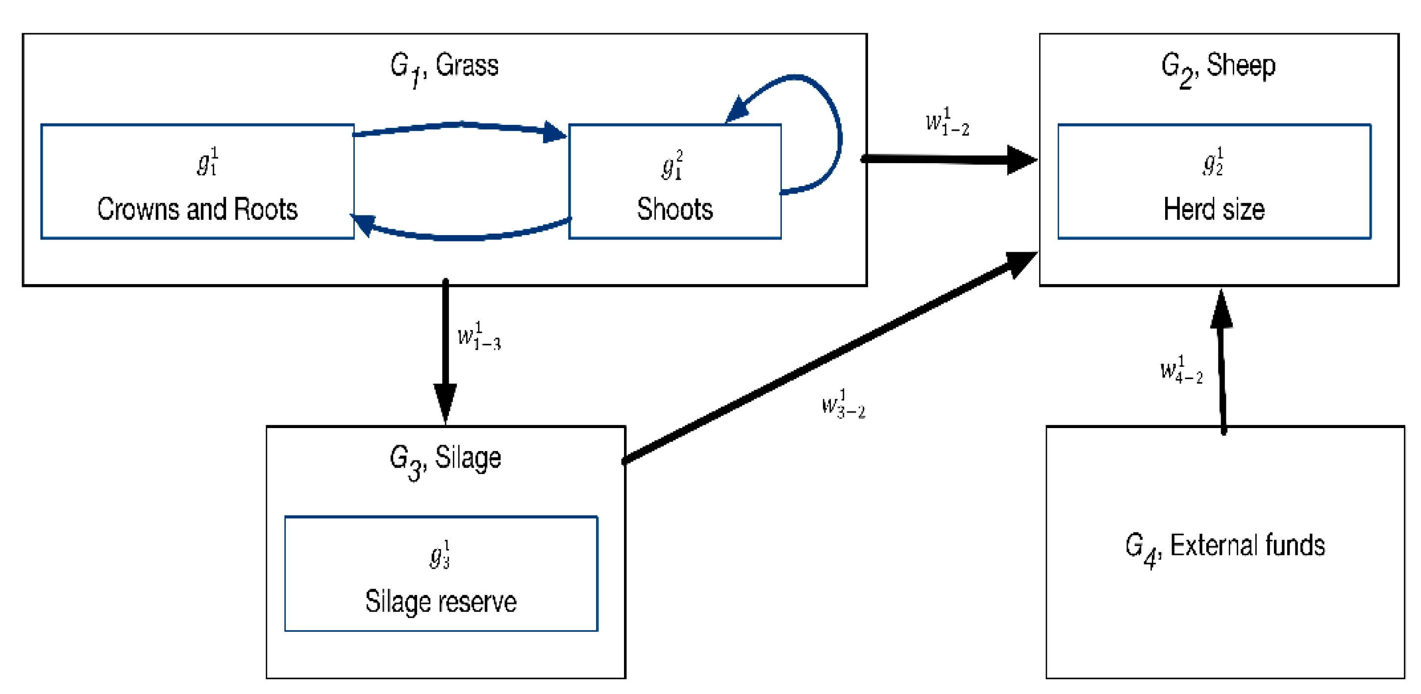
Figure 1. Sheep grazing management system model (funds, stock variables, and service flows). Note: the relation between variables within a fund, although represented in the figure, is only relevant and considered at a later modeling stage.
Sustainability 13 12408 g001
Figure 2. Grass system model (with internal variables and processes) (see [52]).
Sustainability 13 12408 g002
Figure 3. System dynamics (gray arrows representing state local variation) under shoot consumption pressure, γ g h = 0.54 : (a) S and C nullclines and variable variation (blue and cyan arrows), saddle and stable points; (b) system state separatrix and p1 to p4 initial state trajectories.
Sustainability 13 12408 g003
Figure 4. System dynamics (gray arrows representing state local variation) under shoot consumption pressure, γ g h = 0.73 : (a) S and C nullclines and variable variation (blue and cyan arrows), saddle and stable points; (b) system state separatrix and p1 to p4 initial state trajectories.
Sustainability 13 12408 g004
Figure 5. System dynamics (gray arrows representing state local variation) under shoot consumption pressure, γ g h = 0.81 : (a) S and C nullclines and variable variation (blue and cyan arrows), saddle and stable points; (b) system state separatrix and p1 to p4 initial state trajectories.
Sustainability 13 12408 g005
Figure 6. System realization with the SDE model with different “noise” intensity values. Realization parameters: r s = 4 , r c = 1, a c = 0.1, s ˜ = 0.6 , γ g h = 0.54 , initial state ( s o ,   c o ) = ( 0.45 ,   0.2 ) . (a) Realization variable values and density, for σ 1 =   σ 2 = 0.005 ; (b) realization variable densities in the C/S plane, for σ 1 =   σ 2 = 0.005 ; (c) realization variable values and density, for σ 1 =   σ 2 = 0.105 ; (d) realization variable densities in the C/S plane, for σ 1 =   σ 2 = 0.105 . Values for state variable S (C) are represented in red (blue) in (a,c) and along the x (y) axis in (b,d).
Sustainability 13 12408 g006aSustainability 13 12408 g006b
Figure 7. System realizations with the SDE model considering the same “noise intensity” values σ 1 =   σ 2 = 0.005 . Other realization parameters: r s = 4 , r c = 1, a c = 0.1, s ˜ = 0.6 , γ g h = 0.54 , initial state ( s o ,   c o ) = ( 0.2 ,   0.2 ) . (a) Variable values and density for Realization #27; (b) realization variable densities in the C/S plane for Realization #27; (c) variable values and density for Realization #33; (d) realization variable densities in the C/S plane for Realization #33. Values for the state variables S (C) are represented by the red (blue) line in (a,c) and x (y) axis in (b,d).
Sustainability 13 12408 g007aSustainability 13 12408 g007b
Figure 8. Quasi-potentials with realization parameters r s = 4 , r c = 1, a c = 0.1, s ˜ = 0.6 : (a) Quasi-potential for γ g h = 0.51 ; (b) quasi-potential difference between stable and saddle points for γ g h = 0.51 ; (c) quasi-potential for γ g h = 0.81 ; (d) quasi-potential difference between stable and saddle points for γ g h = 0.81 . (Note: the depicted negative values of C and S result solely from the computational algorithm used and have no correspondence to reality.)
Sustainability 13 12408 g008
Figure 9. Strong sustainability metric applied to the rangeland management system: (a) 3D view for the sustainability metric; (b) “Consumption pressure” projection; (c) “Epochs” projection; (d) details for the “Epochs” projection.
Sustainability 13 12408 g009
Figure 10. Biomass values in the rangeland agent-based model simulations. Light green color corresponds to high values of biomass; black color corresponds to very low biomass values; sheep’s locations are represented as white dots. (a) N = 35 sheep, 1 epoch; (b) N = 35 sheep, 5 epochs; (c) N = 35 sheep, 10 epochs; (d) N = 38 sheep, 1 epoch; (e) N = 38 sheep, 5 epochs; (f) N = 38 sheep, 10 epochs; (g) N=40 sheep, 1 epoch; (h) N = 40 sheep, 5 epochs; (i) N = 40 sheep, 10 epochs.
Sustainability 13 12408 g010
Figure 11. Crown/root and shoot biomass mean field evolution: (a) shoot biomass for N = 35 sheep; (b) crown/root biomass for N = 35 sheep; (c) shoot biomass for N = 38 sheep; (d) crown/root biomass for N = 38 sheep; (e) shoot biomass for N = 40 sheep; (f) crown/root biomass for N = 40 sheep.
Sustainability 13 12408 g011
Figure 12. “Rotation duration” of the current patch (in epochs) for different sheep population sizes.
Sustainability 13 12408 g012
Figure 13. Crown/root and shoot biomass mean field evolution for N = 38 sheep and extended time. (a) Shoot biomass; (b) crown/root biomass.
Sustainability 13 12408 g013
Table 1. Description of funds and stock variables in the sheep grazing management system model.
Fund ,   G u Stock   Variables ,   g u h
G 1 , grass
Rangeland grazed by sheep and harvested for silage.
g 1 1 , crowns and roots. Rangeland crowns’ and roots’ available biomass. Measured in dry matter (DM) kilogram equivalents available per unit area and epoch.
g 1 2 , shoots. Rangeland shoots’ available biomass. Measured in dry matter (DM) kilogram equivalents available per unit area and epoch.
G 2 , sheep
Herd to be raised.
g 2 1 , number of sheep. Herd, measured by the number of adult sheep in the herd.
G 3 , silage g 3 1 , silage reserve. Dry matter (DM) kilogram equivalents available from silage.
G 4 , external funds. External funds (e.g., dry pellets) that may need to be acquired for herd nutritional needs. Modeled in the simplified system as an inexhaustible fund, thus having no associated variables.
Table 2. Description of services and flows in the sheep grazing management system model.
Services ,   W j Flow   Variables ,   w x y j
W 1 , dry matter (DM) equivalents
Provision of the required dry matter equivalents in order to meet the herd’s feed requirements.
w 1 2 1 , grazing. Dry matter equivalents grazed by the herd. Measured in DM kilograms grazed per unit area and epoch.
w 1 3 1 , harvesting. Dry matter equivalents harvested for silage. Measured in DM kilograms harvested per unit area and epoch.
w 3 2 1 , silage consumption. Dry matter equivalents of silage consumed by the herd. Measured in DM kilograms consumed per epoch.
w 4 2 1 , external feeding. Dry matter equivalents of food from external sources (e.g., pellets) consumed by the herd. Measured in DM kilograms consumed per epoch.
Publisher’s Note: MDPI stays neutral with regard to jurisdictional claims in published maps and institutional affiliations.