Article

Correlation Analysis between Hydrologic Flow Metrics and Benthic Macroinvertebrates Index (BMI) in the Han River Basin, South Korea

1
Department of Civil, Environmental and Plant Engineering, Konkuk University, Seoul 05029, Korea
2
Division for Integrated Water Management, Korea Environment Institute, Sejong 30147, Korea
3
Division of Civil and Environmental Engineering, Konkuk University, Seoul 05029, Korea
*
Author to whom correspondence should be addressed.
Sustainability 2021, 13(20), 11477; https://doi.org/10.3390/su132011477
Submission received: 25 August 2021 / Revised: 12 October 2021 / Accepted: 14 October 2021 / Published: 17 October 2021
(This article belongs to the Special Issue Green Infrastructure and Resilient Stream Ecosystems)

Abstract

:
In aquatic ecosystems, flow is one of the most essential elements of aquatic species. It is necessary to explore the correlation with ecological indices for the management guidelines of aquatic ecosystems using flow because aquatic ecosystem data are limited. This study calculated the flow metrics using the flow and analyzed the correlation between the flow metrics and the ecological index. This study attempted to understand the correlation between the ecologic index and flow metrics. Flow metrics were quantified flow in various ways, depending on the size, frequency, and design of the flow. The characteristics of flow metrics were identified and the correlation with the ecological index was studied. The Pearson correlation coefficient values for 22 watersheds were compared using the flow data from 2008 to 2015 and the ecological index data from the BMI. In watersheds with high imperviousness, the Pearson correlation coefficient was negative, which indicated that the correlation in this study provides basic data for the quantitative evaluation of the river ecosystem by identifying the relationship between imperviousness and BMI. As a result, the highest Pearson correlation coefficient values of flow metrics were related to the flow coefficient of variation (MACV13-16; MHCV; MLCV).

1. Introduction

Healthy streams are highly valued by humans, as they offer a range of social benefits [1,2]. Additionally, the diversity of species is important because it is related to the health of streams and ecosystem services [3]. However, as human activities increase and development progresses, the health of rivers decreases. It has been commonly noticed that hydrologic alterations resulting from urbanization influence stream ecology. The elimination of riparian vegetation and the increase in imperviousness, which typically occur with urban development, gradually alter stream hydrology and aquatic ecosystems [1,3,4,5].
As an area becomes dominated by impervious surfaces, a shift in the distribution of water occurs from partial subsurface flow to nearly all surface runoff [6,7,8]. However, as the extent of impervious surfaces increases, the runoff response is amplified from increasingly smaller precipitation events [9]. Although it is important to accurately determine the arrangement and proportional amounts of different functional types of impervious surface cover, it is also critical to understand how geometric characteristics can affect relationships between components of the hydrologic cycle and ecology [8,10]. Lee et al. [11] examined the mediating effects of streamline geometry on the relationships between urban land use and the index of biological integrity (IBI) of the Nakdong River in Korea. Kim et al. [12] analyzed the relationship between green/urban areas and topographical variables with biological indicators using regression tree analysis, which considered spatial autocorrelation at two different scales. The benthic macroinvertebrate index (BMI) is a type of ecological index obtained from measurements of benthic macroinvertebrates [13].
Many researchers have focused on establishing methods of quantifying the health of watersheds. These studies show that the assessment of stream ecosystems can be quantified by using appropriate statistical techniques [14,15,16,17]. Olden and Poff [14] suggested more than 170 metrics, including the hydrologic alteration indicators that include at least 64 metrics that quantify changes in flow regime [15]. The more than 170 metrics explain the flow structure patterns, which, in conjunction with the physical environment, determine the physical processes that directly influence aquatic organisms. Many hydrologic flow metrics have been demonstrated to be helpful in relating the effects of urbanization to ecological measures [4,16,17,18].
Woo et al. [10] evaluated aquatic ecosystem health using water quality modeling results via the sequential wavelength assignment technique (SWAT) and random forest technique. They suggested that the aquatic ecosystem be investigated using data such as flow rate and river depth. Park et al. [19] characterized the Han River watershed in Korea and extracted key relationships among the watershed attributes and biological indicators of the streams. They used biological indicators of the streams to determine the biological status of the watershed and stream. Park et al. [19] analyzed the correlation between river morphological factors and water quality factors. Woo et al. [20] conducted a study on whether the flow affects water quality and aquatic health by simulating the flow using SWAT. When the flow increased, the aquatic health showed a tendency to increase [20]. Flow was expected as a factor for aquatic health [20]. However, only a few studies have performed correlation analyses and habitat suitability evaluations using flows with BMI to evaluate the aquatic ecosystem [20,21]. Thus, this study selects flow metrics from streamflow data and tries to understand the correlation between flow metrics and aquatic ecosystem. Flow metrics have been classified into magnitude flow, frequency flow, and design flow. A previous study quantified the flow in various ways according to the size, frequency, and design of the flow [22]. As a result, it is necessary to analyze the relationship between BMI and flow metrics.
The purpose of this study was to investigate the connection between imperviousness and ecological index by analyzing the correlation between imperviousness and the benthic macroinvertebrate index (BMI). Additionally, this study searched for strong correlations between hydrologic metrics and ecological indicators in the Han River basin, South Korea. The aim of this research was to determine the relationships between BMI and flow metrics and relationship between imperviousness and BMI. A correlation analysis was conducted with the ecological index of BMI using 67 flow metrics. Figure 1 illustrates the process of the watershed selection and research. This study selected watersheds in the following order (Figure 1), and the corresponding flow metrics were calculated and compared with BMI, the representative ecological index.

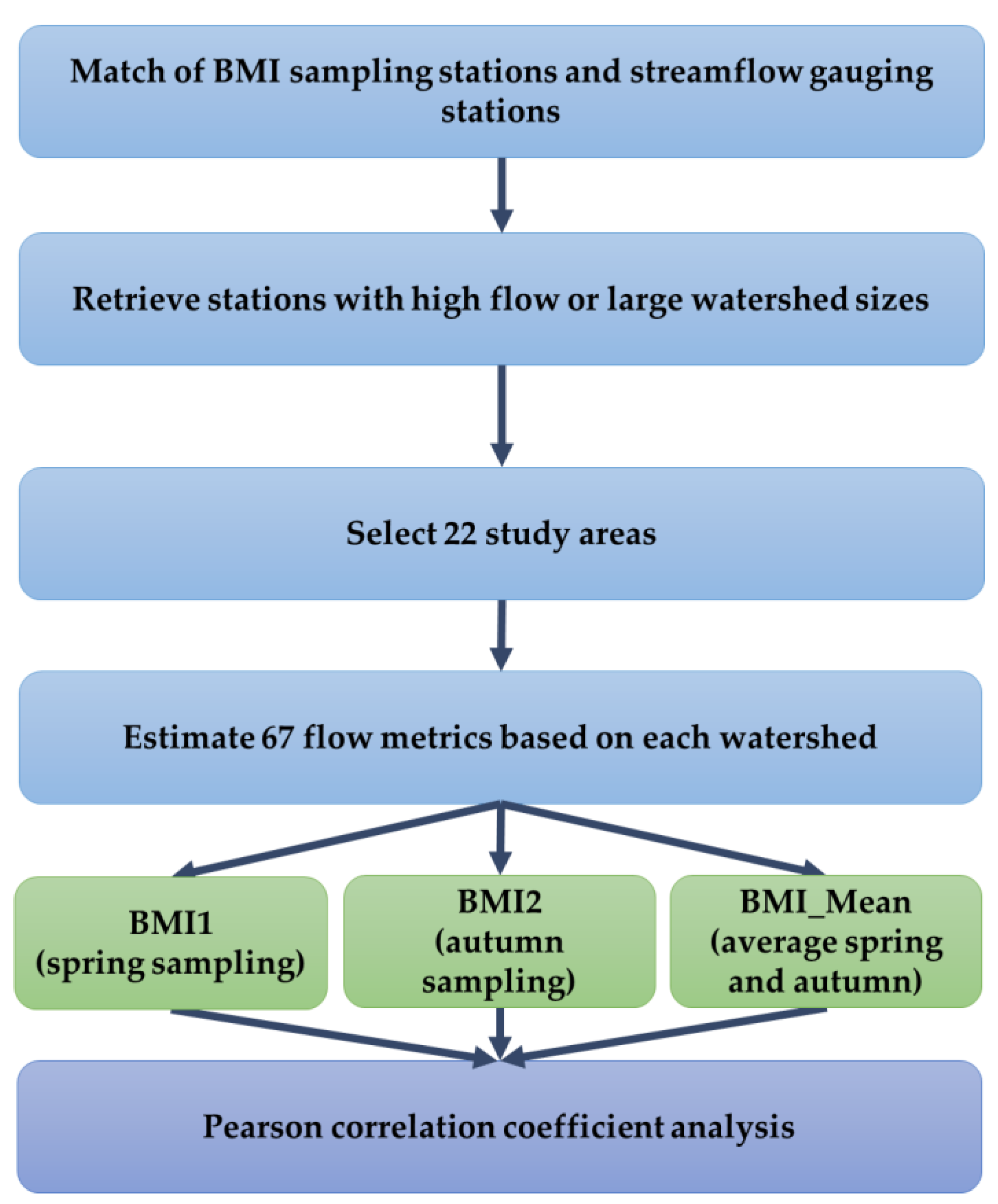
2. Materials and Methods
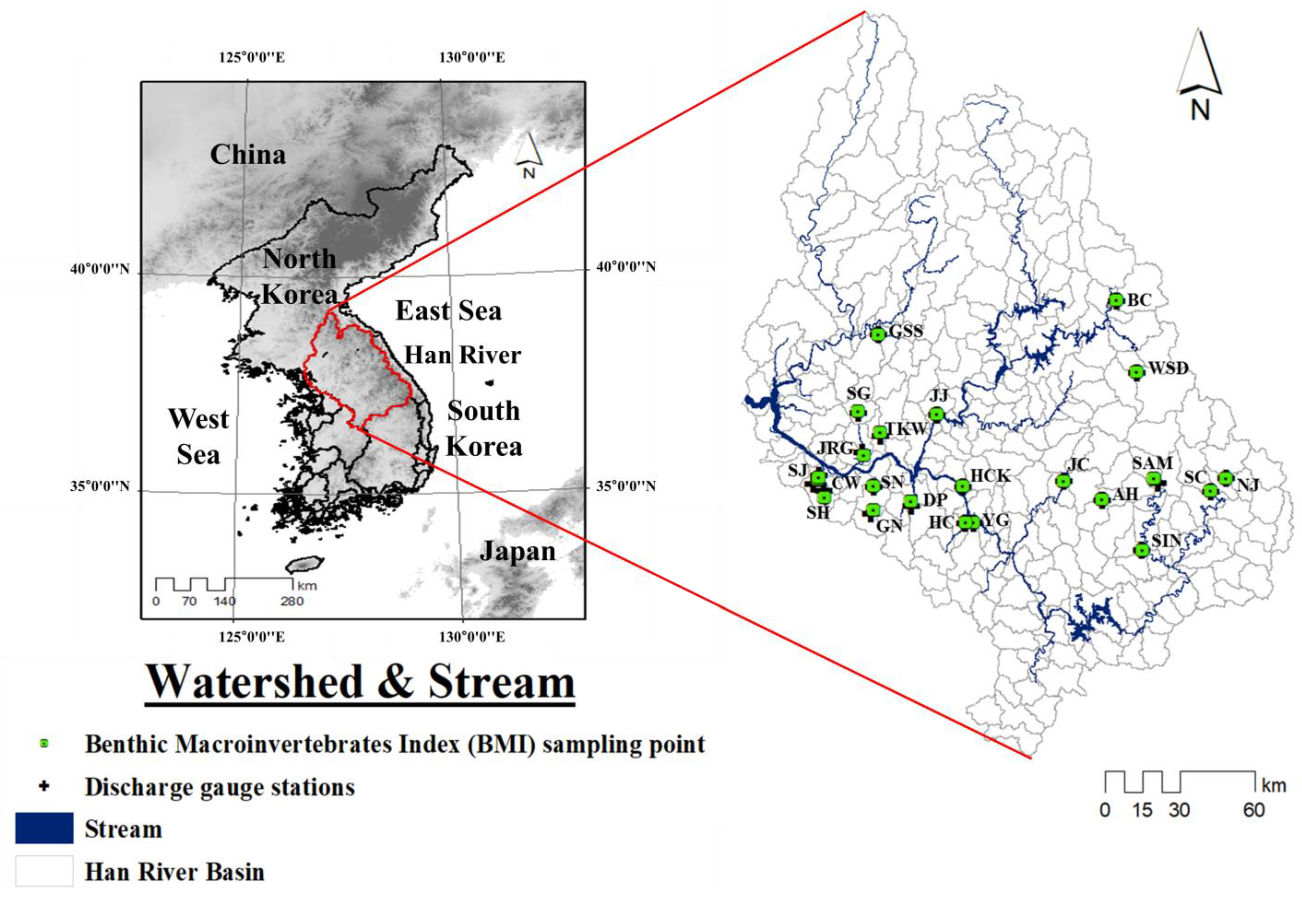
2.1. Study Area

This study focuses on the Han River basin (32,971 km2), one of the five major river basins (99,720 km2) in South Korea. This basin covers approximately a quarter of the country and is located from 36.03° N to 38.55° N and 126.24° E to 129.02° E (Figure 2). The North Han River (10,652 km2) and the South Han River (12,514 km2) are the two major rivers in the basin, which merge and flow into Seoul, a metropolis of ten million people [23]. This country’s climate is characterized by four seasons, with heavy precipitation occurring during the monsoon summer season (June to August) [24]. The average annual precipitation is 500~1500 mm, which results in a relatively wet climate. The seasonal distribution of precipitation is not uniform, and the wet and dry seasons are distinct. Most of the annual precipitation is concentrated in the summer, with very little during the winter (Korea Meteorological Agency, (KMA)). The average elevation of the Han River basin is 404.7 m, and the average slope of the basin is 35.9% [25]. This study used land use data in 2008 (Table 1). The watershed land use consisted of urban areas (8.2%), forested areas (71.3%), agricultural land (16.6%), and other land uses (3.9%). Two soil types presented with 58% sandy loam and 24% loam are dominant in Han River basin [10]. The seasonal variations in air temperature for spring, summer, fall, and winter were 10.8 °C, 23.6 °C, 12.6 °C, and −2.9 °C, respectively [10].
Although the Han River basin is divided into 237 subcatchments, streamflow monitoring and BMI sampling have not been performed in all subcatchments [13]. Therefore, we selected the test area based on the following criteria: (1) watersheds with watershed areas less than 1000 km2, (2) watersheds with BMI data provided by Water Environment Information System (WEIS, http://water.nier.go.kr; accessed on 12 October 2021), and (3) watersheds with daily flow data, daily water level data and rating curve equations provided by Water resources Management Information System (WAMIS) (http://www.wamis.go.kr; accessed on 12 October 2021). Thus, a total of 22 watersheds were designated as study watersheds (Table 1). Imperviousness is one of the indicators that expresses urban characteristics. The percent imperviousness is calculated based on the ratio of urban area to total watershed area as following equation and is expressed as % in Table 1.
imperviousness   ( % ) = Urban   area Total   area × 100

2.2. Description of Hydrological Flow Metrics

The flow metrics were classified by the magnitude of the flow, including the average flow, maximum flow, and minimum flow [15,17,26,27,28,29,30]. Additionally, the flow metrics were categorized with the frequency and variability in the flow (Table 2) [15,17,26,27,30,31]. The flow metrics that are used for river planning and design in Korea include flood flow (Q10), abundant flow (Q95), ordinary flow (Q185), low flow (Q275), and drought flow (Q355) [32,33,34]. The corresponding flow metrics are flow values that are designed not to fall below the flow corresponding to the number of days during river planning and design. This study conducted a comparative analysis of BMI (the ecological index) and these flow metrics (hydrologic variables) (Table 2).
The flow metrics were calculated from daily flow data of the watersheds from 2008 to 2015. For watershed without observations, we calculated daily flows with the rating curve equations by Water resources Management Information System (WAMIS) (http://www.wamis.go.kr; accessed on 12 October 2021). The observed daily flow data were partially provided by WAMIS for the Sinjeong (SJ), Jungranggyo (JRG), Sihueng (SH), Seongnam (SN) and Singok (SG) watersheds. Other watersheds were described with daily flows calculated by the rating curve equations provided by WAMIS.

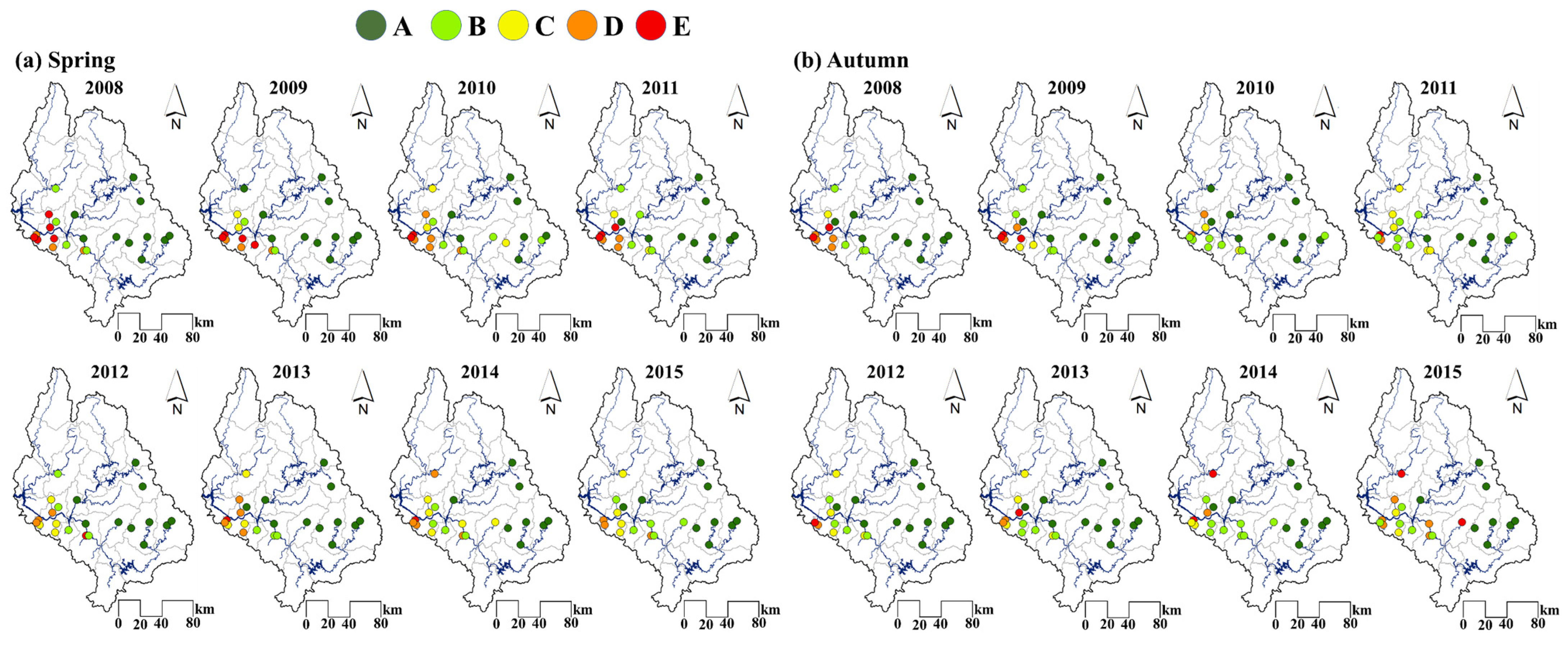
2.3. Benthic Macroinvertebrates Index (BMI)

The benthic species referred to here are invertebrates living in the riverbed, such as aquatic insects, shellfish, crustaceans, and leeches. Benthic species are one of the most important ecological and environmental indicators [21]. BMI is the most commonly used index in aquatic environment assessments. BMI is divided into five grades, A–E (Table 3), as follows [10,21,35].
BMI = ( 4 i = 1 n s i h i g i i = 1 n h i g i ) × 25
where BMI = benthic macroinvertebrate index, i =   the   number   assigned   to   the   species , n =   the   number   of   species , s i =   the   saprobic   value   of   species   i , h i =   the   relative   abundance   of   species   i , and g i =   the   indicator   weight   value   of   the   species   i , The appearance, saprobic value and the indicator weight value of the species from nearly 190 categorizations were used to estimate BMI based on the method suggested by Zelinka et al. [36]. Kong et al. [35] reported that BMI was a more capable index of assessing stream health and integrity when utilizing relative abundance information.
The distribution of BMI class in the study area in spring and autumn were determined at monitoring points, as shown in Figure 3. A significant difference by year was shown in low BMI classes (D and E) but was not present in high BMI classes (A and B). In the spring season (Figure 3a), the difference in class by watershed was larger than that in the fall season (Figure 3b). The BMI values were used as the observed data from 2008 to 2015. BMI was sampled twice during the spring and autumn seasons. The BMI values were classified into primary and secondary values. Spring and autumn have more stable environmental conditions than summer and winter, so the corresponding data are suitable for this investigation. In the case of rainfall during the investigation, it is customary to stop the investigation and restart after more than 10 days have elapsed. Additionally, the one-month period following a flood was excluded from the investigation period. The survey period varied according to the weather during the sampling period. In this study, the BMI values used were the first, second, and average values [13,37]. The first BMI values were collected in the spring. The second BMI values were collected in the autumn. Additionally, the average of the first (spring) and second (autumn) values was used in this study. The first (spring) BMI value is expressed as BMI1, the second (autumn) BMI value is expressed as BMI2, and the average BMI value is expressed as BMI_Mean.

2.4. Pearson’s Correlation Coefficient Analysis

The Pearson product-moment correlation coefficient is a dimensionless index that remains unchanged when either component is transformed linearly. In 1895, Pearson devised the mathematical formula for this essential metric.
r = ( X i X ¯ ) ( Y i Y ¯ ) [ ( X i X ¯ ) 2 ( Y i Y ¯ ) 2 ] 1 / 2
where X i = flow metric values, Y i = BMI values, X ¯ = mean flow metric values, and Y ¯ = mean BMI values.
The correlation coefficient, which ranges from −1 to 1, is a measure of how closely variables are related to each other. There is no linear relationship if r = 0. A perfect positive or negative linear relationship occurs if r = −1 or 1 [38,39].
This metric is the measure of the association between the change trends for each pair of corresponding variables. The Pearson correlation coefficient assesses the similarity between shifts in two variables. Additionally, this coefficient tests the intensity of the linear relationship between two variables [40]. MATLAB (MathWorks Inc., Natic, MA, USA) was used to calculate the Pearson correlation coefficients. A 5% significance level was considered (p-value < 0.05).

3. Results

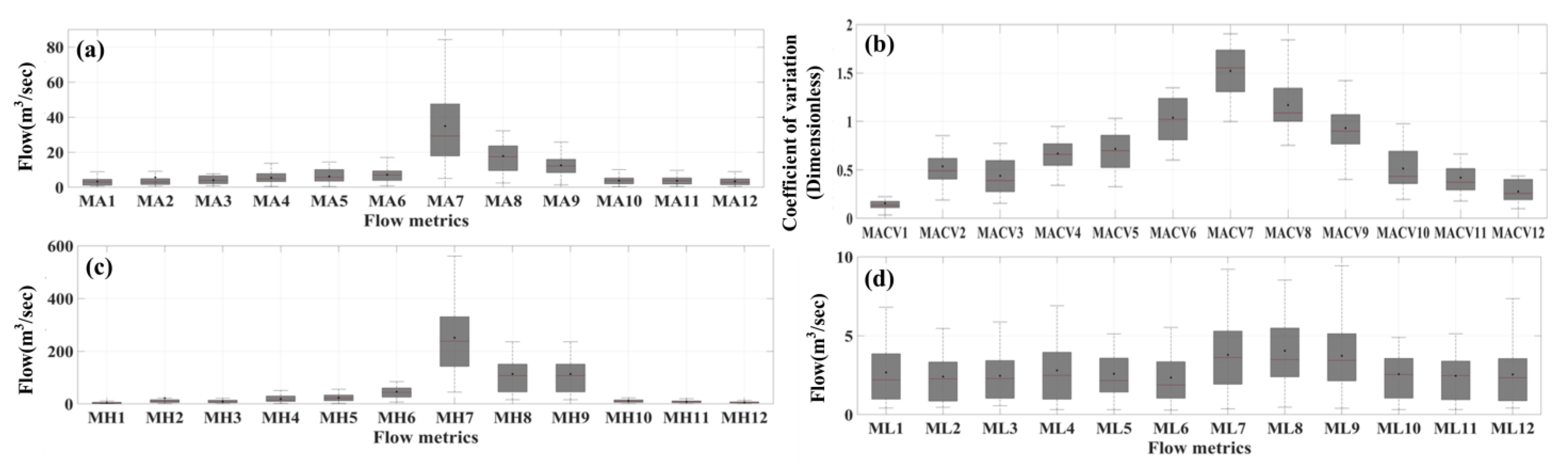
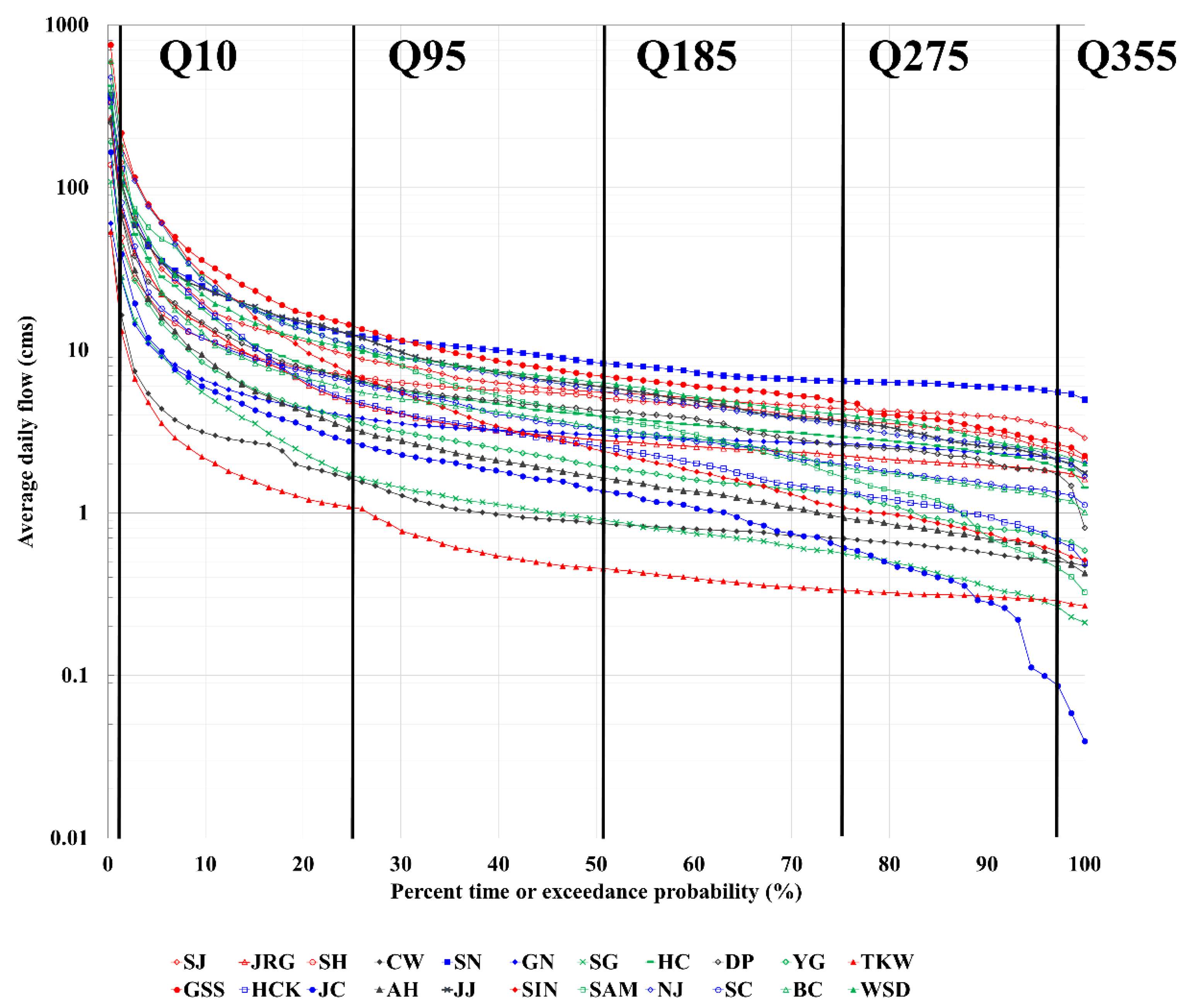
3.1. Calculation Results of Flow Metrics

Flow metrics were calculated for each watershed. According to the characteristics of flow, the metrics are largely classified into magnitude, frequency, and design flow metrics. A box plot of magnitude flow metrics was used to identify the relationship between flow and flow metrics. Figure 4a–d illustrate the values of the magnitude flow metrics. The flow metrics in Figure 4a–d were calculated using the monthly and daily flows (MA1-12, MACV1-12, MH1-12, and ML1-12). MA1-12 and MACV1-12 indicate the flow characteristics of each month in terms of the mean monthly daily flow (January–December) and variability in monthly flow (January–December). Korea has a monsoon climate, and the rainfall is concentrated in summer [24]. The flow is high in the summer when there is concentrated rainfall [24]. MA7-8 and MACV7-8 have the largest ranges in Figure 4a,b and thus indicate the characteristic of concentrated rainfall in summer. Figure 4c,d present the maximum daily flow (January–December) and minimum daily flow (January–December) as box plots. MH7 represents the largest range in Figure 4c. MH4-6 presents a similar range distribution. The ML1-12 results illustrate the homogeneous data ranges in Figure 4d.
Figure 5 illustrates the flow duration curve (FDC) and design flow metrics for each watershed. This study used an FDC to evaluate the streamflow processes. An FDC, also known as a percent exceedance probability curve, is a graphical tool to describe streamflow [41]. The values of the FDC are different for each watershed in Figure 5. The shape of an FDC is affected mainly by reservoirs, land use type, and upstream water use at a daily scale [41]. Watersheds with higher imperviousness had a larger FDC, as shown in Figure 5. This indicated that land use influenced the FDCs. The watershed with the largest flow value was SN, and the watershed with the smallest value was JC, as shown in Figure 5. In particular, the difference in FDC values between watersheds increased as the flow approached Q355 (the drought flows).

3.2. Correlation Analysis between Hydrological Compoenet and BMI

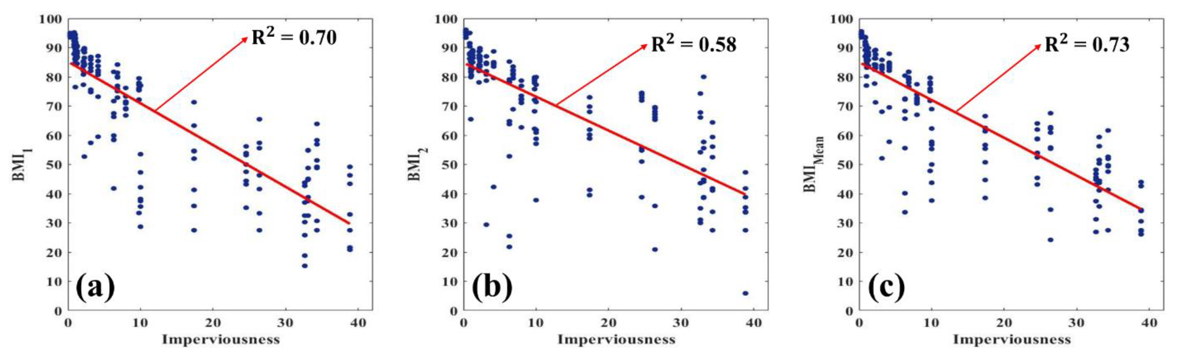
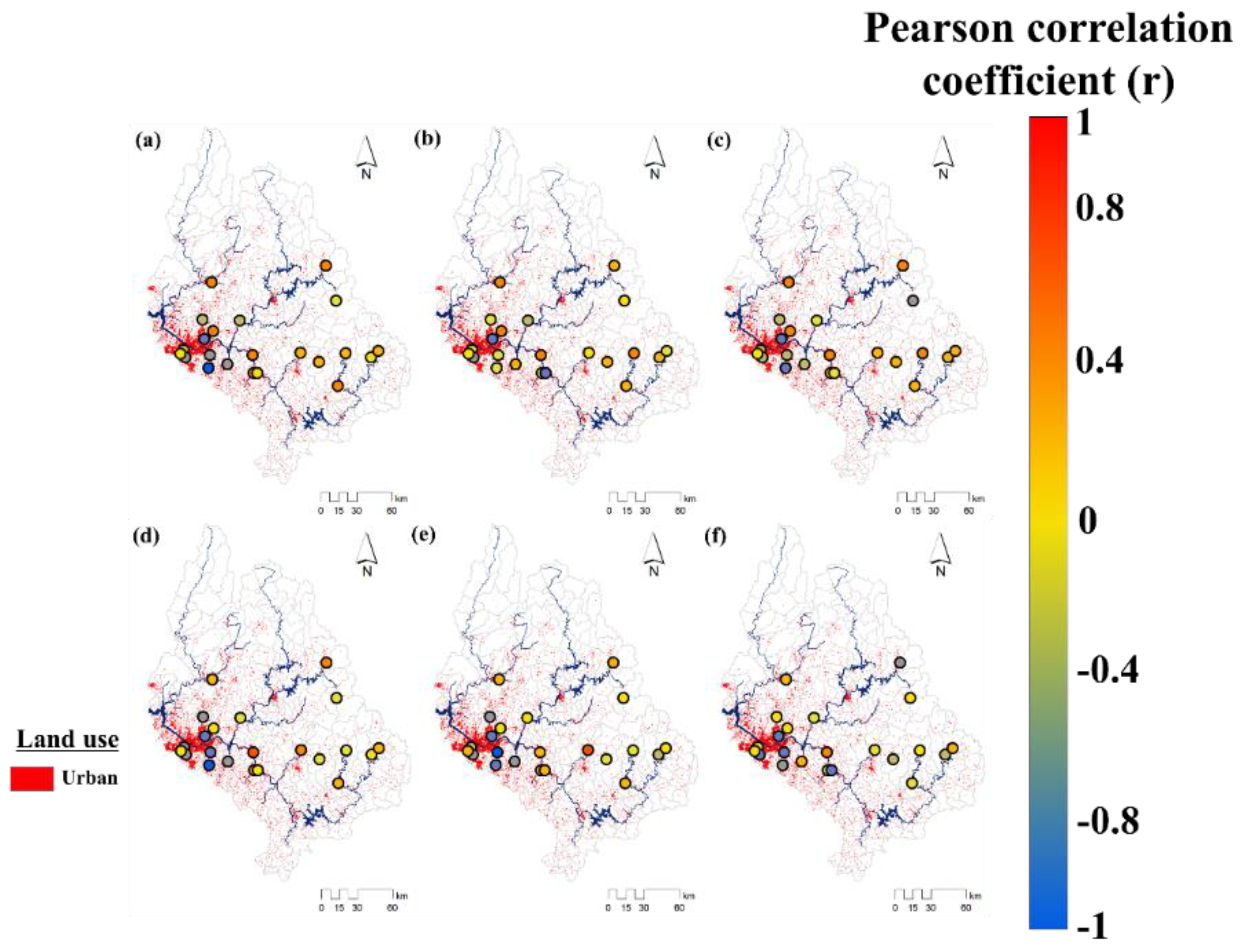
3.2.1. Relationship between Imperviousness and BMI

Figure 6 indicates the results of the imperviousness and BMI. As imperviousness increases, the BMI values decrease. In particular, relatively high R 2 values are obtained from the BMI primary value (a) and the average value (c), and there are correlations between the imperviousness and BMI values. The BMI decreases as imperviousness rises in Figure 6, suggesting a negative relationship between imperviousness and BMI. However, the prediction of biological conditions at a given location does not depend on the imperviousness of the watershed alone [18]. The imperviousness is also connected to flow. Surface runoff increases as imperviousness increases, and the discharges that flow quickly into the river continue to increase [42]. This study identified the correlation between flow and BMI by conducting a Pearson correlation analysis between flow metrics and BMI.

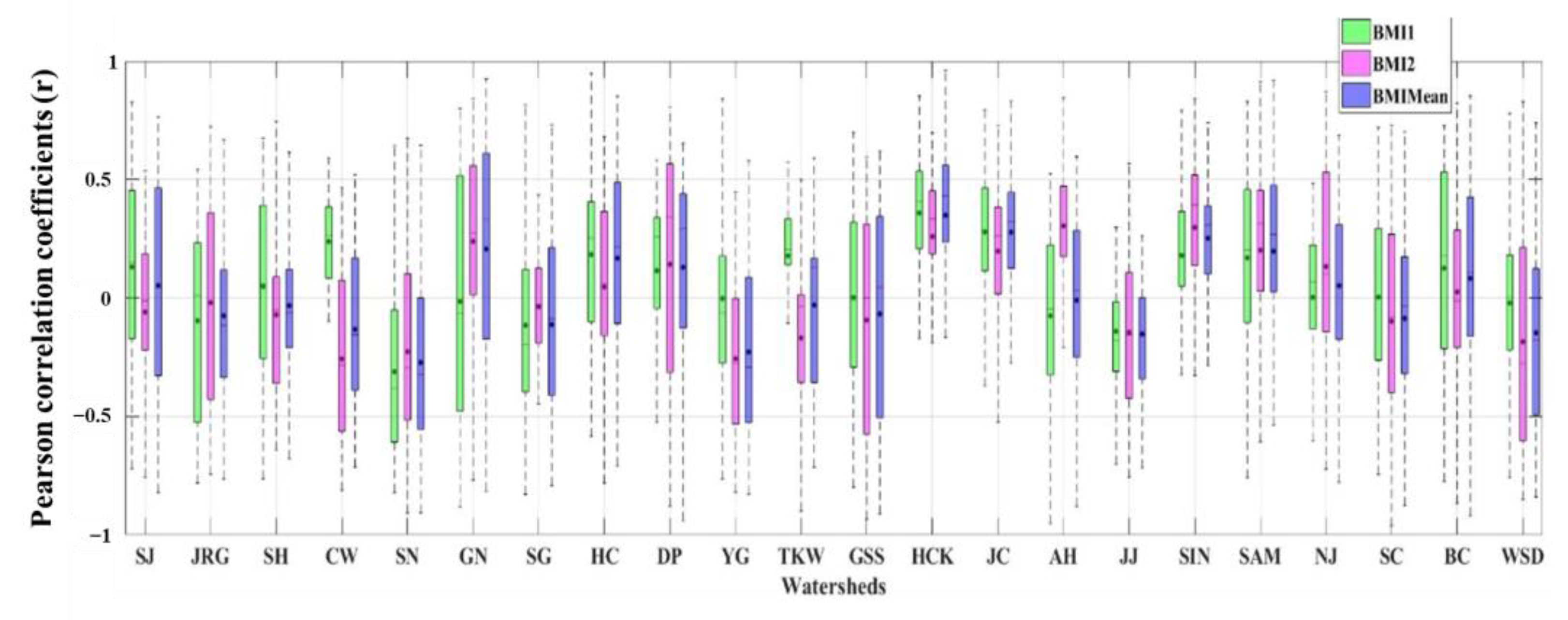
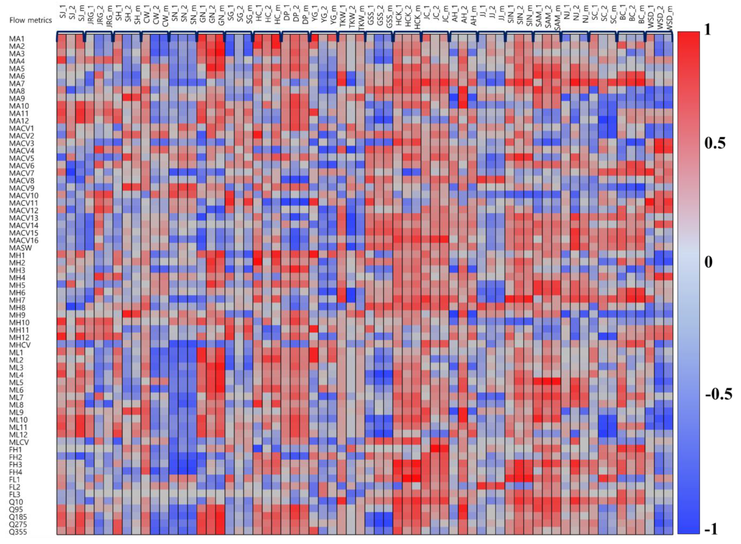
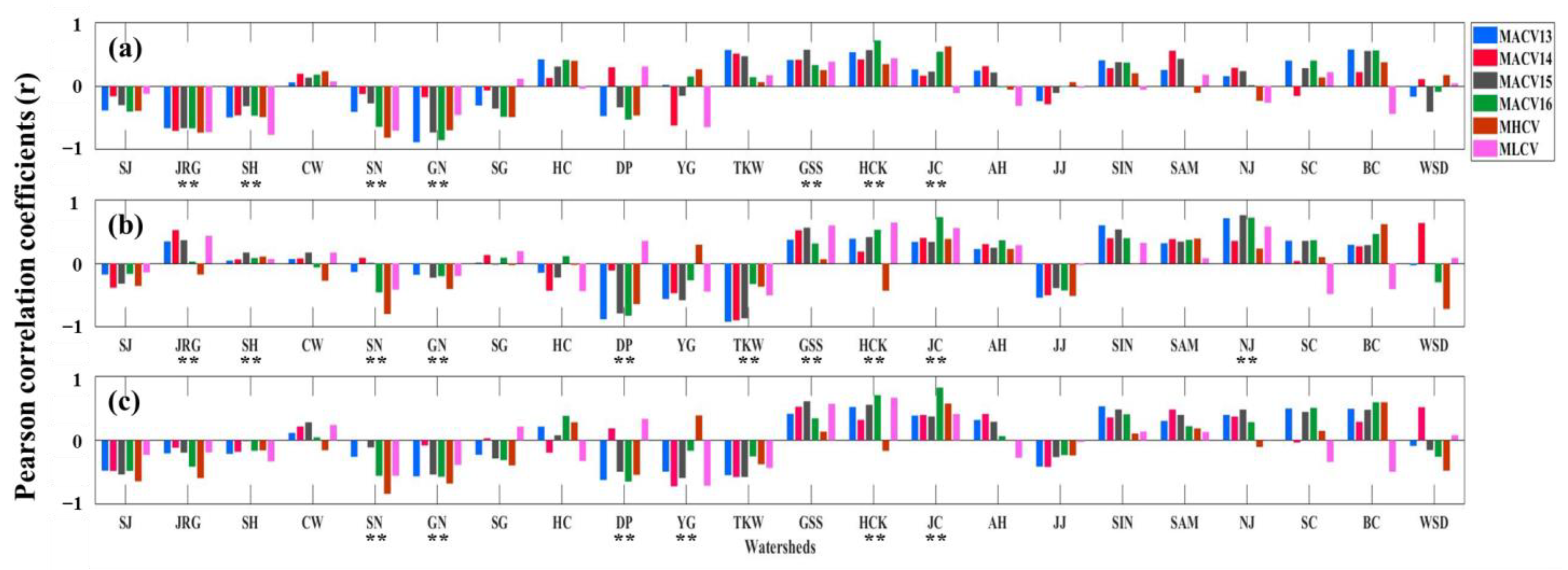
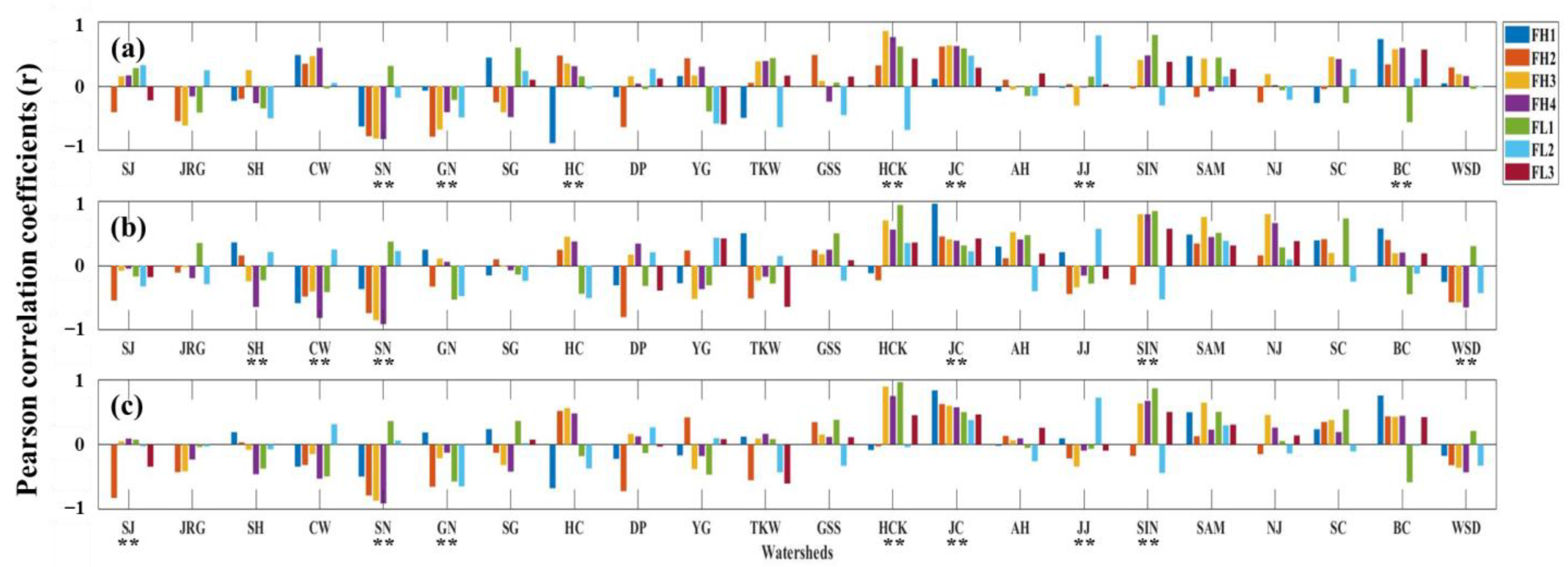
3.2.2. Correlation Analysis between Flow Metrics and BMI

This study conducted a Pearson correlation analysis between flow metrics and BMI to describe the correlations. Figure 7 illustrates the box plot result of the Pearson’s correlation coefficient analysis. This box plot confirmed the range of correlation coefficient values for the studied watersheds. In the boxplot, the IQRs (i.e., 25~75th quantiles) are represented by boxes, the whiskers extended to the 5th and 95th quantiles, and the red horizontal line indicates the median [43]. The Pearson coefficient obtained with BMI2 in Figure 7 represents a larger data range than those obtained with BMI1 and BMI_mean. Pearson coefficients obtained with BMI1 and BMI_Mean have similar IQRs. Figure 7 demonstrates that the Pearson correlation coefficient values are distributed in various ranges. Each watershed has different correlations to the flow metrics, and each watershed has a negative correlation and a positive correlation among the different flow metrics. Most watersheds have different correlations with BMI, but some watersheds have similar results. Watersheds such as SN, SG, HCK, JC, and SIN illustrated analogous data ranges in Figure 7.
The SN watershed illustrates negative correlation data ranges in Figure 7. The HCK and JC watersheds have very small data ranges. In addition, the Pearson correlation coefficient values between the HCK and JC watersheds suggest positive correlations. The TKW watershed has positive correlations with BMI1. However, in the TKW watershed, the data ranges of the Pearson correlation coefficient values in BMI2 and BMI_Mean were large. Most of the Pearson correlation coefficient values obtained between BMI1, BMI2, and BMI_Mean and the flow metrics for each watershed were similarly distributed. However, the SJ, JRG, SH, CW, NJ and WSD watersheds show differences in their data ranges, as illustrated in Figure 7.
Figure 8 shows the correlation analysis results for the 67 flow metrics and BMIs for 22 subwatersheds as a heatmap. In the figure, red indicates a positive correlation between the flow metrics and BMI values, and blue indicates a negative correlation. Terms such as SJ_1, SJ_2, and SJ_m in the upper part of Figure 8 indicate the Pearson correlation coefficient values for each watershed using the flow metrics and BMI1(1), BMI2(2), and BMI_Mean(m).
Overall, most of the watersheds with low imperviousness illustrated positive correlations (e.g., GSS, HCK, JC, SIN, and SAM). BMI1, BMI2, and BMI_Mean consistently exhibit positive correlations, as shown in Figure 8. The frequency-related flow metrics represent negative correlations in the watersheds with high imperviousness and positive correlations in the watersheds with low imperviousness. The flow metrics related to coefficients of variation of magnitude flow exhibit a negative correlation in the watersheds with high imperviousness.
In particular, the flow index related to magnitude showed clear trends (MA1-12, MACV1-12, MACV13-16, MH1-12, ML1-12, MHCV and MLCV). MACV13-16 exhibit significant differences among watersheds according to imperviousness. The MACV13-16 flow metric values indicate a negative correlation with BMI of watersheds with high imperviousness. The correlation analysis values of the flow metrics and BMI present a positive correlation in the watersheds with low imperviousness. This suggests that the imperviousness of the watershed has an indirect effect on the flow and the ecological index BMI [12]. The SN watershed exhibits negative correlations for all 67 flow metrics. Negative correlations were also found for MHCV, ML1-12, and FH1-4. HCK exhibits a positive correlation for all 67 flow metrics. Overall, a positive correlation was generally found for FH3-4 and FL1.
On the other hand, BMI1 and BMI2 show different correlation analysis results in different measurement seasons. Choi et al. [44] stated that the rainfall characteristics of Korea, where rainfall is concentrated in summer, also affect the aquatic ecosystem. Concentrated rainfall during the summer results in the dilution of organism density in ecosystems by augmenting water levels or discharge [44,45,46]. BMI1 was monitored before summer rainfall, and BMI2 was collected after summer rainfall. BMI2 indicates significantly lower scores than BMI1 in terms of the pattern and collection results. BMI2 values without a pattern act as a factor indicative of inconsistent characteristics in the correlation analysis. BMI2 values generally illustrate different correlations between watersheds in Figure 8. In the SG watershed, the Pearson correlation analysis results between the BMI1, BMI2, BMI_Mean values and flow metrics exhibit a large difference between BMI1 and BMI2. In the SG watershed, the correlations between the flow metrics and BMI values are low, but the correlation results between BMI1 and BMI2 are different. In particular, the correlation analysis results (SG_2) of BMI2 in the SG watershed show no correlation for most flow metrics. The correlation analysis results in the TKW watershed also differed between BMI1 (TKW_1) and BMI2 (TKW_2). MACV12-16 and BMI1 (TKW_1) in the TKW watershed exhibit positive correlations. However, MACV12-16 and BMI2 (TKW_2) in the TKW watershed have negative correlations.
This analysis identified correlativity among flow metrics and BMI. Figure 9, Figure 10 and Figure 11 represent the correlation results for each flow metric type. Figure 9 demonstrates the results of the Pearson’s correlation analysis between the BMI values and flow metrics in terms of the coefficient of variation. Six watersheds (SJ, JRG, SH, SN, GN, and SG) illustrate almost negative correlations among the flow metrics in terms of the coefficient of variation in Figure 9. In the correlation analysis between the BMI1 index and MACV13, the seven basins with the last highest imperviousness produce negative correlations, excluding the CW watershed. The JRG watershed and GN watershed exhibit high negative correlations of −0.66 and −0.88, respectively, for MACV13 in Figure 9a. BMI2 and flow metrics related to coefficient of variation values indicate no correlation in the watersheds with a high imperviousness, as shown in Figure 9b. The BMI1 and BMI_mean represent similar correlation results in Figure 9a,c.
Figure 10 presents the results of the correlation analysis between the flow metrics obtained using the frequency flow metrics and BMI values. Although the frequency indices FH1-4 and FL1-3 are weakly correlated to the BMI values, they exhibit negative correlations in a watershed with high imperviousness and positive correlations in a watershed with low imperviousness. FH2 has a strong negative correlation in the SN and GN watersheds in Figure 10a,c and a positive correlation in the HCK watershed. However, the correlation strengths of FH2 are lower than those of the MACV flow metrics in Figure 9, for each watershed. The FH flow metric of high flow frequency index is more correlated with the ecological index than the FL flow metrics (the low-flow frequency index).
Figure 11 indicates the results of the correlation analysis between the flow metrics obtained using the design flow metrics and the BMI values. The SN watershed exhibits negative correlations for BMI1, BMI2, and BMI_Mean, as shown in Figure 11a–c, respectively. In the GSS watershed, negative correlations were found in Q185, Q275, and Q355, but not Q10 and Q95, as shown in Figure 11a–c, respectively. BMI1 represents a positive correlation, but BMI2 and BMI_Mean present negative correlations in Figure 11. However, the correlation between the design flow metrics and ecological index BMI was low in most watersheds.
Figure 12 illustrates the spatial patterns of the Pearson correlation coefficient between the BMI1 values and flow metrics regarding the coefficient of variation (MA13-16, MHCV, MLCV). This study does not consider land-use changes over time due to the limited land use change data (Table 1). It was found that the corresponding Pearson correlation coefficient value represented a negative correlation to the west region on the map for the watershed with high spatial imperviousness. In addition, the watershed located to the east region showed a positive correlation with the Pearson correlation coefficient as the watershed with a low imperviousness.

4. Discussion

This study analyzed the correlation between flow metrics and BMI, as a representative ecological index. This study calculated the flow metrics using calculated flows from rating curves. The coefficient of variation is often used to check the deviation, rather than the difference in the absolute values [47]. This study found that most watersheds illustrated similar correlations according to the coefficient of variation. Thus, the variability in flow affects the BMI. The correlation was low for the frequency flow metrics in Figure 10. The high flow frequency was more highly correlated with BMI than the low flow frequency. This indicates a greater correlation with BMI at high flows [48,49]. Unlike previous studies [14,49,50], this study did not compare combined flow metrics. However, this study analyzed the correlation between flow metrics and BMI. Through this correlation analysis, it was possible to identify which flow metrics were correlated with BMI. In most cases, when analyzing the correlation with BMI, the water quality factor or flow is used [21]. However, this study adjusted different flow values for each watershed by processing and analyzing the flow into different flow metrics. This study suggested basic data to quantitatively evaluate river health through correlation analysis between flow metrics and BMI.
The flow metric values identified differences according to the rainfall characteristics in Figure 4. Precipitation is one of the important climatic characteristics of Korea. The average annual precipitation is 500–1500 mm, which results in a relatively wet climate. The seasonal distribution of precipitation is not uniform, and the wet and dry seasons are distinct. Most of the annual precipitation is concentrated in the summer, with very little during the winter KMA). Korea has a concentrated rainfall pattern in summer [44,45]. The characteristics of this rainfall pattern can be seen in the flow metrics. Through the analysis of the value distribution and range of the flow metrics, flow characteristics were identified (Figure 4a–d). The ranges, averages, median values, and IQRs of the flow metrics in Figure 4 indicate which flow metrics have the largest data ranges. It was found that the larger the flow metric values within the data ranges in Figure 4, the lower the correlation with the BMI values in Figure 8 (e.g., MA7-8 and MH7-8).
By comparing the imperviousness and BMI of the land, it was found that BMI tends to decrease when imperviousness increases. However, BMI2 represented a lower correlation than BMI1 and BMI_Mean. This finding is due to environmental differences resulting from the unique climate of Korea, where rainfall is largely concentrated in summer [44,45,46]. The imperviousness and BMI values had a negative correlation. In other words, this finding suggests that imperviousness affects BMI. Numerous researchers have found that imperviousness affects river ecosystems [14,18]. This trend was similar to those presented in other studies [1,18]. Figure 7 illustrates the range of Pearson correlation coefficient values for each watershed. According to the BMI1, BMI2, and BMI_Mean results for each watershed, the data distributions were similar, but the data ranges were different in some watersheds due to the seasonal difference in the BMI and the differences in flows. Thus, the top seven watersheds with high imperviousness corresponded to a negative correlation in terms of the Pearson’s correlation coefficient values, and a lower imperviousness corresponded to a positive correlation. In particular, these correlations were strong according to the coefficient of variation, as shown in Figure 9.

5. Conclusions

In this study, 67 flow metrics were calculated and evaluated for each selected watershed, and the corresponding BMI was compared. In addition, correlation analyses of these metrics and ecological index were performed for each watershed via Pearson’s correlation coefficient analysis, and correlations were found. As a result, in the case of a watershed with high imperviousness, the correlation analysis between the flow metrics and the ecological index BMI had negative Pearson correlation coefficients. This study found that if imperviousness increases, BMI decreases, and these data show that the flow of the watershed is also affected. This study quantitatively presented the flow metrics of the watersheds. This study attempted to present basic data for quantitatively calculating river health in a watershed using BMI, which is one of the quantitative ecological indices. This study identified the correlation between the 67 flow metrics and BMI for each watershed and confirmed that the flow metrics estimated by the coefficient of variation produces stronger correlations with BMI than other flow metrics. The flow metrics can be used to establish a plan to improve aquatic health. If research in the entire Han River basin is conducted using these data in the future, it will be more helpful in evaluating river health. Significant correlations were identified for each watershed, but correlation analysis for the larger scale, the entire Han River basin, was insufficient. Thus, it is believed that future studies can obtain more meaningful results if correlation analyses are performed on the flow metrics and BMI in the entire Han River basin using machine learning.

Author Contributions

Conceptualization, S.K. (Siyeon Kim) and D.P.; funding acquisition, D.P.; data curation and investigation, S.K. (Siyeon Kim), J.L., S.J., M.L., H.A. and K.J.; methodology, S.K. (Siyeon Kim), J.L., S.K. (Seongjoon Kim) and D.P.; software, S.K. (Siyeon Kim); supervision, D.P.; writing—original draft, S.K. (Siyeon Kim); writing—review and editing, S.K. (Seongjoon Kim) and D.P. All authors have read and agreed to the published version of the manuscript.

Funding

This paper received no external funding.

Institutional Review Board Statement

Not applicable.

Informed Consent Statement

Not applicable.

Data Availability Statement

The data presented in this study are available on request from the corresponding author.

Acknowledgments

This study was supported by Konkuk University in 2020.

Conflicts of Interest

The authors declare no conflict of interest.

References

  1. Booth, D.B.; Jackson, C.R. Urbanization of Aquatic Systems: Degradation Thresholds, Stormwater Detection, and the Limits of Mitigation. J. Am. Water Resour. Assoc. 1997, 33, 1077–1090. [Google Scholar] [CrossRef]
  2. Meyer, J.L. Stream Health: Incorporating the Human Dimension to Advance Stream Ecology. J. N. Am. Benthol. Soc. 1997, 16, 439–447. [Google Scholar] [CrossRef] [Green Version]
  3. Paul, M.J.; Meyer, J.L. Streams in the urban landscape. Annu. Rev. Ecol. Syst. 2001, 32, 333–365. [Google Scholar] [CrossRef]
  4. Konrad, C.P.; Booth, D.B. Hydrologic Changes in Urban Streams and their Ecological Significance. Am. Fish. Soc. Symp. 2005, 47, 17. [Google Scholar]
  5. Roy, A.H.; Freeman, M.C.; Freeman, B.J.; Wenger, S.J.; Ensign, W.E.; Meyer, J.L. Investigating Hydrologic Alteration as a Mechanism of Fish Assemblage Shifts in Urbanizing Streams. J. N. Am. Benthol. Soc. 2005, 24, 656–678. [Google Scholar] [CrossRef]
  6. Putnam, A.L. Effect of Urban Development on Floods in the Piedmont Province of North Carolina; US Geological Survey: Raleigh, NC, USA, 1972.
  7. Johnson, S.L.; Sayre, D.M. Effects of Urbanization on Floods in the Houston Texas Metropolitan Area; US Geological Survey, Water Resources Division: Austin, TX, USA, 1973; Volume 3.
  8. Shuster, W.D.; Bonta, J.; Thurston, H.; Warnemuende, E.; Smith, D.R. Impacts of Impervious Surface on Watershed Hydrology: A Review. Urban Water J. 2005, 2, 263–275. [Google Scholar] [CrossRef]
  9. Sheeder, S.A.; Ross, J.D.; Carlson, T.N. Dual urban and rural hydrograph signals in three small watersheds 1. JAWRA J. Am. Water Resour. Assoc. 2002, 38, 1027–1040. [Google Scholar] [CrossRef]
  10. Woo, S.Y.; Jung, C.G.; Lee, J.W.; Kim, S.J. Evaluation of Watershed Scale Aquatic Ecosystem Health by SWAT Modeling and Random Forest Technique. Sustainability 2019, 11, 3397. [Google Scholar] [CrossRef] [Green Version]
  11. Lee, J.; Lee, S.; An, K.; Hwang, S.; Kim, N. An Estimated Structural Equation Model to Assess the Effects of Land use on Water Quality and Benthic Macroinvertebrates in Streams of the Nam-Han River System, South Korea. Int. J. Environ. Res. Public Health 2020, 17, 2116. [Google Scholar] [CrossRef] [Green Version]
  12. Kim, M.; Lee, S. Regression Tree Analysis for Stream Biological Indicators Considering Spatial Autocorrelation. Int. J. Environ. Res. Public Health 2021, 18, 5150. [Google Scholar] [CrossRef]
  13. Ministry of Environment. Nationwide Aquatic Ecological Monitoring Program; National Institute of Environmental Research: Incheon, Korea, 2014; pp. 42–61.
  14. Olden, J.D.; Poff, N.L. Redundancy and the Choice of Hydrologic Indices for Characterizing Streamflow Regimes. River Res. Appl. 2003, 19, 101–121. [Google Scholar] [CrossRef]
  15. Richter, B.D.; Baumgartner, J.V.; Powell, J.; Braun, D.P. A Method for Assessing Hydrologic Alteration within Ecosystems. Conserv. Biol. 1996, 10, 1163–1174. [Google Scholar] [CrossRef] [Green Version]
  16. Poff, N.L.; Allan, J.D. Functional Organization of Stream Fish Assemblages in Relation to Hydrological Variability. Ecology 1995, 76, 606–627. [Google Scholar] [CrossRef]
  17. Clausen, B.; Biggs, B.J.F. Flow Variables for Ecological Studies in Temperate Streams: Groupings Based on Covariance. J. Hydrol. 2000, 237, 184–197. [Google Scholar] [CrossRef]
  18. Booth, D.B.; Karr, J.R.; Schauman, S.; Konrad, C.P.; Morley, S.A.; Larson, M.G.; Burges, S.J. Reviving Urban Streams: Land use, Hydrology, Biology, and Human Behavior. J. Am. Water Resour. Assoc. 2004, 40, 1351–1364. [Google Scholar] [CrossRef]
  19. Park, S.; Hwang, S.; An, K.; Lee, S. Identifying Key Watershed Characteristics that Affect the Biological Integrity of Streams in the Han River Watershed, Korea. Sustainability 2021, 13, 3359. [Google Scholar] [CrossRef]
  20. Woo, S.Y.; Kim, S.J.; Hwang, S.J.; Jung, C.G. Assessment of changes on water quality and aquatic ecosystem health in Han River basin by additional dam release of stream maintenance flow. J. Korea Water Resour. Assoc. 2019, 52, 777–789. [Google Scholar]
  21. Go, W.S.; Yoon, C.G.; Rhee, H.P.; Hwang, S.J.; Lee, S.W. A Study on the prediction of BMI (Benthic Macroinvertebrate Index) using Machine Learning Based CFS(Correlation-based Feature Selection) and Random Forest Model. J. Korean Soc. Water Environ. 2019, 35, 425–431. [Google Scholar]
  22. Patrick, C.J.; Yuan, L.L. Modeled Hydrologic Metrics show Links between Hydrology and the Functional Composition of Stream Assemblages. Ecol. Appl. 2017, 27, 1605–1617. [Google Scholar] [CrossRef] [PubMed]
  23. Ahn, S.; Kim, S. Assessment of Watershed Health, Vulnerability and Resilience for Determining Protection and Restoration Priorities. Environ. Model. Amp Softw. Environ. Data News 2019, 122, 103926. [Google Scholar] [CrossRef]
  24. Jung, C.; Lee, J.; Lee, Y.; Kim, S. Quantification of Stream Drying Phenomena Using Grid-Based Hydrological Modeling via Long-Term Data Mining throughout South Korea including Ungauged Areas. Water 2019, 11, 477. [Google Scholar] [CrossRef] [Green Version]
  25. Jung, C.G.; Moon, J.W.; Jang, C.H.; Lee, D.R. Assessment of Climate Change Impacts on Hydrology and Snowmelt by Applying RCP Scenarios using SWAT Model for Han River Watersheds. J. Korean Soc. Agric. Eng. 2013, 55, 37–48. [Google Scholar]
  26. Richter, B.D.; Baumgartner, J.V.; Wigington, R.; Braun, D.P. How Much Water does a River Need? Freshw. Biol. 1997, 37, 231–249. [Google Scholar] [CrossRef] [Green Version]
  27. Richter, B.D.; Baumgartner, J.V.; Braun, D.P.; Powell, J. A Spatial Assessment of Hydrologic Alteration within a River Network. Regul. Rivers Res. Mgmt 1998, 14, 329–340. [Google Scholar] [CrossRef]
  28. Wood, P.J.; Agnew, M.D.; Petts, G.E. Flow Variations and Macroinvertebrate Community Responses in a Small Groundwater-Dominated Stream in South-East England. Hydrol. Process. 2000, 14, 3133–3147. [Google Scholar] [CrossRef]
  29. Puckridge, J.T.; Sheldon, F.; Walker, K.F.; Boulton, A.J. Flow Variability and the Ecology of Large Rivers. Mar. Freshw. Res. 1998, 49, 55–72. [Google Scholar] [CrossRef]
  30. Hughes, J.; James, B. A Hydrological Regionalization of Streams in Victoria, Australia, with Implications for Stream Ecology. Mar. Freshw. Res. 1989, 40, 303–326. [Google Scholar] [CrossRef]
  31. Clausen, B.; Biggs, B.J.F. Relationships between Benthic Biota and Hydrological Indices in New Zealand Streams. Freshw. Biol. 1997, 38, 327–342. [Google Scholar] [CrossRef]
  32. Park, S.D. Dimensionless flow Duration Curve in Natural River. J. Korea Water Resour. Assoc. 2003, 36, 33–44. [Google Scholar] [CrossRef]
  33. Lee, T.H.; Lee, M.H.; Yi, J. Development of Regional Regression Model for Estimating Flow Duration Curves in Ungauged Basins. KSCE J. Civ. Environ. Eng. Res. 2016, 36, 427–437. [Google Scholar]
  34. Kim, Y.W.; Lee, J.W.; Kim, S.J. Analysis of extreme cases of climate change impact on watershed hydrology and flow duration in Geum river basin using SWAT and STARDEX. J. Korea Water Resour. Assoc. 2018, 51, 905–916. [Google Scholar]
  35. Kong, D.; Son, S.H.; Hwang, S.J.; Won, D.H.; Kim, M.C.; Park, J.H.; Jeon, T.S.; Lee, J.E.; Kim, J.H.; Kim, J.S.; et al. Development of Benthic Macroinvertebrates Index (BMI) for Biological Assessment on Stream Environment. J. Korean Soc. Water Environ. 2018, 34, 183–201. [Google Scholar]
  36. Zelinka, M. Zur Prazisierung der biologischen klassifikation der Reinheid fliessender Gewasser. Arch. Hydrobiol. 1961, 57, 389–407. [Google Scholar]
  37. Ministry of Environment. Nationwide Aquatic Ecological Monitoring Program; National Institute of Environmental Research: Incheon, Korea, 2012; pp. 43–62.
  38. Lee Rodgers, J.; Nicewander, W.A. Thirteen Ways to Look at the Correlation Coefficient. Am. Stat. 1988, 42, 59–66. [Google Scholar] [CrossRef]
  39. Moriasi, D.N.; Arnold, J.G.; Van Liew, M.W.; Bingner, R.L.; Harmel, R.D.; Veith, T.L. Model Evaluation Guidelines for Systematic Quantification of Accuracy in Watershed Simulations. Trans. ASABE 2007, 50, 885–900. [Google Scholar] [CrossRef]
  40. Zhou, H.; Deng, Z.; Xia, Y.; Fu, M. A New Sampling Method in Particle Filter Based on Pearson Correlation Coefficient. Neurocomputing 2016, 216, 208–215. [Google Scholar] [CrossRef]
  41. Kumari, N.; Srivastava, A.; Sahoo, B.; Raghuwanshi, N.S.; Bretreger, D. Identification of Suitable Hydrological Models for Streamflow Assessment in the Kangsabati River Basin, India, by using Different Model Selection Scores. Nat. Resour. Res. 2021, 1–19. [Google Scholar] [CrossRef]
  42. Walsh, C.J.; Roy, A.H.; Feminella, J.W.; Cottingham, P.D.; Groffman, P.M.; Morgan, R.P. The Urban Stream Syndrome: Current Knowledge and the Search for a Cure. J. N. Am. Benthol. Soc. 2005, 24, 706–723. [Google Scholar] [CrossRef]
  43. Dehghan, S.; Salehnia, N.; Sayari, N.; Bakhtiari, B. Prediction of Meteorological Drought in Arid and Semi-Arid Regions using PDSI and SDSM: A Case Study in Fars Province, Iran. J. Arid Land 2020, 12, 318–330. [Google Scholar] [CrossRef]
  44. Choi, J.; Kim, S. Responses of Rotifer Community to Microhabitat Changes Caused by Summer-Concentrated Rainfall in a Shallow Reservoir, South Korea. Diversity 2020, 12, 113. [Google Scholar] [CrossRef] [Green Version]
  45. Choi, J.; Jeong, K.; La, G.; Kim, H.; Chang, K.; Joo, G. Inter-Annual Variability of a Zooplankton Community: The Importance of Summer Concentrated Rainfall in a Regulated River Ecosystem. J. Ecol. Field Biol. 2011, 34, 49–58. [Google Scholar] [CrossRef] [Green Version]
  46. Jeong, K.; Kim, D.; Joo, G. Delayed Influence of Dam Storage and Discharge on the Determination of Seasonal Proliferations of Microcystis Aeruginosa and Stephanodiscus Hantzschii in a Regulated River System of the Lower Nakdong River (South Korea). Water Res. 2007, 41, 1269–1279. [Google Scholar] [CrossRef]
  47. Jung, I.W.; Bae, D.H.; Lee, B.J. Possible Change in Korean Streamflow Seasonality Based on Multi-Model Climate Projections. Hydrol. Process. 2013, 27, 1033–1045. [Google Scholar] [CrossRef]
  48. Kennen, J.G.; Riva-Murray, K.; Beaulieu, K.M. Determining Hydrologic Factors that Influence Stream Macroinvertebrate Assemblages in the Northeastern US. Ecohydrology 2010, 3, 88–106. [Google Scholar] [CrossRef]
  49. Burns, M.J.; Walsh, C.J.; Fletcher, T.D.; Ladson, A.R.; Hatt, B.E. A Landscape Measure of Urban Stormwater Runoff Effects is a Better Predictor of Stream Condition than a Suite of Hydrologic Factors. Ecohydrology 2015, 8, 160–171. [Google Scholar] [CrossRef]
  50. Hamel, P.; Daly, E.; Fletcher, T.D. Which Baseflow Metrics should be used in Assessing Flow Regimes of Urban Streams? Hydrol. Process. 2015, 29, 4367–4378. [Google Scholar] [CrossRef]
Figure 1. The procedure of this study.
Sustainability 13 11477 g001
Figure 2. Locations of the Han River basin and study area.
Sustainability 13 11477 g002
Figure 3. Distribution of the BMI classes in the study area.
Sustainability 13 11477 g003
Figure 4. Box plots of flow metric values: (a) MA1-12; (b) MACV1-12; (c) MH1-12; (d) ML1-12.
Sustainability 13 11477 g004
Figure 5. Flow duration curve (FDC) and design flow metrics for each watershed.
Sustainability 13 11477 g005
Figure 6. Relationships between imperviousness and BMI: (a) imperviousness and BMI1, (b) imperviousness and BMI2 and (c) imperviousness and BMI_Mean (the first (spring) BMI value is expressed as BMI1, the second (autumn) BMI value is expressed as BMI2, and the average BMI value is expressed as BMI_Mean).
Sustainability 13 11477 g006
Figure 7. Box plot of the Pearson’s correlation coefficients between 67 flow metrics and BMI.
Sustainability 13 11477 g007
Figure 8. Pearson correlations of 67 flow metrics and BMI: red indicates a positive correlation, and blue indicates a negative correlation. Each watershed abbreviation is followed by 1, 2, and m: 1 means BMI1, 2 means BMI2, and m means BMI_Mean.
Sustainability 13 11477 g008
Figure 9. Pearson correlation coefficients (r) between the BMI values and flow metrics based on magnitude flow; (a) BMI1, (b) BMI2, and (c) BMI_Mean (** p-value < 0.05).
Sustainability 13 11477 g009
Figure 10. Pearson correlation coefficients (r) between the BMI values and flow metrics based on frequency flow; (a) BMI1, (b) BMI2, and (c) BMI_Mean (** p-value < 0.05).
Sustainability 13 11477 g010
Figure 11. Pearson correlation coefficients (r) between the BMI values and flow metrics based on design flow; (a) BMI1, (b) BMI2, and (c) BMI_Mean (** p-value < 0.05).
Sustainability 13 11477 g011
Figure 12. The spatial patterns of the Pearson correlation coefficient between BMI1 and the flow metric values in terms of the coefficient of variation: (a) MACV13; (b) MACV14; (c) MACV15; (d) MACV16; (e) MHCV; (f) MLCV.
Sustainability 13 11477 g012
Table 1. Watershed area, land use, and imperviousness (%) in the study watersheds.
WatershedsFlowTotal Area (km2)Land-Use (km2)Imperviousness (%)
UrbanAgricultureForestGrasslandWetlandBare LandWater
Sinjeong (SJ)O217.5284.4631.5189.343.160.045.853.1638.83
Jungranggyo (JRG)O233.5180.0621.62116.233.780.238.852.7234.29
Sihueng (SH)O126.7541.9216.0361.102.230.014.081.3933.07
Cheonwang (CW)C43.6814.2512.8914.540.390.000.471.1432.62
Seongnam (SN)O203.8153.7524.10107.894.531.249.832.4626.37
Gungnae (GN)C100.9924.789.5655.842.370.176.661.6024.54
Singok (SG)O84.2414.6316.4047.921.370.033.040.8517.37
Heungcheon (HC)C309.4230.93135.81125.176.612.013.205.7010.00
Dopyeong (DP)C158.4715.5127.59105.953.610.143.052.619.79
Yulgeuk (YG)C181.1114.43111.4544.393.151.132.843.717.97
Toegyewon (TKW)C201.4513.7637.43138.486.120.002.742.836.83
Gososung (GSS)C569.1935.97123.05377.4415.870.147.369.376.32
Heukcheonkyo (HCK)C314.0013.0856.73233.353.721.252.703.184.16
Jeoncheon (JC)C170.695.3828.58132.991.120.421.051.163.15
Anheung (AH)C123.942.8131.1287.030.770.121.770.322.27
Jojong (JJ)C260.515.5729.86214.264.600.051.125.062.14
Sincheon (SIN)C607.217.7386.45499.472.121.425.474.561.27
Sanganmi (SAM)C402.374.3440.40350.712.570.142.301.911.08
Najeon (NJ)C451.594.6733.25407.211.961.851.091.561.03
Songcheon (SC)C352.023.5562.68276.423.800.471.963.141.01
Bukcheon (BC)C304.052.629.86287.670.460.931.301.210.86
Wangsungdong (WSD)C403.381.3420.93376.262.120.060.851.840.33
O → watershed using observed daily flow; C → watershed using calculated daily flow.
Table 2. Definitions of the considered flow metrics.
VariablesHydrologic IndexDefinitionReferenceCalculationUnit
MagnitudeMA1-12Mean monthly daily flow (January–December)Mean monthly flow for all months[15,17,26,27,28]-m3/s
MASWSkewness in monthly flow(Mean monthly flow–median monthly flow)/median monthly flow[29]SW = (mean monthly flow − median monthly flow)/median monthly flowDimensionless
MACV1-12Variability in monthly flow (January–December)Coefficient of variation for monthly flow for all months[15,17,26,27] CV = standard   deviation average Dimensionless
MACV13-15Variability across monthly flow 1Variability in monthly flow divided by median monthly flow, where variability is calculated as range (max monthly flow − min monthly flow), interquartile (75th monthly flow − 25th monthly flow), and 90th − 10th percentile (90th monthly flow − 10th monthly flow)[29]ranges = max monthly flow − min monthly flow
interquartile = 75th monthly flow − 25th monthly flow
90th − 10th percentile = 90th monthly flow − 10th monthly flow
MACV 13 = variability ( ranges ) median   monthly   flow
MACV 14 = variability ( interquartile ) median   monthly   flow
MACV 15 = variability ( percentile ) median   monthly   flow
Dimensionless
MACV16Variability across monthly flow 2Coefficient of variation for mean monthly flow[30] CV   = standard   deviation average Dimensionless
MH1-12Maximum daily flow (January–December)Maximum daily flow for all months[28]- m 3 s
MHCVVariability across maximum daily flowCoefficient of variation for maximum daily flow[30] CV   = standard   deviation average Dimensionless
ML1-12Minimum daily flow (January–December)Minimum daily flow for all months[28]- m 3 s
MLCVVariability across minimum daily flowCoefficient of variation for minimum daily flow[30] CV   = standard   deviation average Dimensionless
FrequencyFL1Low flood pulse countNumber of annual occurrences during which the magnitude of flow remains below a lower threshold. Hydrologic pulses are defined as those periods within a year in which the flow drops below the 25th percentile (low pulse) of all daily values for the time period.[15,26,27]Daily flow < 25th percentile daily flow
Count days of daily flow that do not exceed the 25th daily flows.
Dimensionless
FL2Variability in low flood pulse countCoefficient of variation for FL1[15,26,27] CV   = standard   deviation average Dimensionless
FL3Frequency of flow spellsTotal number of low flow spells (threshold equal to 5% of mean daily flow) divided by the record length in years[30]Daily flow < threshold 5% daily flow
Count days of daily flow that do not exceed the threshold 5% daily flow.
Count   days record   length   year
Dimensionless
FH1High flood pulse count 1See FL1, where the high pulse is defined as the 75th percentile[15,26,27]Daily flow > 75th percentile daily flow
Count days of daily flow that exceed the 75th daily flows.
Dimensionless
FH2Variability in high flood pulse count 1Coefficient of variation for FH1[15,26,27] CV   = standard   deviation average Dimensionless
FH3High flood pulse count 2See FH1, where the upper threshold is defined as 3 median daily flow, and the value is represented as an average instead of a tabulated count[17,31]Daily flow > 3 × median   daily   flow
Find the daily flow values that are greater than 3 times the daily median and sum all those flow values.
Count days of daily flow that exceed the 3 × median   daily   flow .
sum   count   flow   values count   days
m 3 s
FH4High flood pulse count 2See FH1, where the upper threshold is defined as 7 times median daily flow, and the value is represented as an average instead of a tabulated count[17,31]Daily flow > 7 × median   daily   flow
Find the daily flow values that are greater than 7times the daily median and sum all those flow values.
Count days of daily flow that exceed the 7 × median   daily   flow .
sum   count   flow   values count   number
m 3 s
DesignQ10, Q95, Q185, Q275, Q355Designed flow used in river planning and designAfter sorting the daily flow of the year in descending order, the daily flow of the 10th, 95th, 185th, 275th, and 355th days was extracted[32,33,34]- m 3 s
Table 3. BMI range, class, and state.
RangeClassCondition
80 BMI 100 AVery Good
65 BMI < 80 BGood
50 BMI < 65 CFair
35 BMI < 50 DPoor
0 BMI < 35 EVery poor
Publisher’s Note: MDPI stays neutral with regard to jurisdictional claims in published maps and institutional affiliations.

