Article

Identifying Key Watershed Characteristics That Affect the Biological Integrity of Streams in the Han River Watershed, Korea

1
Department of Forestry and Landscape Architecture, Konkuk University, Gwangjin-Gu, Seoul 05029, Korea
2
Department of Environmental Health Science, Konkuk University, Gwangjin-Gu, Seoul 05029, Korea
*
Author to whom correspondence should be addressed.
Sustainability 2021, 13(6), 3359; https://doi.org/10.3390/su13063359
Submission received: 23 February 2021 / Revised: 15 March 2021 / Accepted: 16 March 2021 / Published: 18 March 2021
(This article belongs to the Special Issue Green Infrastructure and Resilient Stream Ecosystems)

Abstract

:
Understanding the complex human and natural processes that occur in watersheds and stream ecosystems is critical for decision makers and planners to ensure healthy stream ecosystems. This study aims to characterize the Han River watershed in Korea and extract key relationships among watershed attributes and biological indicators of streams using principal component analysis (PCA) and self-organizing maps (SOM). This study integrated watershed attributes and biological indicators of streams to delineate the watershed and stream biological status. Results from PCA strongly suggested that the proportions of watershed and riparian land use are key factors that explain the total variance in the datasets. Forest land in the watershed appeared to be the most significant factor. Furthermore, SOM planes showed that the biological indicators of streams have strong positive relationships with forest land, well-drained soil, and slope, whereas they have inverse relationships with urban areas, agricultural areas, and poorly drained soil. Hierarchical clustering classified the watersheds into three clusters, exclusively located in the study areas depending on the degree of forest, urban, and agricultural areas. The findings of this study suggest that different management strategies should be established depending on the characteristics of a cluster to improve the biological condition of streams.

1. Introduction

Healthy watersheds provide a wide range of ecosystem services, such as water efficiency, pollutant filtration, increased biodiversity, soil erosion control, sediment retention, climate regulation, and recreational opportunities [1,2]. However, human activities within a watershed can alter the watershed characteristics, including its land cover, geomorphology, and soil properties, which can cause changes to the hydrological cycle in watersheds and stream quality degradation [3,4,5]. In addition, recent extreme weather events (e.g., flooding, droughts, and heat waves), as a result of global warming, have led to deteriorating surface water quality and ecosystem integrity [6,7,8]. Reducing adverse anthropogenic effects in watersheds and stream ecosystems at various spatiotemporal scales has become increasingly important for sustaining the integrity of stream ecosystems and enhancing their resilience [9].
Green infrastructure (GI) approaches, ranging from small site scale (e.g., rain gardens and bioswales) to regional scale (e.g., riparian vegetations, wetlands, and watersheds), have recently been applied in watershed management to solve urban and climatic challenges, as well as to mitigate the impacts of untreated stormwater runoff [10,11]. Furthermore, GI is beneficial for flood mitigation, stormwater management, pollutant control, water retention, and microclimate regulation [12]. Park et al. [9] reported that a stream ecosystem is more resilient when watersheds are appropriately managed because streams collect stormwater runoff, pollutants, nutrients, and sediments from watersheds. To improve the resilience of a stream ecosystem, the primary function of a GI system is to reduce the stormwater quantity and remove pollutants [13]. Specifically, GI can naturally reduce the volume of stormwater runoff and restore the hydrological cycle in watersheds by mitigating surface runoff processes (such as evapotranspiration, infiltration, absorption, retention, and interception), by reducing peak flow rates and increasing the residence time [14]. Furthermore, the mitigation of surface runoff processes can affect the processes that filter out contaminants and remove runoff pollutants from watersheds [13]. Therefore, through an understanding of the interrelated processes between watershed and stream characteristics, we can establish effective watershed management strategies with GI systems and enhance the resilience of stream ecosystems.
Based on previous studies, various watershed characteristics, as derived from anthropogenic and natural processes, are strongly associated with a wide range of stream ecosystem characteristics. For example, previous studies have reported that most stream physiological and biological indicators (e.g., water quality, nutrient and pollutant concentrations, and biological condition) appear to have strong relationships with watershed characteristics (e.g., proportions of land use types, population density, impervious areas, land use intensity, and composition/configuration of land use/land cover) [15,16,17,18,19]. In addition, many studies have found that the watershed topography, soil properties, and climate are important variables for stream health [7,20,21]. These complex interactions between the watershed characteristics and stream ecosystems are site-specific, depending on the combined characteristics of the streams (e.g., stream order, topography, depth, flow speed, and shape) and watersheds (e.g., location, size, weather conditions, and geological variables). Therefore, different management strategies should be implemented for different watersheds and stream types [22].
Previous studies have quantified and simplified the heterogeneous effects that watershed attributes can have on a stream ecosystem using statistical methods, including Pearson correlations, multiple linear regressions (MLRs), and generalized additive models (GAMs) [23,24,25]. Moreover, multivariate statistical techniques, including factor analysis (FA), principal component analysis (PCA), cluster analysis (CA), and self-organizing maps (SOMs), have been widely applied to better understand and interpret the complex relationships among watershed and stream variables [16,26,27]. In particular, previous studies have shown that PCA and SOM are essential tools to evaluate the relationships between watershed characteristics and stream quality, which are characterized by large datasets [27,28,29,30]. Furthermore, numerous studies have proven that SOMs can be a robust tool for the clustering of watershed attributes and stream variables characterized by inherent complexities [31,32]. Characterizing watersheds into meaningful groups based on various watershed attributes and stream condition can be useful for developing watershed management strategies at a regional scale. Furthermore, the spatial distribution of each group can assist policymakers in establishing priorities for effective watershed management.
Integrating disparate watershed information into groups can allow a better analysis of the relationships between watershed characteristics and the biological integrity of streams [33]. In addition, considering the spatial variations in watershed and stream characteristics, the clustering of watersheds can be a practical approach for developing watershed management strategies at a regional scale [26]. However, there is a paucity of studies that identify watershed groups based on watershed characteristics and biological indicators of streams [34]. Within this context, the objective of this study is to characterize the Han River watershed based on watershed attributes and biological indicators of streams. Specifically, this study aims to (a) identify key watershed characteristics that can potentially influence stream biological conditions, (b) examine the relationships among watershed attributes and stream biological conditions, and (c) classify watersheds into clusters that share similar watershed characteristics and stream biological indicators. The results of this study provide significant insights for building scientific and rational watershed management plans and securing the integrity of stream ecosystems by enhancing stream resilience.

2. Materials and Methods

2.1. Study Area

For monitoring purposes, the Korean Ministry of Environment (MOE) has hierarchically identified watersheds across the entire country, such as the national watershed management regions (NWMRs), base watershed management regions (BWMRs), and sub-watershed management areas (SWMAs). In this study, we focus on the Han NWMR (41,947 km2, Figure 1). The Han River is the largest river within the Han NWMR, and covers approximately a quarter of the country. The Han NWMR is situated at the center of the Korean Peninsula, covering approximately a quarter of the country, and consists of 913 streams with a total stream length of 709 km. According to the Korean MOE, domestic water consumption is the highest in the Han NWMR, followed by agricultural and industrial water use [35]. The watershed is located in a temperate climate zone with four distinct seasons. While the average annual precipitation is 1348 mm, the average annual precipitation in the dry season (October–April) is 193 mm [35]. The mean annual temperature varies depending on the region, ranging between approximately 12.5 and 13.6 °C at the main weather stations [35]. As of 2014, the watershed land use consisted of urban areas (8.3%), forested areas (68.9%), agricultural land (14.9%), and other land uses (7.9%) [35]. The Han NWMR spans across five administrative provinces, including Seoul, Incheon, Gyeonggi-do, Gangwon-do, and Chungcheong-do. Major cities, including Seoul—the capital of South Korea, are located to west side of the study area. Consequently, the watershed has experienced pressure from gradual population growth and increased land development [35]. Accordingly, to maintain the various ecosystem services provided by the watershed, establishing watershed planning and management strategies based on scientific and quantitative evidence is essential (e.g., by characterizing watersheds based on their watershed attributes and stream biological condition) [36].

2.2. Stream Monitoring Program and Biological Indicators of Streams

Stream characteristics in South Korea, including riparian vegetation, habitat quality, water quality, and biological indicators, are monitored across the entire region twice a year under the National Aquatic Ecological Monitoring Program (NAEMP), established by the Korean MOE. Although analyses of anion and cation concentrations have been used to provide more specific explanations on how biological communities in streams respond to changes in the environmental factors [37]; these factors were not monitored in the NAEMP. Three aquatic organisms (diatoms, macroinvertebrates, and fish) were used as indicators of the stream biological conditions in this study. Among the various stream condition indicators, the status of an aquatic ecosystem based on biological indicators can be used to monitor and evaluate the long-term effects of various disturbances. The three metrics adopted by the NAEMP are the trophic diatom index (TDI), developed by Kelly and Whitton [38] for diatom communities; the benthic macroinvertebrate index (BMI), developed by the NAEMP for benthic macroinvertebrate communities; and the fish assessment index (FAI), originally proposed by Karr [39] and developed by the NAEMP for fish assemblages. More detailed information on these metrics can be found in the literature [40]. The TDI describes the trophic conditions in streams based on species abundance and sensitivity of benthic diatoms [38]. The BMI is widely used to evaluate aquatic ecosystems because macroinvertebrates are highly sensitive to disturbances [41,42]. The FAI, as an indicator of environmental quality, is applied based on the biological characteristics of Korean fish assemblages, including the number and distribution of species [43]. Scores for each indicator ranged from 0 to 100, indicating the relative biological status of each stream. The biological indicators were categorized into five grades, from class A (“very good”) to class E (“very poor”). This classification was based on the nationwide distributions of each biological indicator with a similar number of observations in each class after considering the reference streams and statistical method. The range of scores for each grade varied across the indicators. Within this classification system, we used monitoring data of 907 sampling sites during 2016–2018 obtained from the National Institute of Environmental Research of Korea (NIER), with 754 sampling sites selected for this study, owing to missing values and outliers in the stream monitoring data, land use/land cover (LULC), and climate variables.

2.3. Watershed Attributes

To characterize the Han River watershed, we selected 18 watershed characteristics, including physiographic features, watershed land use, soil drainage, and climate characteristics. All explanatory factors were integrated and processed in ArcMap, with four watershed physiographic features (the watershed area, watershed perimeter, mean elevation, and mean slope) calculated using the Spatial Analyst tool. Digital elevation model (DEM), watershed boundary, and stream network datasets were acquired from the Han River Flood Control Office and National Geographic Information Institute. LULC datasets, obtained from the Korean MOE, were used to acquire the proportions of land use in the watershed and riparian zone. We used a 1 km buffer width along each stream as the riparian scale based on criteria from the Korean MOE to preserve and improve stream water quality and aquatic ecosystems. The original LULC map was classified into the following seven major categories: (a) urban areas including residential, industrial, commercial, and roads; (b) agricultural areas including paddy, farm, and orchard; (c) forest areas; (d) grassy areas; (e) wetlands; (f) bare soils; and (g) water. For the current study, we included only urban, agricultural, and forest areas to simplify and facilitate the analysis. A soil drainage grade map from the National Institute of Agricultural Sciences (downloaded from National Spatial Data Infrastructure Portal, http://www.nsdi.go.kr/ (accessed on 17 March 2021)) was used to analyze the degree of soil drainage in the basin. The original map was classified into six categories based on the degree of soil drainage, from 1 (very well-drained) to 6 (very poorly drained), according to the infiltration capacity of soils. To simplify the dataset, we regrouped these categories into three classes: well-drained (1 to 2), moderately drained (3 to 4), and poorly drained (5 to 6). The percentage of each soil drainage class was then calculated for each watershed. Automatic weather station (AWS) datasets from the Korea Meteorological Administration (downloaded from Open MET Data Portal, https://data.kma.go.kr/ (accessed on 17 March 2021)) were used to acquire information on the total annual precipitation and annual maximum daily precipitation, which were chosen as the climate characteristics.

2.4. Statistical Approach

Two multivariate analyses, PCA and SOM, were used in this study to characterize the selected watersheds based on the watershed attributes and biological indicators of related streams. Using PCA can reduce numerous datasets into several principal components (PCs), thereby explaining the greatest variance within the original data [44]. Furthermore, PCA biplots provide a graphical visualization that describes the interrelationships among numerous datasets based on vectors [44]. The direction and angle of vectors in a PCA biplot are suggestive of the correlation between the original datasets and PCs. Vectors that are more parallel to PCs indicate a more significant influence on the corresponding PCs [44]. An SOM, a type of artificial neural network (ANN), is an unsupervised learning algorithm that can handle complex datasets with non-linear relationships, reduce high dimensional space to fewer dimensions, and identify homogeneous regions with similar characteristics [45,46,47,48]. As SOMs consist of neurons within a two-dimensional lattice, the component planes in their output maps graphically display the correlation patterns among the variables [27]. In summary, PCA and SOM are useful techniques for extracting meaningful information from large raw datasets.
In this study, we first applied PCA to simplify and understand the complicated processes among the watershed characteristics and biological condition of streams. An SOM was then used to analyze the patterns of the watershed characteristics and biological condition of streams, as well as to cluster the watersheds according to similar attributes. A hierarchical cluster analysis was also performed to define the cluster boundary in the SOM map. All analyses in this study were coded and run using the R statistical language (R Development Core Team, 2014) with the “FactoMineR” and “kohonen” libraries.

3. Results

3.1. Descriptive Statistics

Table 1 lists the statistical descriptions for the watershed attributes and biological indicators of streams. The mean values for the TDI, BMI, and FAI were 61.5, 67.4, and 60.7, respectively. The biological indicators of streams were classified into five grades, from A (“very good”) to E (“very poor”). The results indicate that the biological condition of streams is “fair” based on the mean TDI value and “good” based on the mean BMI and FAI values at most monitoring sites. The watershed areas range from 0.3 to 266.2 km2, and the watershed perimeters range from 2.3 to 89.4 km, representing different sizes and types of watersheds. The slope and elevation of the watersheds vary across the study areas, ranging from 0.3% to 24.5% and from 1.8 to 1008.6 m, respectively. The mean slope and elevation are 11.7% and 277.4 m, respectively, which are lower than the mean values for the entire country. The proportions of each type of land use at the watershed and riparian scale also vary across the study areas. Urban lands at the watershed scale account for the smallest proportion, with a mean percentage of 9.6%. Forest lands at the watershed scale account for the largest proportion of the watershed area, with a mean percentage of 59.2%. The mean values for urban, agricultural, and forested areas at the riparian scale are 11.5%, 19.2%, and 50.4%, respectively. Compared with watershed land use, the proportions of urban and agricultural areas are higher, whereas that of forested areas is lower. The mean values for the proportions of well-drained soil, moderately drained soil, and poorly drained soil are 56.3%, 33.2%, and 10.6%, respectively. Climate characteristics showed total annual precipitation values ranging from 684 to 2248 mm, and annual maximum daily precipitation values ranging from 16.5 to 85 mm.

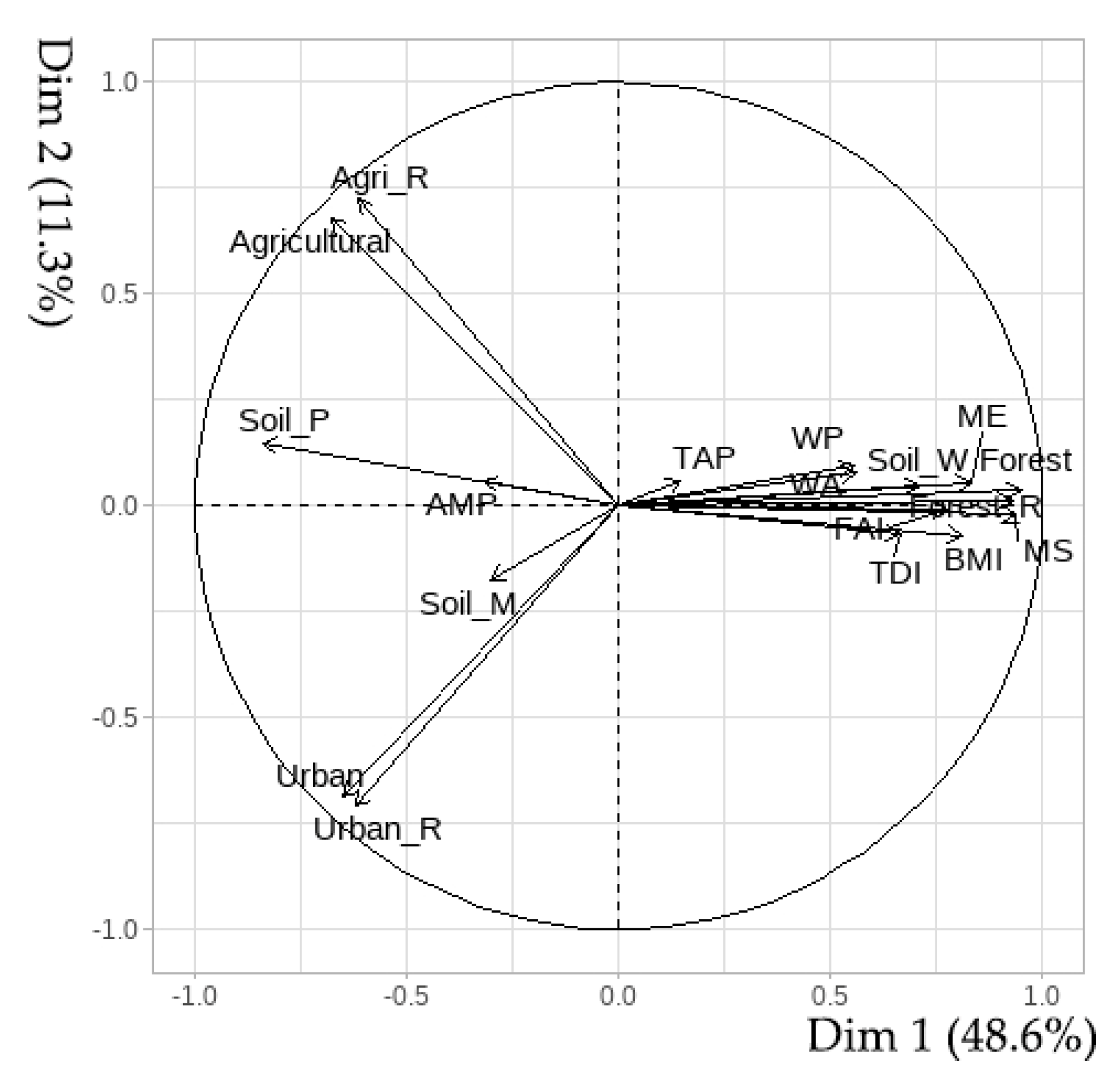
3.2. Principal Component Analysis

In our study, PCA was applied to simplify the watershed characteristics and biological condition of streams into PCs. Five PCs from the PCA analysis explained 84% of the total cumulative variance in the dataset with eigenvalues > 1 (Table 2). Table 3 presents the rotated factor loadings of the five PCs extracted from the PCA. Notably, PCs indicate the most meaningful variables with data reduction from the entire original dataset, while factor loading aids in understanding the basic characteristics of the PCs. As listed in Table 3, the first PC (PC1) accounts for 49% of the total variance in the dataset and has factor loadings on the mean slope, watershed forest area, and riparian forest area. The second PC (PC2), explaining 11% of the total variance, has positive loadings on agricultural areas at the watershed and riparian scale, and negative loadings on urban areas at both scales. This component represents land use variables that are anthropogenic pollution sources. Further, PC3, which explains 10% of the total variance, has factor loadings on the watershed area and perimeter, which are included in the watershed physiographic features. Next, PC4, explaining 8% of the total variance, has positive loadings on moderately drained soil and negative loadings on well-drained soil, which are both included as soil drainage variables. Finally, PC5 (6% of total variance) has factor loadings on the climate characteristics, including the total annual precipitation and annual maximum daily precipitation.
A PCA biplot, representing the loading vectors, was used to clarify the variables that are the most influential and how they are related to each other. Figure 2 shows a biplot of the first two PCs, which provides a general view on the variations in watershed characteristics and biological indicators. Their spatial locations indicate the similarity between them. Specifically, we assessed the relationships between the biological indicators of streams and watershed attributes based on the biplot. The plot indicates that the three biological indicators, TDI, BMI, and FAI, are positively correlated with mean slope, forest area, mean elevation, well-drained soil area, watershed area, watershed perimeter, and annual total annual precipitation, which are grouped together. In contrast, these three biological indicators are inversely correlated with moderately and poorly drained soil areas, annual maximum daily precipitation, agricultural land use, and urban land use, which are located on the opposite side of the biplot. In particular, the mean slope and forest area at the watershed and riparian scale have strong positive impacts on the biological indicators of streams, as indicated by the vectors that have a longer length and are more parallel to the PCs (i.e., PCA characteristics that reveal stronger impacts).

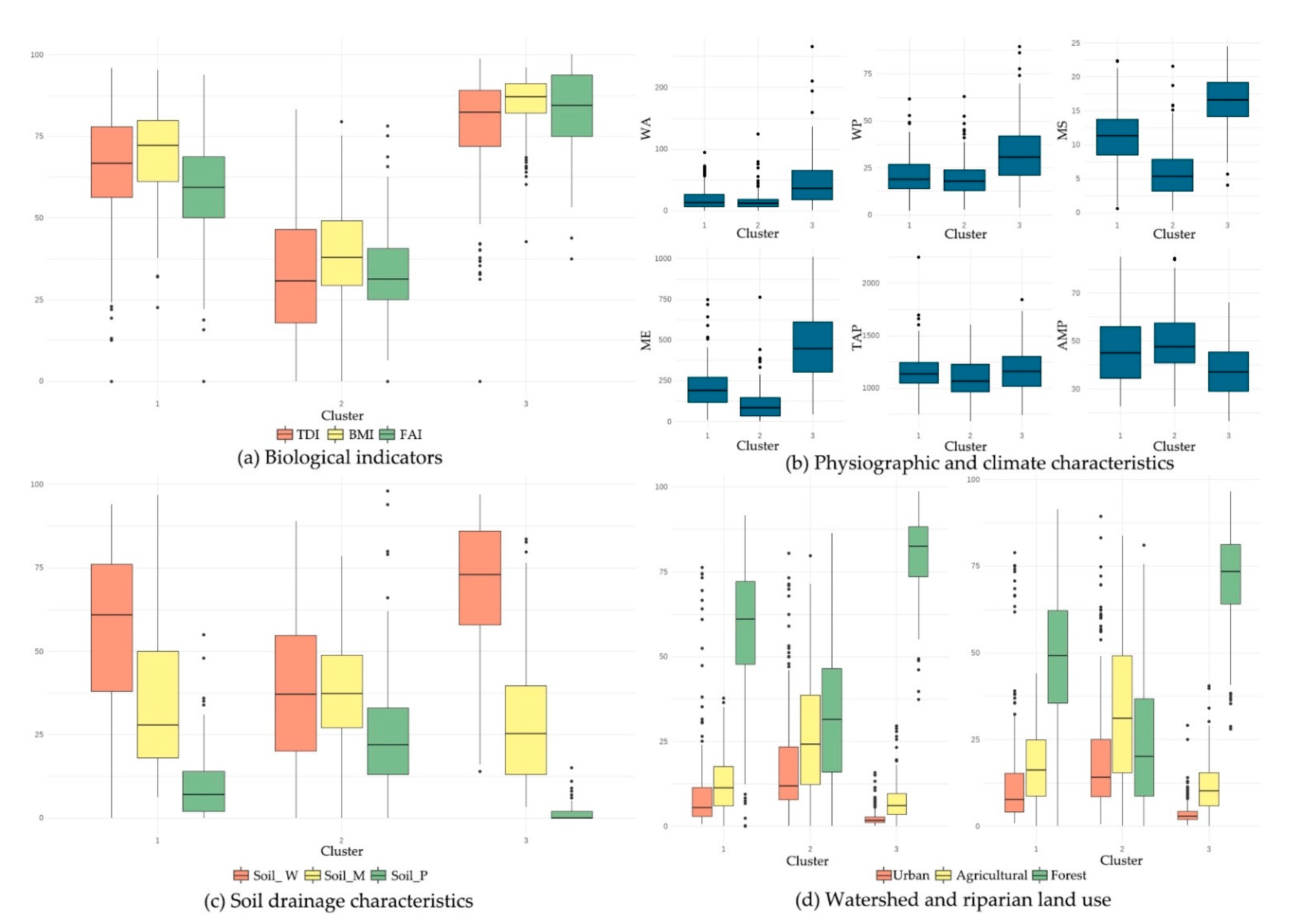
3.3. Self-Organizing Map Analysis

Figure 3 shows the trained SOM results for the watershed attributes and biological indicators of streams. Component planes of each variable with color gradients—from blue to red, representing the lowest and highest values, respectively—show the contribution of each variable. We interpreted the component planes by focusing on the relationships between the watershed attributes and biological indicators of streams. The biological indicators have similar patterns in their color gradients with watershed and riparian forest areas, mean slope, and well-drained soil. Their highest values occur in the middle area, whereas lower values appear at the top and bottom of the SOMs. Urban and agricultural areas at both scales and poorly drained soils show slightly similar distributions, with a pattern of several neurons at the top and bottom of the SOMs showing higher values than any other neurons, while the patterns for the biological indicators are the opposite. The component planes of the biological indicators have no notable common patterns with the watershed area, watershed perimeter, mean elevation, moderately drained soil, and climate characteristics. The SOM results indicate that the biological indicators have positive relationships with the mean slope, well-drained soil, and forest areas, whereas they have negative correlations with urban areas, agricultural areas, and poorly drained soil.3.4. Cluster Analysis
Watersheds were clustered into three groups with similar watershed attributes and biological conditions of streams based on the trained SOM units. Figure 4 and Figure 5 show the spatial distribution of the watersheds and radar plot for each cluster, respectively. Watersheds in cluster 1 are clustered in the central and western parts of the Han River Basin, where all watershed attributes and biological indicators have average values. The watersheds in cluster 2, representing a poor biological condition of streams, are almost completely dispersed in the western region, which is dominated by urban and agricultural lands with higher proportions of poorly drained soils (i.e., less forested land). The watersheds in cluster 3 show a good biological condition and are distributed in the eastern region, with greater values for watershed area, watershed perimeter, mean slope, mean elevation, well-drained soil, and forest areas.
Boxplots showing the median, interquartile range, and outliers of the variables within each cluster show notable differences among the groups (Figure 6). The values of the biological indicators are the highest in cluster 3 (good condition) and lowest in cluster 2 (poor condition). The physiographic attributes, including watershed area, watershed perimeter, mean slope, and mean elevation, have the highest values in cluster 3 and lowest values in cluster 2, while annual maximum daily precipitation is the lowest in cluster 3. Well-drained soil has the highest value in cluster 3 and lowest value in cluster 2. Forest areas at the watershed and riparian scale are the highest in cluster 3, while urban and agricultural areas at both scales are the highest in cluster 2.

4. Discussion

4.1. Relationship between Watershed Attributes and Biological Indicators

The results of our study indicate that the biological condition of a stream is positively related to forest areas, well-drained soil, and slope. Previous studies have shown that forests are closely associated with the transportation of pollutants and nutrients, surface runoff speed, and sediment discharge [49,50,51,52,53,54,55], which significantly affect water quality and aquatic ecosystems. Gu et al. [56] demonstrated that forests are the most important land use type that influences water quality. In terms of the slope and soil, undeveloped forested watersheds are generally located on steeper slopes, where there are no impervious areas, such as parking lots, roads, and buildings, resulting in low concentrations of pollutants, nutrients, and sediments, and a good biological condition of streams [57]. However, the effects of a slope on stream conditions may vary from region to region. Some studies have demonstrated that steeper slopes are associated with a decrease in pollutant concentrations [20,58], while others have shown that a higher slope increases the pollutant concentrations in downstream water bodies, which results in stream water quality degradation [59,60]. The results of our study also suggest that the biological condition of streams has a negative relationship with urban and agricultural areas. Many previous studies have reported that streams surrounded by urban and agricultural areas have poor water quality and aquatic ecosystems [61]. Urbanization increases the area of impervious surfaces, alters the watershed hydrology, and transports pollutants into waterbodies [62,63], while agricultural activities increase the nutrient concentrations in water bodies due to fertilizers and soil erosion [64]. The findings in our study highlight that land use planning and management strategies at the watershed and riparian scale are of critical importance for protecting and improving the biological condition of streams.
Furthermore, our findings indicate land use to have a greater effect on biological integrity of streams than the shape of a watershed and its climatic variables [27]. Clément et al. [18] investigated the effect of watershed characteristics (e.g., size, perimeter, land cover, and topographic variables) on stream water quality and biological conditions; they found that land cover and topography were more important than watershed size and perimeter for explaining the variations in stream water quality and biological conditions. We observed that streams with large catchment sizes had better biological conditions. It was more likely that larger watershed areas in this study had high proportions of forests. Thus, the large watershed areas are beneficial for preserving more forested areas within the watershed, resulting in better stream water quality and biological conditions. In addition, the biological conditions of streams can significantly vary due to differences in the topography of the watershed, as this affects the hydrological characteristics of a watershed and the transport of pollutants into streams [4]. If watershed and riparian land use are similar, higher slopes and elevations yield a higher probability that a pollutant will enter a water body, along with surface runoff [60]. However, if the proportions of land use are significantly different, land use can be a more influential factor on the biological condition of streams than topographic features, such as elevation and slope. For example, although cluster 3 has the highest elevation and slope compared with the other clusters, streams related to this cluster were in the best biological condition owing to the proportion of forest area being dominant.

4.2. Implications and Suggestions for Improving Watershed Planning and Management

Our findings provide a foundation for several important policies and management strategies for integrated watershed management. First, the results of our study highlight that land use planning and management should be considered a priority for protecting and restoring biological integrity of streams because land use is the most critical factor among several watershed attributes that determine the biological indicators of streams. Anthropogenic land use and land cover changes alter land surface features, such as elevation, slope, and soil, which affect hydrological processes in watersheds and cause aquatic ecosystem degradation [65]. As anthropogenic pressures can be managed, as opposed to natural factors, we emphasize the importance of local, regional, and national land use planning from a long-term perspective.
Second, similar to previous studies, our results reaffirm that acquiring forest cover in watershed and riparian buffers is of great significance for biological integrity of streams [56,66]. Although conserving existing forests and increasing the proportion of forest cover is the ideal method to improve the biological health of streams, maintaining the proportion of forest areas is difficult owing to developmental pressure from urban areas. Therefore, for responsible land use development, urban planning and the development process should consider provisions of GI, as well as increasing the connectivity of GI, as an alternative to forest areas, including bioswales, rain gardens, green roofs, and permeable pavement. Furthermore, at the national level, the Korean government is planning to enforce the “no net loss” policy for natural resources such as forests and wetlands. This policy states that the total amount of natural resources should be conserved by restoring the quantity of natural resources damaged by construction activities to offset the impacts of development. Development should be strictly prohibited in riparian areas adjacent to streams. Any existing built-up and cultivated land in these areas should be gradually relocated, and the original area restored into vegetated area. Moreover, stream restoration should be undertaken at the riparian scale, as riparian vegetation has various functions, such as mitigating the anthropogenic impacts of watershed land use on streams.
Third, characterizing watersheds into meaningful groups can assist in detecting the features of regional biological conditions, and establish priorities by adopting different strategies based on watershed similarities. In the Han River Basin, most watersheds with streams in a poor biological condition are distributed in the western region, where urban and agricultural areas are dominant. In contrast, watersheds with streams in a good biological condition are dispersed in the eastern region, where forest areas are dominant. Management strategies in cluster 3 watersheds (good biological condition) should focus on protection; however, in cluster 2, characterized by a high proportion of urban and agricultural areas, strategies should be approached from the perspective of restoration. In particular, the watersheds and streams in cluster 3 can be a reference for restoring damaged watersheds and streams. However, even if watershed characteristics are similar, hydrological processes and watershed responses can be spatially different. Therefore, there is still a need for analyzing and comprehensively understanding watershed systems at smaller scales [67].

5. Conclusions

In this study, we identified key watershed characteristics that affect stream ecosystems across the Han River watershed in South Korea using PCA and SOM. Our findings indicate that land use can have a larger effect on biological indicators than the topography of a watershed and its climatic variables. The examined watersheds were classified into three clusters, representing clear differences in land use variables and biological indicators between clusters. The group with streams in a good biological condition was distributed in the eastern region, with a high proportion of forest areas, while the group with streams in a poor biological condition was dispersed in the western region, with a high proportion of urban and agricultural areas. The findings of this study emphasize that land use planning and management at the watershed and riparian scale, particularly related to an increase in the amount of forest areas, are critically important for protecting and improving the biological condition of streams. Our results also provide a foundation for managers and policymakers to establish priorities by adopting different strategies based on similar watershed characteristics. In the studied area, management strategies in cluster 3 watersheds should focus on protection, whereas, in cluster 2, strategies should be approached from the perspective of restoration. However, further studies should be carried out to classify watersheds into various regions with other variables.

Author Contributions

S.-R.P. was responsible for the study conception, collecting data, and writing the original draft; S.-J.H. contributed to the interpretation of the statistics and edited the manuscript; K.A. interpreted the results of the analysis and edited the manuscript; S.-W.L. performed statistical analyses and edited the manuscript. All authors have read and agreed to the published version of the manuscript.

Funding

This work was supported by the Korea Environment Industry and Technology Institute (KEITI) through The Decision Support System Development Project for Environmental Impact Assessment, funded by the Korea Ministry of Environment (MOE) (No. 2020002990009). This study was also supported by a National Research Foundation of Korea (NRF) grant funded by the Korean government (MSIT) (No. 2019R1F1A1063823).

Institutional Review Board Statement

Not applicable.

Informed Consent Statement

Not applicable.

Data Availability Statement

No new data were created and analyzed in this study. Data sharing is not applicable to this article.

Conflicts of Interest

The authors declare no conflict of interest.

References

  1. United States Environmental Protection Agency. Available online: https://www.epa.gov/ (accessed on 23 February 2021).
  2. Hou, Y.; Li, B.; Müller, F.; Chen, W. Ecosystem Services of Human-Dominated Watersheds and Land use Influences: A Case Study from the Dianchi Lake Watershed in China. Environ. Monit. Assess. 2016, 188, 1–19. [Google Scholar] [CrossRef] [Green Version]
  3. Baker, A. Land use and Water Quality. In Encyclopedia of Hydrological Sciences; John Wiley & Sons, Ltd.: Chichester, UK, 2006; Volume 17. [Google Scholar] [CrossRef]
  4. Price, K. Effects of Watershed Topography, Soils, Land use, and Climate on Baseflow Hydrology in Humid Regions: A Review. Prog. Phys. Geogr. 2011, 35, 465–492. [Google Scholar] [CrossRef]
  5. Miserendino, M.L.; Casaux, R.; Archangelsky, M.; Di Prinzio, C.Y.; Brand, C.; Kutschker, A.M. Assessing Land-use Effects on Water Quality, in-Stream Habitat, Riparian Ecosystems and Biodiversity in Patagonian Northwest Streams. Sci. Total Environ. 2011, 409, 612–624. [Google Scholar] [CrossRef] [PubMed]
  6. Ficklin, D.L.; Stewart, I.T.; Maurer, E.P. Effects of Climate Change on Stream Temperature, Dissolved Oxygen, and Sediment Concentration in the Sierra Nevada in California. Water Resour. Res. 2013, 49, 2765–2782. [Google Scholar] [CrossRef]
  7. Mosley, L.M. Drought Impacts on the Water Quality of Freshwater Systems; Review and Integration. Earth Sci. Rev. 2015, 140, 203–214. [Google Scholar] [CrossRef]
  8. Chang, H.; Bonnette, M.R.; Stoker, P.; Crow-Miller, B.; Wentz, E. Determinants of Single Family Residential Water use Across Scales in Four Western US Cities. Sci. Total Environ. 2017, 596, 451–464. [Google Scholar] [CrossRef]
  9. Park, Y.; Lee, S.; Lee, J. Comparison of Fuzzy AHP and AHP in Multicriteria Inventory Classification while Planning Green Infrastructure for Resilient Stream Ecosystems. Sustainability 2020, 12, 9035. [Google Scholar] [CrossRef]
  10. Young, R.F. Planting the Living City: Best Practices in Planning Green infrastructure—Results from Major Us Cities. J. Am. Plan. Assoc. 2011, 77, 368–381. [Google Scholar] [CrossRef]
  11. Ellis, J.B. Sustainable Surface Water Management and Green Infrastructure in UK Urban Catchment Planning. J. Environ. Plan. Manag. 2013, 56, 24–41. [Google Scholar] [CrossRef]
  12. Liu, L.; Jensen, M.B. Green Infrastructure for Sustainable Urban Water Management: Practices of Five Forerunner Cities. Cities 2018, 74, 126–133. [Google Scholar] [CrossRef]
  13. McFarland, A.R.; Larsen, L.; Yeshitela, K.; Engida, A.N.; Love, N.G. Guide for using Green Infrastructure in Urban Environments for Stormwater Management. Environ. Sci. Water Res. Technol. 2019, 5, 643–659. [Google Scholar] [CrossRef]
  14. Keeley, M.; Koburger, A.; Dolowitz, D.P.; Medearis, D.; Nickel, D.; Shuster, W. Perspectives on the use of Green Infrastructure for Stormwater Management in Cleveland and Milwaukee. Environ. Manag. 2013, 51, 1093–1108. [Google Scholar] [CrossRef]
  15. Lee, S.; Hwang, S.; Lee, S.; Hwang, H.; Sung, H. Landscape Ecological Approach to the Relationships of Land use Patterns in Watersheds to Water Quality Characteristics. Landsc. Urban Plann. 2009, 92, 80–89. [Google Scholar] [CrossRef]
  16. Carey, R.O.; Migliaccio, K.W.; Li, Y.; Schaffer, B.; Kiker, G.A.; Brown, M.T. Land use Disturbance Indicators and Water Quality Variability in the Biscayne Bay Watershed, Florida. Ecol. Ind. 2011, 11, 1093–1104. [Google Scholar] [CrossRef]
  17. Álvarez-Cabria, M.; Barquín, J.; Peñas, F.J. Modelling the Spatial and Seasonal Variability of Water Quality for Entire River Networks: Relationships with Natural and Anthropogenic Factors. Sci. Total Environ. 2016, 545, 152–162. [Google Scholar] [CrossRef]
  18. Clément, F.; Ruiz, J.; Rodríguez, M.A.; Blais, D.; Campeau, S. Landscape Diversity and Forest Edge Density Regulate Stream Water Quality in Agricultural Catchments. Ecol. Ind. 2017, 72, 627–639. [Google Scholar] [CrossRef]
  19. Giri, S.; Zhang, Z.; Krasnuk, D.; Lathrop, R.G. Evaluating the Impact of Land Uses on Stream Integrity using Machine Learning Algorithms. Sci. Total Environ. 2019, 696, 133858. [Google Scholar] [CrossRef]
  20. Chen, J.; Lu, J. Effects of Land use, Topography and Socio-Economic Factors on River Water Quality in a Mountainous Watershed with Intensive Agricultural Production in East China. PLoS ONE 2014, 9, e102714. [Google Scholar] [CrossRef] [PubMed]
  21. Varanka, S.; Hjort, J.; Luoto, M. Geomorphological Factors Predict Water Quality in Boreal Rivers. Earth Surf. Process. Landf. 2015, 40, 1989–1999. [Google Scholar] [CrossRef]
  22. Alnahit, A.O.; Mishra, A.K.; Khan, A.A. Quantifying Climate, Streamflow, and Watershed Control on Water Quality across Southeastern US Watersheds. Sci. Total Environ. 2020, 739, 139945. [Google Scholar] [CrossRef] [PubMed]
  23. Wang, L.; Lyons, J.; Kanehl, P.; Gatti, R. Influences of Watershed Land use on Habitat Quality and Biotic Integrity in Wisconsin Streams. Fisheries 1997, 22, 6–12. [Google Scholar] [CrossRef]
  24. Waite, I.R.; Brown, L.R.; Kennen, J.G.; May, J.T.; Cuffney, T.F.; Orlando, J.L.; Jones, K.A. Comparison of Watershed Disturbance Predictive Models for Stream Benthic Macroinvertebrates for Three Distinct Ecoregions in Western US. Ecol. Ind. 2010, 10, 1125–1136. [Google Scholar] [CrossRef]
  25. Hwang, S.; Hwang, S.; Park, S.; Lee, S. Examining the Relationships between Watershed Urban Land use and Stream Water Quality using Linear and Generalized Additive Models. Water 2016, 8, 155. [Google Scholar] [CrossRef] [Green Version]
  26. Mayer, A.; Winkler, R.; Fry, L. Classification of Watersheds into Integrated Social and Biophysical Indicators with Clustering Analysis. Ecol. Ind. 2014, 45, 340–349. [Google Scholar] [CrossRef]
  27. Park, Y.; Kwon, Y.; Hwang, S.; Park, S. Characterizing Effects of Landscape and Morphometric Factors on Water Quality of Reservoirs using a Self-Organizing Map. Environ. Model. Softw. 2014, 55, 214–221. [Google Scholar] [CrossRef]
  28. Singh, K.P.; Malik, A.; Mohan, D.; Sinha, S. Multivariate Statistical Techniques for the Evaluation of Spatial and Temporal Variations in Water Quality of Gomti River (India)—A Case Study. Water Res. 2004, 38, 3980–3992. [Google Scholar] [CrossRef] [PubMed]
  29. Tran, C.P.; Bode, R.W.; Smith, A.J.; Kleppel, G.S. Land-use Proximity as a Basis for Assessing Stream Water Quality in New York State (USA). Ecol. Indic. 2010, 10, 727–733. [Google Scholar] [CrossRef]
  30. Barakat, A.; El Baghdadi, M.; Rais, J.; Aghezzaf, B.; Slassi, M. Assessment of Spatial and Seasonal Water Quality Variation of Oum Er Rbia River (Morocco) using Multivariate Statistical Techniques. Int. Soil Water Conserv. Res. 2016, 4, 284–292. [Google Scholar] [CrossRef]
  31. Razavi, T.; Coulibaly, P. Classification of Ontario Watersheds Based on Physical Attributes and Streamflow Series. J. Hydrol. 2013, 493, 81–94. [Google Scholar] [CrossRef]
  32. Li, T.; Sun, G.; Yang, C.; Liang, K.; Ma, S.; Huang, L. Using Self-Organizing Map for Coastal Water Quality Classification: Towards a Better Understanding of Patterns and Processes. Sci. Total Environ. 2018, 628, 1446–1459. [Google Scholar] [CrossRef]
  33. Ley, R.; Casper, M.C.; Hellebrand, H.; Merz, R. Catchment Classification by Runoff Behaviour with Self-Organizing Maps (SOM). Hydrol. Earth Syst. Sci. 2011, 15, 2947–2962. [Google Scholar] [CrossRef] [Green Version]
  34. Jung, K.Y.; Lee, K.; Im, T.H.; Lee, I.J.; Kim, S.; Han, K.; Ahn, J.M. Evaluation of Water Quality for the Nakdong River Watershed using Multivariate Analysis. Environ. Technol. Innov. 2016, 5, 67–82. [Google Scholar] [CrossRef]
  35. Ministry of Environment (MOE). National Water Environment Management Plan for Han River Basin; Korean Literature; Han River Basin Environmental Office: Gyeonggi-do, Korea, 2015.
  36. Wang, G.; Mang, S.; Cai, H.; Liu, S.; Zhang, Z.; Wang, L.; Innes, J.L. Integrated Watershed Management: Evolution, Development and Emerging Trends. J. For. Res. 2016, 27, 967–994. [Google Scholar] [CrossRef] [Green Version]
  37. Gurung, B.; Race, M.; Fabbricino, M.; Komínková, D.; Libralato, G.; Siciliano, A.; Guida, M. Assessment of Metal Pollution in the Lambro Creek (Italy). Ecotoxicol. Environ. Saf. 2018, 148, 754–762. [Google Scholar] [CrossRef]
  38. Kelly, M.G.; Whitton, B.A. The Trophic Diatom Index: A New Index for Monitoring Eutrophication in Rivers. J. Appl. Phycol. 1995, 7, 433–444. [Google Scholar] [CrossRef]
  39. Karr, J.R. Defining and Measuring River Health. Freshw. Biol. 1999, 41, 221–234. [Google Scholar] [CrossRef] [Green Version]
  40. Lee, S.; Hwang, S.; Lee, J.; Jung, D.; Park, Y.; Kim, J. Overview and Application of the National Aquatic Ecological Monitoring Program (NAEMP) in Korea. Ann. Limnol. Int. J. Limnol. 2011, 47, S3–S14. [Google Scholar] [CrossRef]
  41. Erba, S.; Pace, G.; Demartini, D.; Di Pasquale, D.; Dörflinger, G.; Buffagni, A. Land use at the Reach Scale as a Major Determinant for Benthic Invertebrate Community in Mediterranean Rivers of Cyprus. Ecol. Ind. 2015, 48, 477–491. [Google Scholar] [CrossRef]
  42. Jonsson, M.; Burrows, R.M.; Lidman, J.; Fältström, E.; Laudon, H.; Sponseller, R.A. Land use Influences Macroinvertebrate Community Composition in Boreal Headwaters through Altered Stream Conditions. Ambio 2017, 46, 311–323. [Google Scholar] [CrossRef] [Green Version]
  43. Ministry of Environment and National Institute of Environmental Research (MOE and NIER). Waterwide Aquatic Ecological Monitoring Program (V); Korean Literature; Korean Literature; Ministry of Environment and National Institute of Environmental Research: Incheon, Korea, 2012.
  44. Abdi, H.; Williams, L.J. Principal Component Analysis. Wiley Interdiscip. Rev. Comput. Stat. 2010, 2, 433–459. [Google Scholar] [CrossRef]
  45. Kalteh, A.M.; Hjorth, P.; Berndtsson, R. Review of the Self-Organizing Map (SOM) Approach in Water Resources: Analysis, Modelling and Application. Environ. Model. Softw. 2008, 23, 835–845. [Google Scholar] [CrossRef]
  46. Baghanam, A.H.; Nourani, V.; Aslani, H.; Taghipour, H. Spatiotemporal Variation of Water Pollution Near Landfill Site: Application of Clustering Methods to Assess the Admissibility of LWPI. J. Hydrol. 2020, 591, 125581. [Google Scholar] [CrossRef]
  47. Clark, S.; Sisson, S.A.; Sharma, A. Tools for Enhancing the Application of Self-Organizing Maps in Water Resources Research and Engineering. Adv. Water Resour. 2020, 103676. [Google Scholar] [CrossRef]
  48. Kohonen, T. Self-Organizing Maps; Springer Science & Business Media: Berlin, Germany, 2012. [Google Scholar]
  49. Tabacchi, E.; Lambs, L.; Guilloy, H.; Planty-Tabacchi, A.; Muller, E.; Decamps, H. Impacts of Riparian Vegetation on Hydrological Processes. Hydrol. Process. 2000, 14, 2959–2976. [Google Scholar] [CrossRef]
  50. Broadmeadow, S.; Nisbet, T.R. The Effects of Riparian Forest Management on the Freshwater Environment: A Literature Review of Best Management Practice. Hydrol. Earth Syst. Sci. 2004, 8, 286–305. [Google Scholar] [CrossRef]
  51. Carlisle, D.M.; Falcone, J.; Meador, M.R. Predicting the Biological Condition of Streams: Use of Geospatial Indicators of Natural and Anthropogenic Characteristics of Watersheds. Environ. Monit. Assess. 2009, 151, 143–160. [Google Scholar] [CrossRef]
  52. Taniwaki, R.H.; Cassiano, C.C.; Filoso, S.; de Barros Ferraz, S.F.; de Camargo, P.B.; Martinelli, L.A. Impacts of Converting Low-Intensity Pastureland to High-Intensity Bioenergy Cropland on the Water Quality of Tropical Streams in Brazil. Sci. Total Environ. 2017, 584, 339–347. [Google Scholar] [CrossRef] [PubMed]
  53. Li, K.; Chi, G.; Wang, L.; Xie, Y.; Wang, X.; Fan, Z. Identifying the Critical Riparian Buffer Zone with the Strongest Linkage between Landscape Characteristics and Surface Water Quality. Ecol. Ind. 2018, 93, 741–752. [Google Scholar] [CrossRef]
  54. Yirigui, Y.; Lee, S.; Nejadhashemi, A.P. Multi-Scale Assessment of Relationships between Fragmentation of Riparian Forests and Biological Conditions in Streams. Sustainability 2019, 11, 5060. [Google Scholar] [CrossRef] [Green Version]
  55. Yirigui, Y.; Lee, S.; Nejadhashemi, A.P.; Herman, M.R.; Lee, J. Relationships between Riparian Forest Fragmentation and Biological Indicators of Streams. Sustainability 2019, 11, 2870. [Google Scholar] [CrossRef] [Green Version]
  56. Gu, H.; Wang, J.; Ma, L.; Shang, Z.; Zhang, Q. Insights into the BRT (Boosted Regression Trees) Method in the Study of the Climate-Growth Relationship of Masson Pine in Subtropical China. Forests 2019, 10, 228. [Google Scholar] [CrossRef] [Green Version]
  57. Yu, S.; Xu, Z.; Wu, W.; Zuo, D. Effect of Land use Types on Stream Water Quality Under Seasonal Variation and Topographic Characteristics in the Wei River Basin, China. Ecol. Indic. 2016, 60, 202–212. [Google Scholar] [CrossRef]
  58. Chang, H. Spatial Analysis of Water Quality Trends in the Han River Basin, South Korea. Water Res. 2008, 42, 3285–3304. [Google Scholar] [CrossRef]
  59. Sliva, L.; Williams, D.D. Buffer Zone Versus Whole Catchment Approaches to Studying Land use Impact on River Water Quality. Water Res. 2001, 35, 3462–3472. [Google Scholar] [CrossRef]
  60. Ye, L.; Cai, Q.; Liu, R.; Cao, M. The Influence of Topography and Land use on Water Quality of Xiangxi River in Three Gorges Reservoir Region. Environ. Geol. 2009, 58, 937–942. [Google Scholar] [CrossRef]
  61. Liu, J.; Shen, Z.; Chen, L. Assessing how Spatial Variations of Land use Pattern Affect Water Quality Across a Typical Urbanized Watershed in Beijing, China. Landsc. Urban Plan. 2018, 176, 51–63. [Google Scholar] [CrossRef]
  62. Wilson, C.; Weng, Q. Assessing Surface Water Quality and its Relation with Urban Land Cover Changes in the Lake Calumet Area, Greater Chicago. Environ. Manag. 2010, 45, 1096–1111. [Google Scholar] [CrossRef] [PubMed]
  63. Kennen, J.G.; Riva-Murray, K.; Beaulieu, K.M. Determining Hydrologic Factors that Influence Stream Macroinvertebrate Assemblages in the Northeastern US. Ecohydrol. Ecosyst. Land Water Process Interact. Ecohydrogeomorphol. 2010, 3, 88–106. [Google Scholar] [CrossRef]
  64. Zhou, T.; Wu, J.; Peng, S. Assessing the Effects of Landscape Pattern on River Water Quality at Multiple Scales: A Case Study of the Dongjiang River Watershed, China. Ecol. Ind. 2012, 23, 166–175. [Google Scholar] [CrossRef]
  65. Dwarakish, G.S.; Ganasri, B.P. Impact of Land use Change on Hydrological Systems: A Review of Current Modeling Approaches. Cogent Geosci. 2015, 1, 1115691. [Google Scholar] [CrossRef]
  66. Ding, S.; Zhang, Y.; Liu, B.; Kong, W.; Meng, W. Effects of Riparian Land use on Water Quality and Fish Communities in the Headwater Stream of the Taizi River in China. Front. Environ. Sci. Eng. 2013, 7, 699–708. [Google Scholar] [CrossRef]
  67. Singh, S.K.; McMillan, H.; Bárdossy, A.; Fateh, C. Nonparametric Catchment Clustering using the Data Depth Function. Hydrol. Sci. J. 2016, 61, 2649–2667. [Google Scholar] [CrossRef]
Figure 1. Han national watershed management regions (NWMR), topography (see color bar), and monitoring sites (red circles in enlarged image) of the National Aquatic Ecological Monitoring Program in Korea. Streams and lakes are shown in blue.
Sustainability 13 03359 g001
Figure 2. Principal component analysis (PCA) biplot for the first two principal component (PC) scores. TDI = trophic diatom index; BMI = benthic macroinvertebrate index; FAI = fish assessment index; WA = watershed area; WP = watershed perimeter; MS = mean slope; ME = mean elevation; Urban_R, Agri_R, and Forest_R = proportion of urban, agricultural, and forest land use at the riparian scale, respectively; Soil_W = well-drained soil; Soil_M = moderately drained soil; Soil_P = poorly drained soil; TAP = total annual precipitation; and AMP = annual maximum daily precipitation.
Sustainability 13 03359 g002
Figure 3. Component planes for the variables in the self-organizing map (SOM) results. Warm colors (reds) indicate high values, while cold colors (blues) represent low values. TDI = trophic diatom index; BMI = benthic macroinvertebrate index; FAI = fish assessment index; WA = watershed area (km2); WP = watershed perimeter (km); MS = mean slope (%); ME = mean elevation (m); Urban_R, Agri_R, and Forest_R = proportion of urban, agricultural, and forest land use at the riparian scale, respectively; Soil_W = well-drained soil (%); Soil_M = moderately drained soil (%); Soil_P = poorly drained soil (%); TAP = total annual precipitation (mm); and AMP = annual maximum daily precipitation (mm).
Sustainability 13 03359 g003
Figure 4. Spatial distribution of the three clustered groups, cluster 1 (yellow), 2 (red), and 3 (green), based on the self-organizing map (SOM) results. Unmonitored watersheds are denoted by a gray color.
Sustainability 13 03359 g004
Figure 5. Radar plot for the three clusters, cluster 1 (yellow), 2 (red), and 3 (green), with watershed attributes and biological indicators. TDI = trophic diatom index; BMI = benthic macroinvertebrate index; FAI = fish assessment index; WA = watershed area; WP = watershed perimeter; MS = mean slope; ME = mean elevation; Urban_R, Agri_R, and Forest_R = proportion of urban, agricultural, and forest land use at the riparian scale, respectively; Soil_W = well-drained soil; Soil_M = moderately drained soil; Soil_P = poorly drained soil; TAP = total annual precipitation; and AMP = annual maximum daily precipitation.
Sustainability 13 03359 g005
Figure 6. Boxplots of watershed attributes and biological indicators of streams for each group. (a) Biological indicators (TDI: trophic diatom index; BMI: benthic macroinvertebrate index; and FAI: fish assessment index); (b) physiographic and climate characteristics (WA: watershed area; WP: watershed perimeter; MS: mean slope; ME: mean elevation; TAP: total annual precipitation; and AMP: annual maximum daily precipitation); (c) soil drainage characteristics; and (d) watershed (left) and riparian (right) land use.
Sustainability 13 03359 g006
Table 1. Descriptive statistics of the watershed attributes and biological indicators of streams in the Han River Basin.
ClassificationVariablesMeanS.D.Min.Max.
Biological
indicators
TDI (0–100)61.525.10.098.7
BMI (0–100)67.422.10.096.1
FAI (0–100)60.724.70.0100.0
Physiographic
features
Watershed area (km2)29.233.10.3266.2
Watershed perimeter (km)25.414.32.389.4
Mean slope (%)11.75.70.324.5
Mean elevation (m)277.4218.41.81008.6
Watershed land useUrban area (%)9.613.50.080.5
Agricultural area (%)14.513.80.079.8
Forest area (%)59.225.50.098.6
Riparian land useUrban area (%)11.514.50.289.4
Agricultural area (%)19.215.90.083.7
Forest area (%)50.425.70.096.5
Soil drainageWell-drained (%)56.324.70.097.0
Moderately drained (%)33.219.10.096.7
Poorly drained (%)10.614.10.098.0
Climate
characteristics
Total annual precipitation (mm)1145.7188.8684.02248.0
Annual daily maximum precipitation (mm)44.113.516.585.0
n = 754. S.D. = Standard Deviation, Min. = Minimum, Max. = Maximum, TDI = Trophic Diatom Index, BMI = Benthic Macroinvertebrate Index, and FAI = Fish Assessment Index.
Table 2. Initial eigenvalues and variance for the principal components (PCs).
VariablePC 1PC 2PC 3PC 4PC 5PC 6PC 7PC 8PC 9
Eigenvalues2.961.431.351.191.000.900.750.650.57
Proportion of variance0.490.110.100.080.060.040.030.020.02
Cumulative proportion0.490.600.700.780.840.880.910.940.95
Table 3. Rotated factor matrix extracted from the principal component analysis (PCA).
VariableComponent
12345
TDI–0.23–0.05–0.01–0.01–0.16
BMI–0.27–0.05–0.050.09–0.19
FAI–0.26–0.010.030.12–0.19
WA–0.190.060.52–0.010.39
WP–0.190.070.510.010.39
MS–0.32–0.01–0.020.040.03
ME–0.280.040.160.070.06
Urban0.22–0.480.10–0.100.10
Agricultural0.230.470.070.00–0.06
Forest–0.320.03–0.070.060.01
Urban_R0.21–0.500.11–0.100.11
Agri_R0.210.510.10–0.01–0.03
Forest_R–0.310.01–0.100.06–0.02
Well-drained soil–0.240.03–0.22–0.500.12
Moderately drained soil0.10–0.120.180.72–0.20
Poorly drained soil0.280.100.13–0.100.06
TAP–0.050.04–0.400.350.43
AMP0.110.04–0.360.200.57
TDI = trophic diatom index; BMI = benthic macroinvertebrate index; FAI = fish assessment index; WA = watershed area; WP = watershed perimeter; MS = mean slope; ME = mean elevation; Urban_R, Agri_R, and Forest_R = proportion of urban, agricultural, and forest land use at the riparian scale, respectively; TAP = total annual precipitation; and AMP = annual maximum daily precipitation. Bold font indicates strong factor loading on each component.
Publisher’s Note: MDPI stays neutral with regard to jurisdictional claims in published maps and institutional affiliations.

