
Analyzing the Spatial Heterogeneity of the Built Environment and Its Impact on the Urban Thermal Environment—Case Study of Downtown Shanghai


Abstract
:1. Introduction
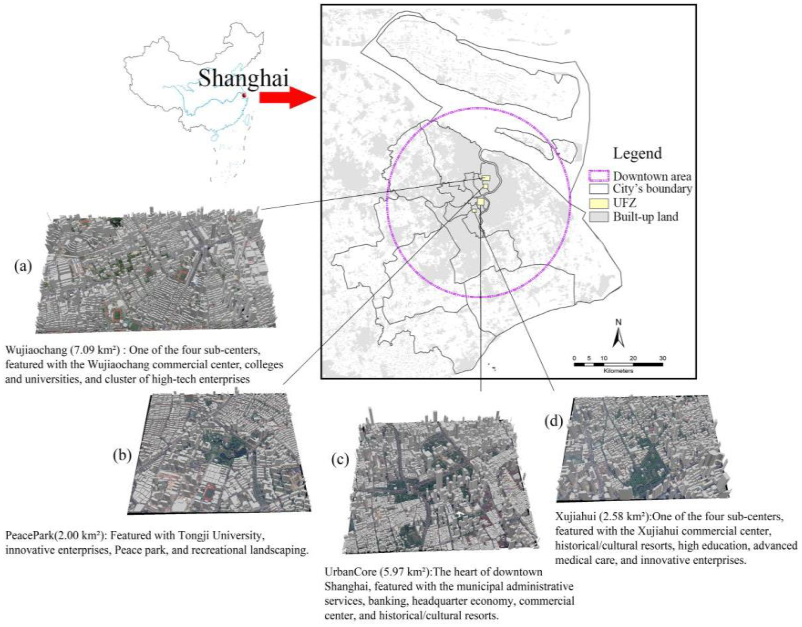
2. Study Area
3. Materials and Methods
3.1. Materials
3.2. Methods
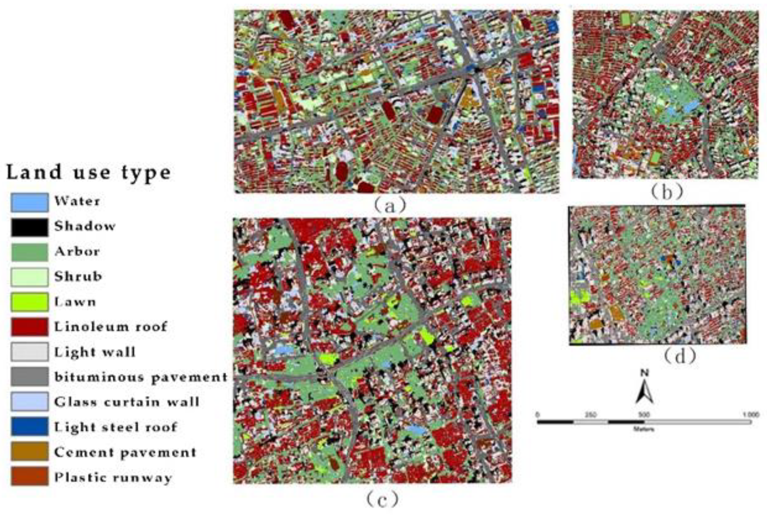
3.2.1. Land-Use Classification
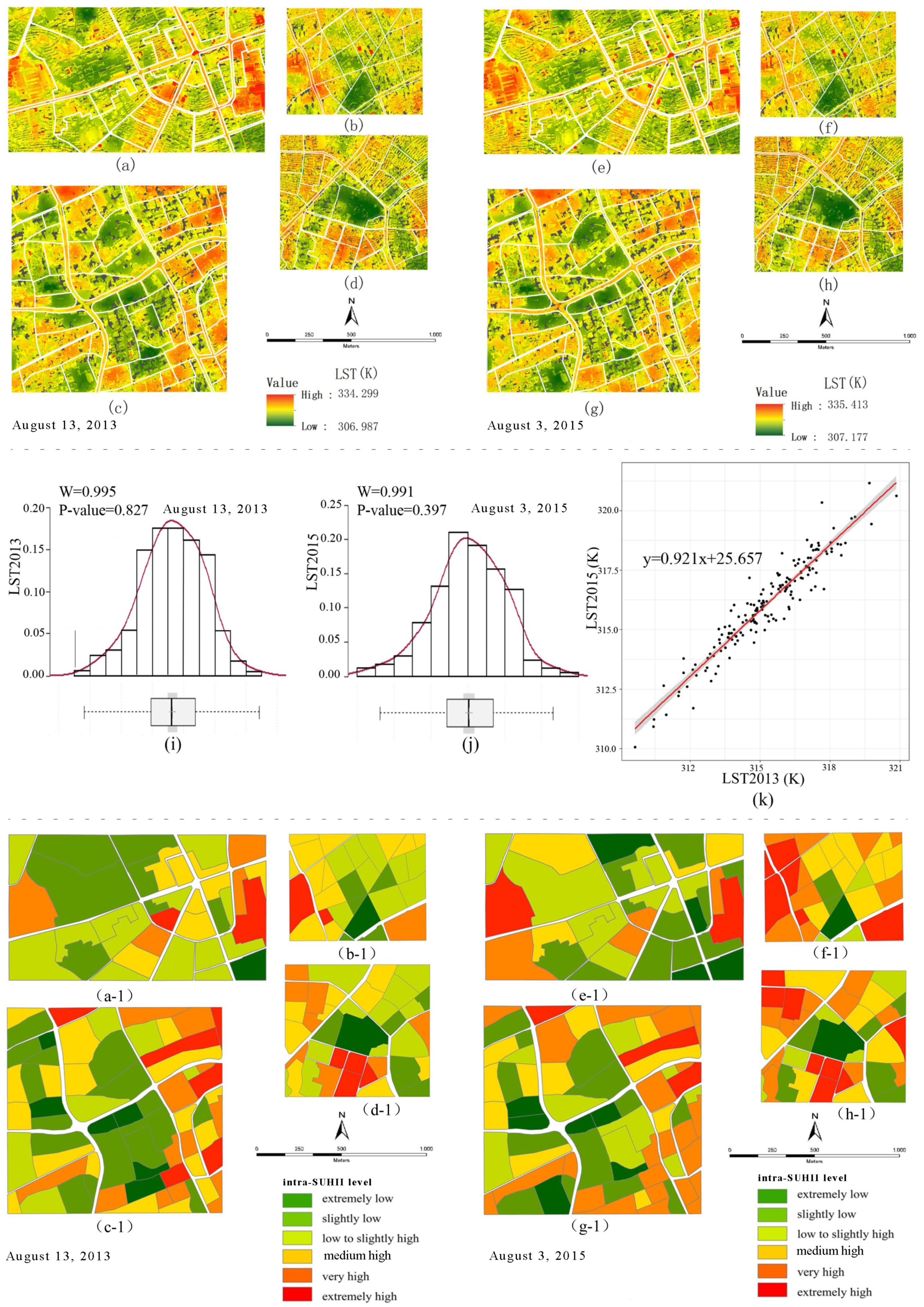
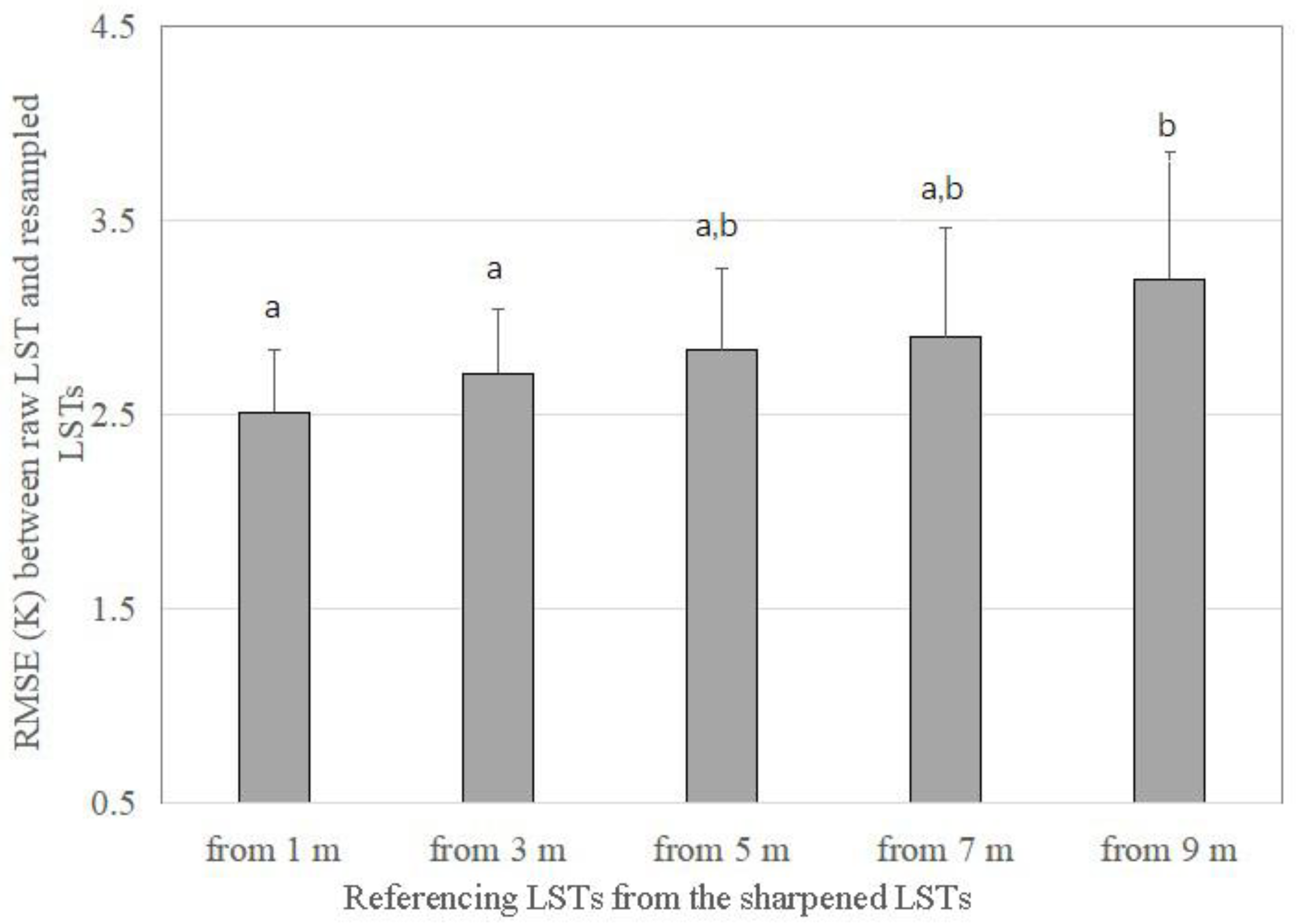
3.2.2. Generation of Thermally Sharpened LST and Cross-Validation
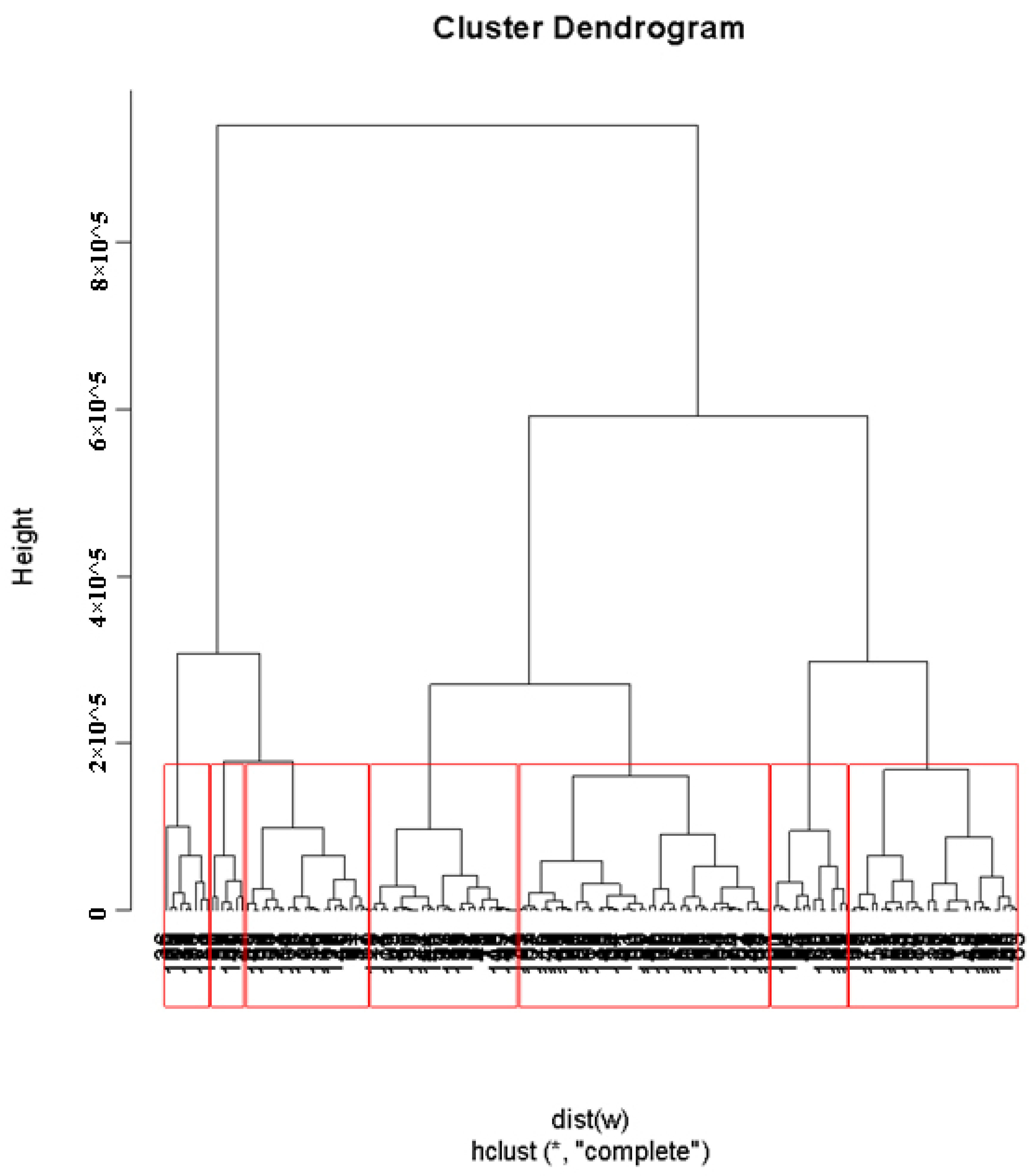
3.2.3. Calculation of Intra-SUHII
3.2.4. Statistical Analysis
4. Results
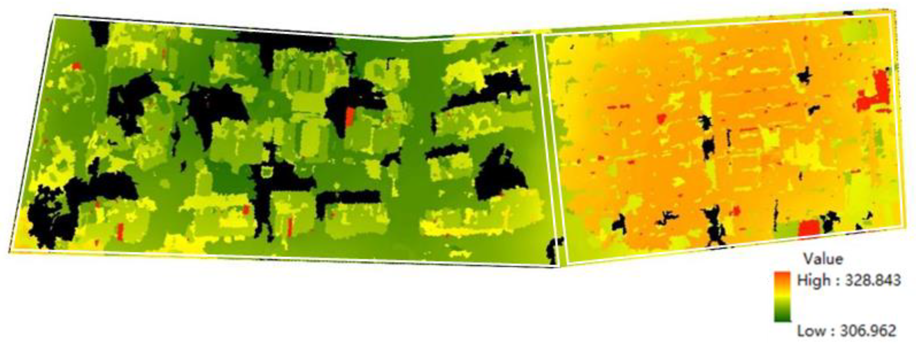
4.1. Spatial Distribution Characteristics of the Urban Thermal Environment
4.2. Relationship between the Spatial Heterogeneity of the Built Environment and the Urban Thermal Environment
5. Discussion
6. Conclusions
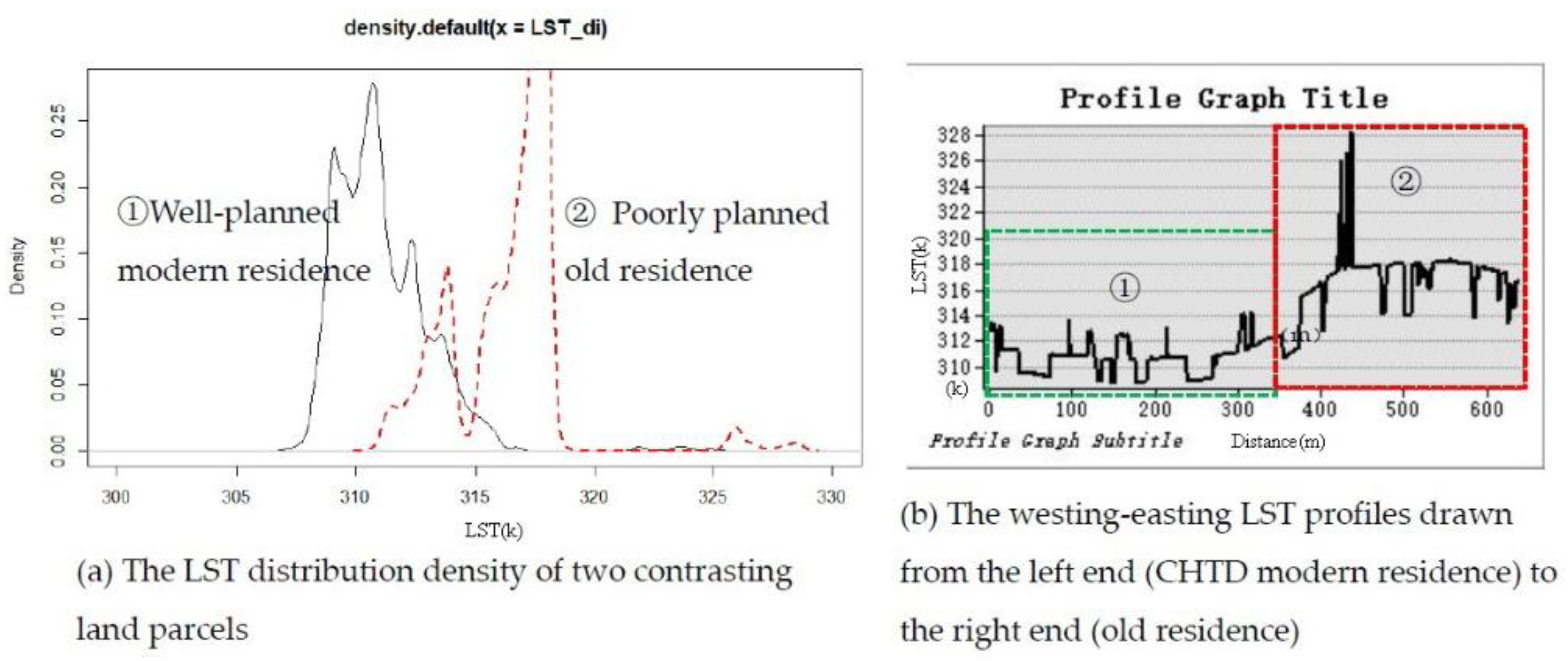
- There are remarkable variations of LSTs and intra-SUHII among seven typical land parcels with different land developmental intensities. Overall, land parcels featured with dominant BGS and lower impervious surfaces, particularly parks and recreational landscapes, a university/college campus with a higher green cover, and well-planned modern residences exhibited much lower mean LSTs than the other land parcel types with dense buildings and lacking BGS.
- The PLSR models quantitatively revealed the relative importance of the main effect of the urban built environment in determining the variances of the urban thermal environment. The results show that the building distance/spacing, SVF, LPI, and BGS are major negative contributors to decreasing the variance of the parcel-based intra-SUHI effect. In contrast, the ImperSurf and SPLIT are major positive contributors to increasing the variance of the parcel-based intra-SUHI effect.
Author Contributions
Funding
Institutional Review Board Statement
Informed Consent Statement
Data Availability Statement
Conflicts of Interest
Appendix A

| Categories | Land-Use | Introduction | Assigned Surface Emissivity [40] |
|---|---|---|---|
| Blue–green space (BGS) | Water | River, creeks, lakes, and ponds | 0.9925 |
| Tree | Evergreen trees, deciduous trees, and a mixture of both | 0.95 | |
| Shrub | Forest nurseries, hedges, and ornamental plants | 0.95 | |
| Lawn | Green land, mainly turf | 0.95 | |
| Impervious surface | Plastic runway | Athletic tracks paved with plastic compounds, and so on | 0.92 |
| Hard-top pavement | Asphalt and concrete pavement | 0.85 | |
| Cement pavement | Traffic road paved with cement mortar | 0.90 | |
| Demolition of open space | Closed construction site or temporarily vacant land for demolition | 0.83 | |
| Light-weighted steel roof | Light steel roofs, mostly mobile houses or simple houses | 0.66 | |
| Bituminous roof | Asphalt paper waterproof roofs, more common in low- and high-density old residential areas | 0.85 | |
| Glass curtain wall | Glass exterior wall of high-rises used as office premises | 0.94 | |
| Light-colored wall | Building walls furnished with light-colored coating materials | 0.90 | |
| Shadow | Shadow of buildings and tall trees | - |
| Indices and Abbreviation | Unit | Formula | Introduction |
|---|---|---|---|
| LPI—Largest Patch Index | % | : Patch ij area; : Total landscape area | Maximum patch percentageLandscape area ratio |
| NP—Number of Patches | - | : Total area of category i landscape elements | The number of patches in the study area |
| MPS—Mean Patch Size | ha | : Total landscape area; : number of patches | Mean patch size |
| SPLIT—Splitting Index | % | : Distance index of landscape type i; : Total landscape area | Degree of patch dispersion |
| Type | Introduction |
|---|---|
Type I: Park and recreational landscape | Park and recreational landscape featured with high vegetation cover (≥60%) and low impervious cover (ranging between 5 and 20%). |
Type II: Mixture of high-density residential and commercial area | Mixture of high-density low-rise, multi-story residential and commercial areas. Building cover varies between 49 and 60%. |
Type III: Poorly planned old residential areas  | Old residential areas with a construction age of more than 50 years because the overall area has not been properly planned (e.g., in terms of roads, greening, housing). Mainly includes two types, 2–3 high-density old residential areas with a building density of 50–88% (averaged 61%), or single-story bungalows or 3–6 floors of old residential apartments with a building density of 46–66% (approximately averaged 56%). |
Type IV: Modern residential area | Modern residences with scientific and complete overall planning concepts, large distances between high-rise buildings, high vegetation coverage, and complete public service facilities. The building density varies between 25 and 35% (approximately averaged 26%). |
Type V: Mixture of land under construction and high-density low-rise | Mixture of urban development land, including land to be demolished for reconstruction, land used for demolition and reconstruction, and land under construction. After the original building is demolished, temporary construction site housing is often built to facilitate construction. |
Type VI: Mixture of medium-density residential and commercial area | In the mixed area of medium-density residential communities and commercial districts, the building density varies between 27 and 51% (approximately averaged 40%). |
Type VII: University campus with high green cover and low- to medium-density buildings | Except for parks, areas with high green coverage, mainly low-rise, multi-story buildings, with building density varying between 15 and 30%. |


References
- Li, J.-J.; Wang, X.-R.; Wang, X.-J.; Ma, W.-C.; Hao, Z. Remote sensing evaluation of urban heat island and its spatial pattern of the Shanghai metropolitan area, China. Ecol. Complex. 2009, 6, 413–420. [Google Scholar] [CrossRef]
- Perz, S.G.; Xia, Y.; Shenkin, A. Global Integration and Local Connectivity: Trans-boundary Highway Paving and Rural-Urban Ties in the Southwestern Amazon. J. Lat. Am. Geogr. 2014, 13, 205–239. [Google Scholar] [CrossRef]
- Wong, P.; Boon-Thong, L.; Leung, M. Hot Spots of Population Growth and Urbanisation in the Asia-Pacific Coastal Region. In Global Change and Integrated Coastal Management; Springer: Dordrecht, The Netherlands, 2006; pp. 163–195. [Google Scholar]
- Schneider, A.; Friedl, M.A.; Potere, D. Mapping global urban areas using MODIS 500-m data: New methods and datasets based on ‘urban ecoregions’. Remote Sens. Environ. 2010, 114, 1733–1746. [Google Scholar] [CrossRef]
- United Nations; DESA. Revision of World Urbanization Prospects; DESE: New York, NY, USA, 2018; Volume 2021.
- Zhang, H.; Li, T.-T.; Han, J.-J. Quantifying the relationship between land use features and intra-surface urban heat island effect: Study on downtown Shanghai. Appl. Geogr. 2020, 125, 102305. [Google Scholar] [CrossRef]
- Shen, L. The Study of the Response Relationship of Land Cover and Its Changes in the City of Low Urban Background. Ph.D. Thesis, Zhejiang University, Hangzhou, China, 2013. [Google Scholar]
- Wang, Y.; Bakker, F.; Groot, R.; Wörtche, H. Effect of ecosystem services provided by urban green infrastructure on indoor environment: A literature review. Build. Environ. 2014, 77, 88–100. [Google Scholar] [CrossRef]
- Gobster, P.H. Alternative Approaches to Urban Natural Areas Restoration: Integrating Social and Ecological Goals. In Forest Landscape Restoration; USDA: Washington, DC, USA, 2012; pp. 155–176. [Google Scholar]
- Wang, Y.; Ni, Z.; Peng, Y.; Xia, B. Local variation of outdoor thermal comfort in different urban green spaces in Guangzhou, a subtropical city in South China. Urban For. Urban Green. 2018, 32, 99–112. [Google Scholar] [CrossRef]
- Mallick, J.; Rahman, A.; Singh, C.K. Modeling urban heat islands in heterogeneous land surface and its correlation with impervious surface area by using night-time ASTER satellite data in highly urbanizing city, Delhi-India. Adv. Space Res. 2013, 52, 639–655. [Google Scholar] [CrossRef]
- Xiao, J.Y.; Zhang, Q.; Wang, Y.; Na, J.I.; Xing, L.I. Urban Surface Heat Flux Analysis Based on Remote Sensing: A Case Study of Shijiazhuang City. Sci. Geogr. Sin. 2014, 34, 338–343. [Google Scholar]
- Stone, B.; Norman, J. Land use planning and surface heat island formation: A parcel-based radiation flux approach. Atmos. Environ. 2006, 40, 3561–3573. [Google Scholar] [CrossRef]
- Hove, L.V.; Jacobs, C.; Heusinkveld, B.G.; Elbers, J.A.; Driel, B.V.; Holtslag, A. Temporal and spatial variability of urban heat island and thermal comfort within the Rotterdam agglomeration. Build. Environ. 2015, 83, 91–103. [Google Scholar] [CrossRef] [Green Version]
- Chen, H.S.; Li, X.; Wenjian, H. Numerical simulation of the effect of land use change on regional climate in China in recent 20 years. Atmos. Sci. 2015, 2, 357–369. [Google Scholar]
- Hua, W.; Haishan, C.; Xing, L. Land use/cover change and its climate effects in China: A review. Adv. Earth Sci. 2014, 9, 1025–1036. [Google Scholar]
- Lin, Y.; Jim, C.Y.; Deng, J.; Wang, Z. Urbanization effect on spatiotemporal thermal patterns and changes in Hangzhou (China). Build. Environ. 2018, 145, 166–176. [Google Scholar] [CrossRef]
- Weng, Q. Thermal infrared remote sensing for urban climate and environmental studies: Methods, applications, and trends. ISPRS J. Photogramm. Remote Sens. 2009, 64, 335–344. [Google Scholar] [CrossRef]
- Bonafoni, S.; Anniballe, R.; Gioli, B.; Toscano, P. Downscaling Landsat Land Surface Temperature over the urban area of Florence. Eur. J. Remote Sens. 2016, 49, 553–569. [Google Scholar] [CrossRef]
- Holderness, T.; Barr, S.; Dawson, R.; Hall, J. An evaluation of thermal Earth observation for characterizing urban heatwave event dynamics using the urban heat island intensity metric. Int. J. Remote Sens. 2013, 34, 864–884. [Google Scholar] [CrossRef] [Green Version]
- Li, H. Thermal Environment of Medium Cities Supported by Multi-Source Remote Sensing Data. Ph.D. Thesis, Chengdu Univerisity of Technology (CDUT), Chengdu, China, 2012. [Google Scholar]
- Bo, D.; Xijin, Z.; Shangming, D.; Qiang, Y. Spatial characteristics and countermeasures of urban thermal environment in Chengdu. Sichuan Environ. 2011, 30, 124–127. [Google Scholar]
- Ma, H.; Li, T.; Jiang, Z.H.; Peng, G. Unexpected large-scale atmospheric response to urbanization in East China. Clim. Dyn. 2018, 52, 4293–4303. [Google Scholar] [CrossRef]
- Ichinose, T.; Liu, K. Modelling the Relationship between the Urban Development and Subsurface Warming in Seven Asian Megacities. Sustain. Cities Soc. 2018, 38, 560–570. [Google Scholar] [CrossRef]
- Doan, V.Q.; Kusaka, H.; Nguyen, T.M. Roles of past, present, and future land use and anthropogenic heat release changes on urban heat island effects in Hanoi, Vietnam: Numerical experiments with a regional climate model. Sustain. Cities Soc. 2019, 47, 101479. [Google Scholar] [CrossRef]
- Huang, X. Study on Hyperspectral Image Classification Based on Statistics; UESTC: Chengdu, China, 2008. [Google Scholar]
- Li, Y. Street level urban design qualities for walkability: Combining 2D and 3D GIS measures. Comput. Environ. Urban Syst. 2017, 64, 288–296. [Google Scholar]
- McGarigal, K.; Cushman, S.; Ene, E. FRAGSTATS: Classification Map Spatial Pattern Analysis Procedures; USDA: Washington, DC, USA, 2012; Volume 2021.
- Zhou, Y.; Zhou, J. The Urban Eco-environ-mental Estimating System Based on 3-dimension Vegetation Quantity. Chin. Landsc. Archit. 2001, 17, 77–79. [Google Scholar]
- USDOI; USGS. Landsat 8 (L8) Data Users Handbook; Version 1.0; EROS: Sioux Falls, SD, USA, 2015.
- Guo, Y.-J.; Han, J.-J.; Zhao, X.; Dai, X.-Y.; Zhang, H. Understanding the Role of Optimized Land Use/Land Cover Components in Mitigating Summertime Intra-Surface Urban Heat Island Effect: A Study on Downtown Shanghai, China. Energies 2020, 13, 1678. [Google Scholar] [CrossRef] [Green Version]
- Zhang, H.; Jing, X.-M.; Chen, J.-Y.; Li, J.-J.; Schwegler, B. Characterizing Urban Fabric Properties and Their Thermal Effect Using QuickBird Image and Landsat 8 Thermal Infrared (TIR) Data: The Case of Downtown Shanghai, China. Remote Sens. 2016, 8, 541. [Google Scholar] [CrossRef] [Green Version]
- Nichol, J.E. High-Resolution Surface Temperature Patterns Related to Urban Morphology in a Tropical City: A Satellite-Based Study. J. Appl. Meteorol. 1996, 35, 135–152. [Google Scholar] [CrossRef] [Green Version]
- Weng, Q.; Lu, D.; Schubring, J. Estimation of Land Surface Temperature-Vegetation Abundance Relationship for Urban Heat Island Studies. Remote Sens. Environ. 2004, 89, 467–483. [Google Scholar] [CrossRef]
- Jiménez-Muñoz, J.C.; Sobrino, J.A. A generalized single-channel method for retrieving land surface temperature from remote sensing data. J. Geophys. Res. Atmos. 2003, 108, 4688. [Google Scholar] [CrossRef] [Green Version]
- He, L.; Yan, G.; Wang, Q.; Li, X. Models and Its Analysis about the Atmospheric Correction of Optical Remote Sensing Imagery. Geo-Inf. Sci. 2005, 7, 33–38. [Google Scholar]
- Nurit, A.; William, P.K.; Martha, C.A.; Fuqin, L.; Christopher, M.U.N. A vegetation index based technique for spatial sharpen-ing of thermal imagery. Remote Sens. Environ. 2007, 107, 545–558. [Google Scholar]
- Zhang, H.; Li, T.-T.; Liu, Y.; Han, J.-J.; Guo, Y.-J. Understanding the contributions of land parcel features to intra-surface urban heat island intensity and magnitude: A study of downtown Shanghai, China. Land Degrad. Dev. 2020, 32, 1353–1367. [Google Scholar] [CrossRef]
- Mevik, B. The pls Package: Principal Component and Partial Least Squares Regression in R. J. Stat. Softw. 2007, 18, 2. [Google Scholar] [CrossRef] [Green Version]
- Uni-Trend Inc., version 1.08.14s; Uni-Trend Technology Co., Ltd.: Guangdong, China, 2014.


| UFZ | Area (km²) | Description |
|---|---|---|
| Wujiaochang | 7.09 | This UFZ includes a shopping center, university campus, research and development institutions, innovative enterprises, high-tech parks, and residential areas. |
| Peace Park | 2.00 | This UFZ includes parks and recreational landscapes, a university campus, research and development institutions, innovative enterprises, and residential areas. |
| Urban Core | 5.97 | This UFZ includes parks and recreational landscapes, the municipal administration, central business district, and residential areas. |
| Xujiahui | 2.58 | This UFZ includes parks, a commercial center, historical and cultural relics, higher education institutes, a health care center, high-tech enterprises, and residential areas. |
| Classification | Metrics | Abbr. | Unit | Range | Median | Mean | Sd |
|---|---|---|---|---|---|---|---|
| Urban morphology | Building height | Height | m | 2.7–165.0 | 11.00 | 16.470 | 15.21 |
| Building spacing | Distance | m | 4.3–107.1 | 19.82 | 23.030 | 14.72 | |
| Sky view factor | SVF | % | 2.48–26.38 | 13.19 | 12.053 | 6.0 | |
| Area of impervious surface | ImperSurf | ha | 0.47–24.96 | 5.08 | 6.016 | 4.16 | |
| Land surface | Area of blue–green space | BGS | ha | 0.13–15.89 | 1.66 | 2.393 | 2.38 |
| Mean patch size | MPS | ha | 0.00–0.44 | 0.01 | 0.030 | 0.05 | |
| Largest patch index | LPI | - | 8.61–99.25 | 34.40 | 40.210 | 22.800 | |
| Number of patches | NP | - | 8.00–840.00 | 96.500 | 124.340 | 110.870 | |
| SPLIT | SPLIT | - | 1.015–37.299 | 6.005 | 7.383 | 5.938 | |
| 3D green volume | 3DGV | m3 | 8001.702–834,316.313 | 92,085.870 | 133,118.807 | 135,579.551 |
| Clustered Land Parcel Type | Min LST (K) | Max LST (K) | Mean LST (K) | Range (K) |
|---|---|---|---|---|
| Type I: Parks and recreational landscape | 307.503 | 319.376 | 312.151 | 11.873 |
| Type II: Mixture use of high-density residential and commercial areas | 314.296 | 328.853 | 316.804 | 14.557 |
| Type III: Poorly-planned old residential | 315.793 | 320.829 | 319.193 | 5.036 |
| Type IV: Well-planned modern residential | 313.718 | 321.178 | 315.584 | 7.46 |
| Type V: Mixture of land under construction and high-density low-rise (residential) | 314.076 | 321.196 | 319.293 | 7.12 |
| Type VI: Mixture of medium and high-density residential and commercial area | 316.215 | 321.357 | 318.432 | 5.142 |
| Type VII: University and college campus | 309.212 | 316.346 | 313.324 | 7.134 |
| 3DGV | BGS | NP | LPI | SPLIT | MPS | Height | Distance | ImperSurf | SVF | |
|---|---|---|---|---|---|---|---|---|---|---|
| BGS | 0.733 ** | |||||||||
| NP | 0.105 | 0.063 | ||||||||
| LPI | 0.311 ** | 0.442 ** | −0.417 ** | |||||||
| SPLIT | −0.301 ** | −0.498 ** | 0.435 ** | −0.756 ** | ||||||
| MPS | 0.672 ** | 0.605 ** | −0.493 ** | 0.591 ** | −0.617 ** | |||||
| Height | −0.090 | −0.091 | 0.089 | −0.092 | 0.135 | −0.178 * | ||||
| Distance | 0.290 ** | 0.293 * | −0.069 | 0.363 ** | −0.236 ** | 0.392 ** | 0.123 | |||
| ImperSurf | −0.692 ** | −0.953 ** | 0.065 | −0.491 ** | 0.552 ** | −0.662 ** | 0.100 | −0.342 ** | ||
| SVF | −0.177 * | −0.123 | 0.156* | −0.151 * | 0.18 * | −0.242 ** | 0.969 ** | −0.071 | 0.146 | |
| Parcel-area | −0.733 ** | −0.538 ** | 0.400** | 0.009 | 0.020 | −0.402 ** | −0.069 | 0.110 | 0.631 ** | −0.101 |
| Intra-SUHII2013 | Intra-SUHII2015 | |||
|---|---|---|---|---|
| Coef | S-Coef | Coef | S-Coef | |
| Constant | 7.673 | 0.000 | 6.583 | 0.000 |
| Distance | −3.338 | −0.368 | −3.161 | −0.360 |
| Height | −0.180 | −0.135 | −0.144 | −0.111 |
| SVF | −0.028 | −0.082 | −0.021 | −0.066 |
| ImperSurf | 0.000 | 0.455 | 0.000 | 0.480 |
| Parcel area | 0.128 | 0.042 | 0.216 | 0.072 |
| Variance explained | 48.7% | 49.8% | ||
| Intra-SUHII2013 | Intra-SUHII2015 | |||
|---|---|---|---|---|
| Coef | S-Coef | Coef | S-Coef | |
| Constant | 10.028 | 0.000 | 8.738 | 0.000 |
| LPI | −1.288 | −0.159 | −1.323 | −0.169 |
| BGS | −0.374 | −0.137 | −0.375 | −0.142 |
| NP | −0.381 | −0.064 | −0.164 | −0.028 |
| 3DGV | −0.098 | −0.047 | −0.053 | −0.026 |
| SPLIT | 1.058 | 0.186 | 1.087 | 0.198 |
| Parcel area | 0.244 | 0.079 | 0.312 | 0.105 |
| MPS | 0.171 | 0.039 | 0.113 | 0.027 |
| Variance explained | 41.7% | 43.1% | ||
Publisher’s Note: MDPI stays neutral with regard to jurisdictional claims in published maps and institutional affiliations. |
© 2021 by the authors. Licensee MDPI, Basel, Switzerland. This article is an open access article distributed under the terms and conditions of the Creative Commons Attribution (CC BY) license (https://creativecommons.org/licenses/by/4.0/).
Share and Cite
Han, J.; Zhao, X.; Zhang, H.; Liu, Y. Analyzing the Spatial Heterogeneity of the Built Environment and Its Impact on the Urban Thermal Environment—Case Study of Downtown Shanghai. Sustainability 2021, 13, 11302. https://doi.org/10.3390/su132011302
Han J, Zhao X, Zhang H, Liu Y. Analyzing the Spatial Heterogeneity of the Built Environment and Its Impact on the Urban Thermal Environment—Case Study of Downtown Shanghai. Sustainability. 2021; 13(20):11302. https://doi.org/10.3390/su132011302
Chicago/Turabian StyleHan, Jiejie, Xi Zhao, Hao Zhang, and Yu Liu. 2021. "Analyzing the Spatial Heterogeneity of the Built Environment and Its Impact on the Urban Thermal Environment—Case Study of Downtown Shanghai" Sustainability 13, no. 20: 11302. https://doi.org/10.3390/su132011302
APA StyleHan, J., Zhao, X., Zhang, H., & Liu, Y. (2021). Analyzing the Spatial Heterogeneity of the Built Environment and Its Impact on the Urban Thermal Environment—Case Study of Downtown Shanghai. Sustainability, 13(20), 11302. https://doi.org/10.3390/su132011302