1. Introduction
In fluid power systems, the cavitation phenomenon has strong negative effects; when cavitation occurs at the inlet of a pump, the delivered flow rate is reduced, and a mechanical degradation of the internal part of the pump takes place, affecting the pump efficiency; in hydraulic valves, cavitation can occur through the internal narrow orifice.
The consequences of cavitation include erosion damage due to the implosion of air or vapor bubbles, reduction of the flow rate through the systems, and vibrations that can further damage the components of the hydraulic circuit, as well as being a source of noise. Cavitation is a very complex phenomenon that can be analyzed on two aspects: gaseous cavitation and vapor cavitation.
Gaseous cavitation occurs when the fluid pressure falls below the saturation pressure, which is generally atmospheric pressure, and it results in the release of the gas dissolved in the oil. Similarly, vapor cavitation occurs when the pressure reaches values below the vapor pressure of the fluid.
Cavitation is a topic that has been studied by numerous researchers, and several numerical models, mainly implemented in CFD codes, have been proposed to describe the phenomenon. The most used are the models proposed by Schnerr and Sauer [
1], Zwart et al. [
2], and Shinghal et al. [
3], which are present in most commercial software packages. However, these models allow the simulation of vaporous cavitation, but do not all allow gaseous cavitation to also be included. This article presents a CFD model in which both vapor and gaseous cavitation are implemented. The first is simulated through the model proposed by Zwart et al., while the second is analyzed through Henry’s law, considering the fluid as a homogeneous mixture of hydraulic oil and dissolved air. Furthermore, both cavitation models are dynamic and require a time constant that characterizes the speed of the physical phenomenon of absorption and the release of air and of vaporization and condensation of vapor. The CFD model was implemented in Ansys
® CFX.
Other researchers have analyzed the problem through lumped parameter mathematical models. The lumped parameter approach is widely used in the industrial field, and it is implemented in many popular software packages, such as Simcenter Amesim
®. Zhou et al. [
4,
5] developed a lumped parameter model for the study of gaseous cavitation in hydraulic orifices, obtaining good results from the experimentation. Shah et al. [
6] proposed a model for the study of both gaseous and vapor cavitation by applying it to gear pumps; the same authors [
7,
8] used the identical methodology on gerotor pumps. Rundo et al. [
9] presented an article on lubrication pumps which considers the air dissolution dynamics, reaching a great correspondence with experimental results.
In this work, a lumped parameter fluid model was also developed; the density of the fluid varied because of the contribution of air release and vapor formation.
An experimental campaign was carried out where a pump generated an increasing pressure difference across the orifice, inducing the generation of cavitation. The flow rate and pressures through the orifice were measured. With these data, it was possible to identify the parameters that characterize the dynamics of the phenomenon within the CFD model. The simulations were performed with two sets of parameters found in the scientific literature, namely those from the researches of Del campo et al. [
10] and Zhou et al. [
4].
Furthermore, the lumped parameter model highlighted the need, during the vaporous cavitation phase, to limit the flow velocity to the sound velocity. In this way it is possible to correctly calculate the choked flow condition and the corresponding mass flow rate.
The work is structured as follows:
Section 2 analytically describes the CFD model used. The
Section 3 illustrates the developed lumped parameter mathematical model. The experimental activity carried out is described in
Section 4, with the characteristics of the sensors used and the results obtained. Detailed comparisons between the experimental and simulated results are provided in
Section 5 and
Section 6.
2. CFD Model
The fluid model implemented in the CFD simulations is a three-phase fluid model, composed by liquid, air, and vapor. For mass conservation, the sum of the volume fractions of the phases must be unitary:
where
fl is the liquid mass fraction,
fg the air mass fraction, and
fv the vapor mass fraction. Furthermore, the liquid phase is modelled as a variable composition mixture consisting of oil and dissolved air.
2.1. Gaseous Cavitation
The non-condensable gases exist in the dissolved state in the liquid and in the free gaseous state; to account for all effects of the non-condensable gases, the variation of both free and dissolved gas mass fractions has to be tracked.
The non-condensable gases mass fraction
fA of Equation (1) needs to be split into two components:
In the CFD code, two convection–diffusion equations have been added, Equations (3) and (4): one for non-condensable gases in gaseous phase,
fg,g and one for non-condensable gases in dissolved liquid phase,
fg,l.
The source term links the exchange between the two states, and the expression is
where
Rd and
Ra are the mass rate for desorption and absorption, respectively.
Cd and
Ca are empirical coefficients to be determined that influence the speed with which the associated phenomenon occurs.
Equation (5) establishes that the driving force of the process is the equilibrium differential pressure; the release of gas happens when the gas partial pressure pg is below the equilibrium pressure of pequil. Likewise, absorption occurs when the partial pressure is above the equilibrium pressure. The equilibrium pressure is assumed as the sum of the vapor pressure and the gas partial pressure, calculated as the product between the Henry constant and the molar mass of the dissolved air.
2.2. Vapor Cavitation
To model the phenomenon of vapor cavitation, a transport equation for the vapor phase was introduced in the CFD model. The interphase mass transfer rates,
, of oil evaporation and condensation were studied using the Rayleight–Plesset model, which controls the evolution of a bubble in a liquid.
where
RB represents the bubble radius and
pv is the vaporization pressure.
The mathematical formulation of this model is described in [
11]. The equation that regulates the condensation of vapor bubbles is
while for vapor formation the control equation is
In Equations (7) and (8), F is an empirical coefficient that determines the intensity of the process and could be different in the case of condensation, Fc, or vaporization, Fv.
3. Lumped Parameter Approach
A lumped parameter fluid model was developed to simulate the behavior of the fluid in the presence of both gaseous and vapor cavitation. This model, realized in the MATLAB
® environment, assumes that at pressure levels higher than the saturation pressure, the entire quantity of gas is completely dissolved in the liquid [
12]. Thus, the gas does not contribute in volume but only in mass in the equation of state of the fluid and therefore it follows the compressibility law of the liquids. Below the saturation pressure, according to the Dalton–Henry law, part of the gas begins to separate and therefore to increase the total volume of the fluid. Three different pressure ranges are considered.
The volume fraction
x of dissolved air does not contribute to increase the total volume, because the small gas molecules are placed in the interstices among the larger liquid molecules, but it only increases the mass of the fluid. In this way, the density of the fluid constituted by liquid and air is
Considering the liquid bulk modulus
B, the following expression of the density could be obtained
It is assumed that the gas begins to release at pressures below
pSAT and that this process ends at the lower vapor pressure
pVAPL. Since the lower vaporization pressure is a very low value, as reported in
Table 1, once
pVAPL is reached, it is assumed that all gas has been completely released. The free gas fraction follows Henry’s law.
However, the first derivative of θ(p) is not continuous; in order to avoid discontinuities and thus avoid numerical problems, the function θ(p) was replaced by a polynomial expression with null derivative at pSAT and pVAPL.
At pressure levels lower than
pVAPH the oil begins to vaporize, and the fluid is modelled as a uniform mixture of free air, oil vapor, and liquid oil. In this pressure range, the vapor to liquid mass fraction is described with a polynomial function.
The fluid density can be expressed as a function of pressure and temperature, assuming that the liquid density is independent of temperature. It is also supposed that both free gas and vapor phases follow an isentropic transformation.
where
When the fluid pressure decreases below the lower vapor pressure, only the gas phase exists. The density can be determined setting φ = 1 in Equation (13).
The definition of the upper and lower vapor pressure is affected by the considerable uncertainty of the chemical composition of the hydraulic oil. The higher value was set to 0.2 bar, while the lower saturation pressure was estimate using the Clapeyron equation referred to the one of the oil components, the eptadecane, C
17H
36 [
13].
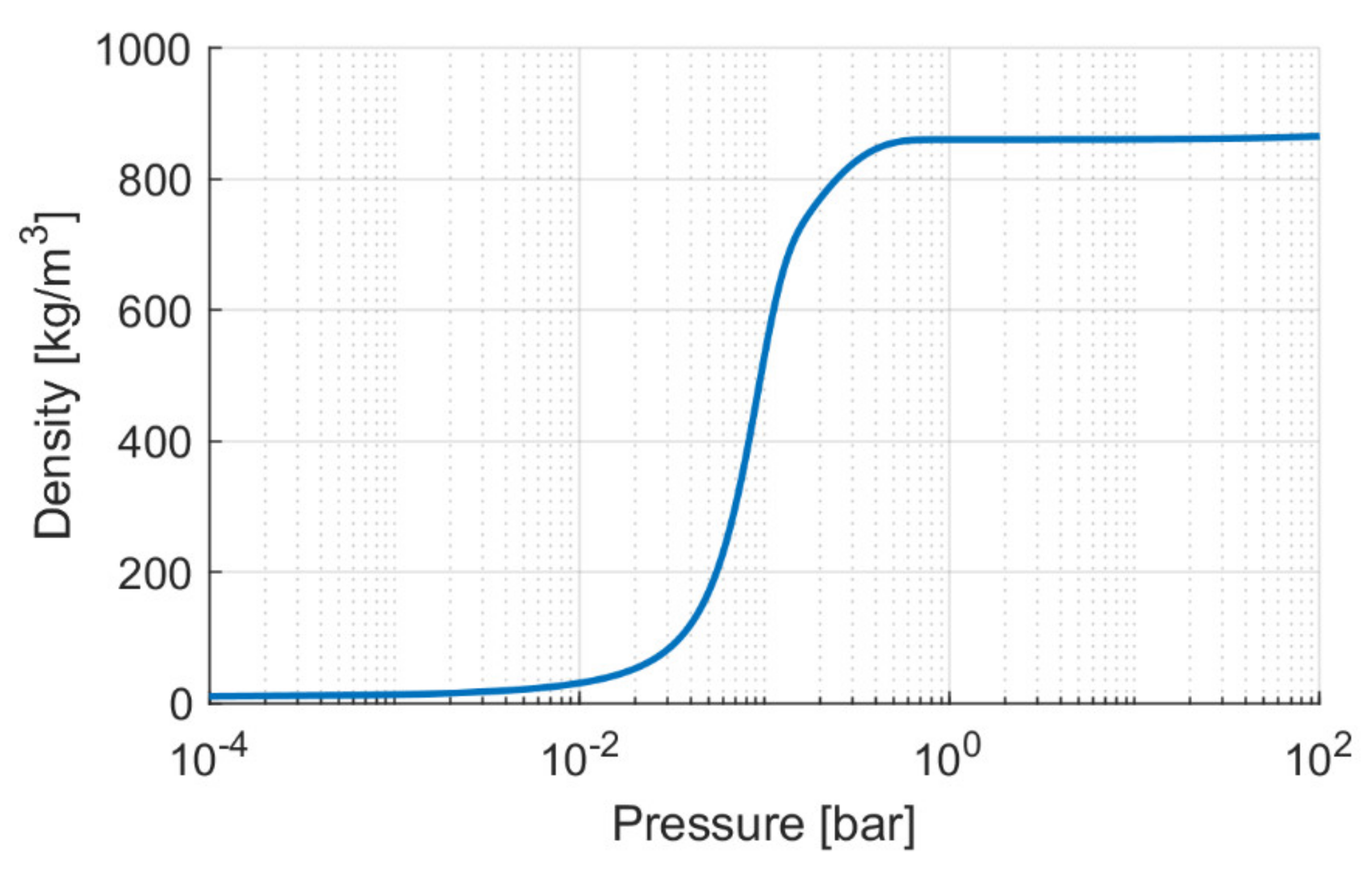
Figure 1 shows the density of the fluid as a function of pressure. Once the saturation pressure is reached, the density decreases markedly due to the release of the air contained in the liquid; once all the air is released, the density decreases further as a result of the gradual formation of vapor.
Adopting this model to predict the mass flow through a throat where the total pressure at inlet is
pT and the downstream pressure is
pS, the ideal fluid velocity at the throat is calculated as
for
p > psat the integral is analytically solvable and leads to
In the other cases the integral must be solved numerically.
This velocity value must be compared with the speed of sound at the static downstream pressure
where
and
The correct value of the velocity to be used for the calculation of the mass flow rate is the minimum between the speed of sound and the ideal velocity given by the Equation (15).
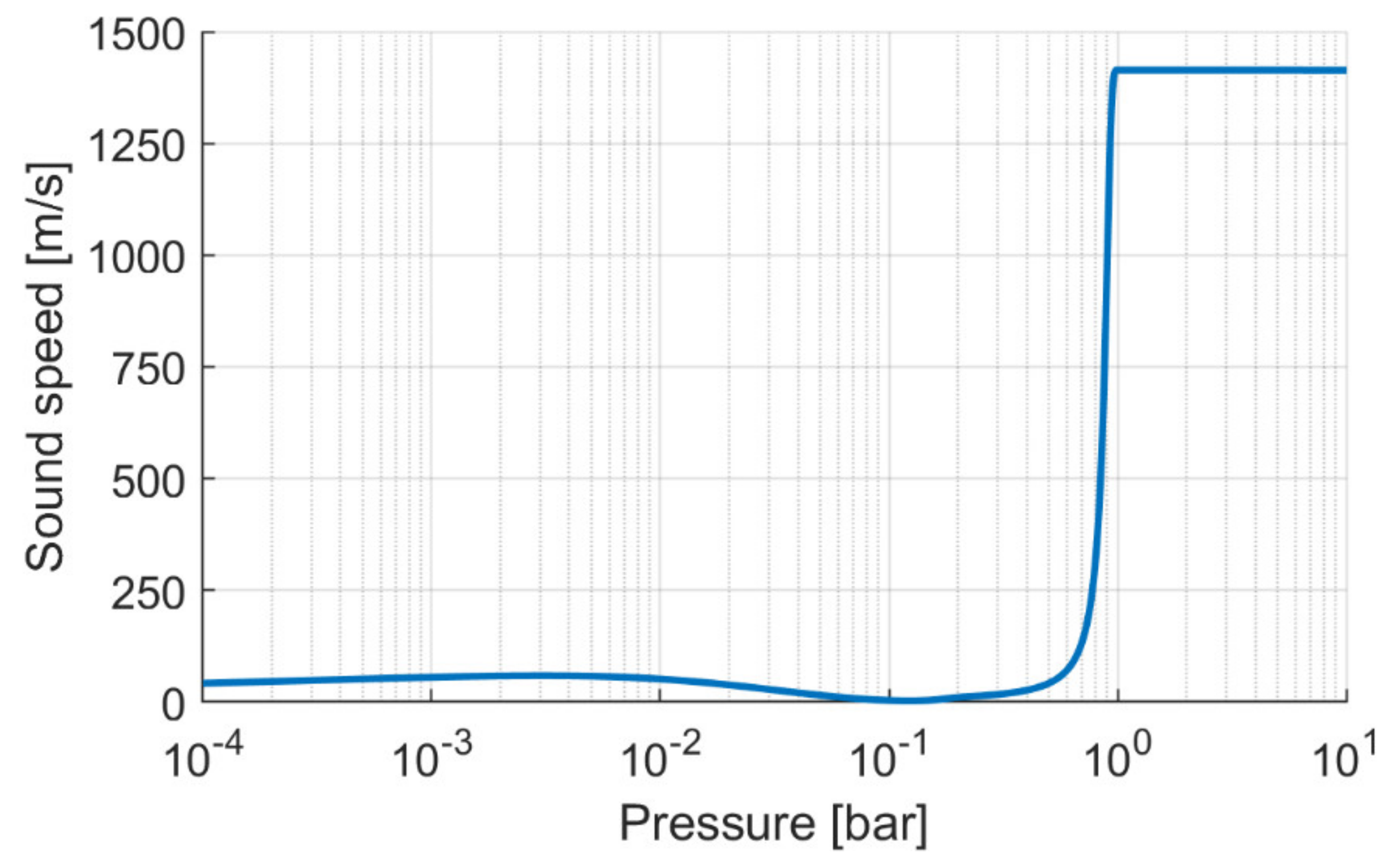
The trend of the speed of sound, calculated by means of Equation (17), is reported in
Figure 2. In general, it is a very high value, but as it is possible to see from the graph, for low pressures, such as the values involved in cavitation, the speed of sound decreases markedly; it is exactly in this pressure range that it is necessary to compare it with the ideal speed calculated with Equation (15).
4. Experimental Activity
The experimental activity was conducted at the test rig located in the Laboratory of the Engineering and Architectural Department at the University of Parma.
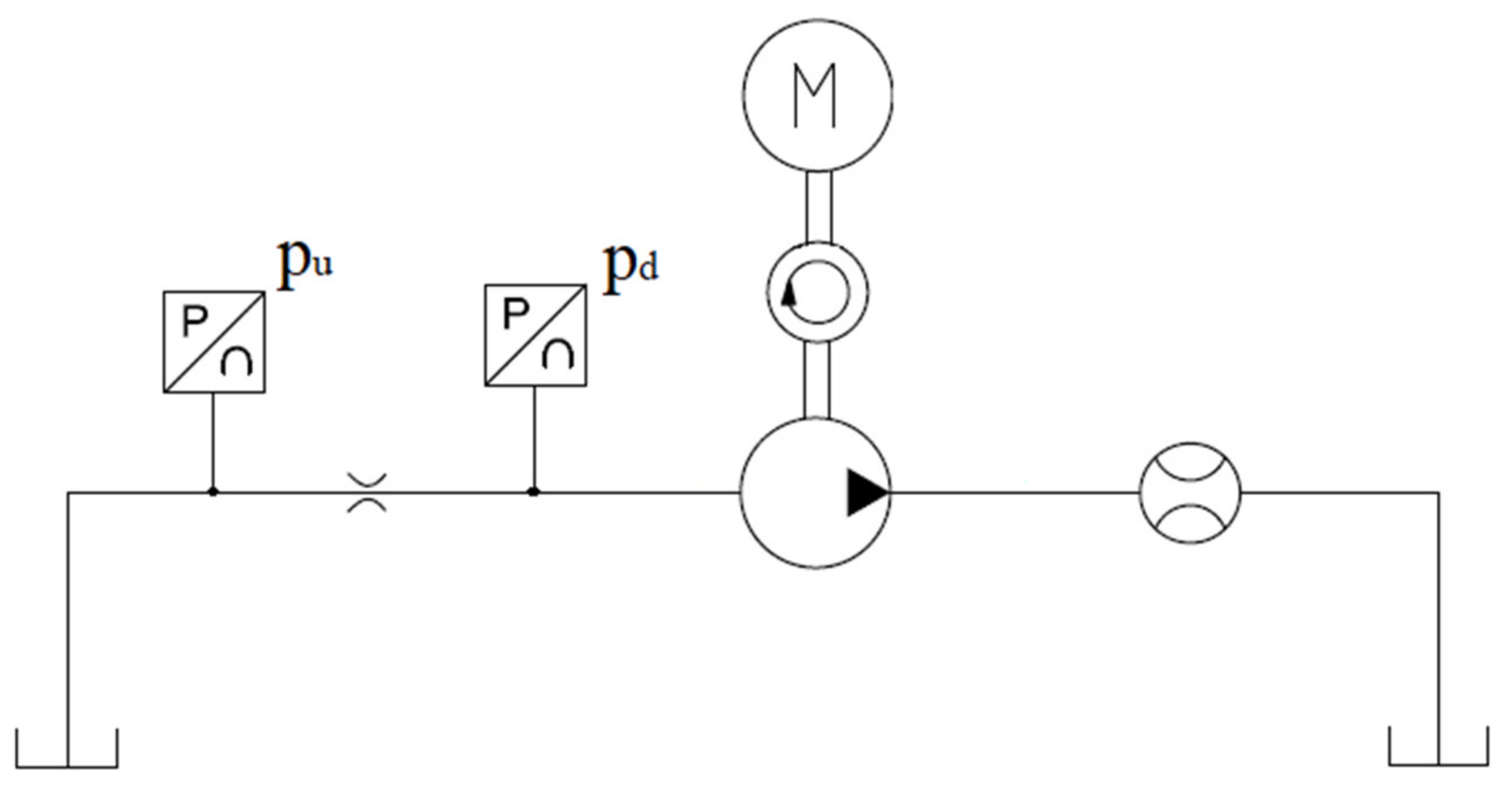
The hydraulic scheme of the experimental layout is reported in
Figure 3, and the transducers’ features are shown in
Table 2. The oil is an ISO-VG 46, and the test temperature was set to 40 °C.
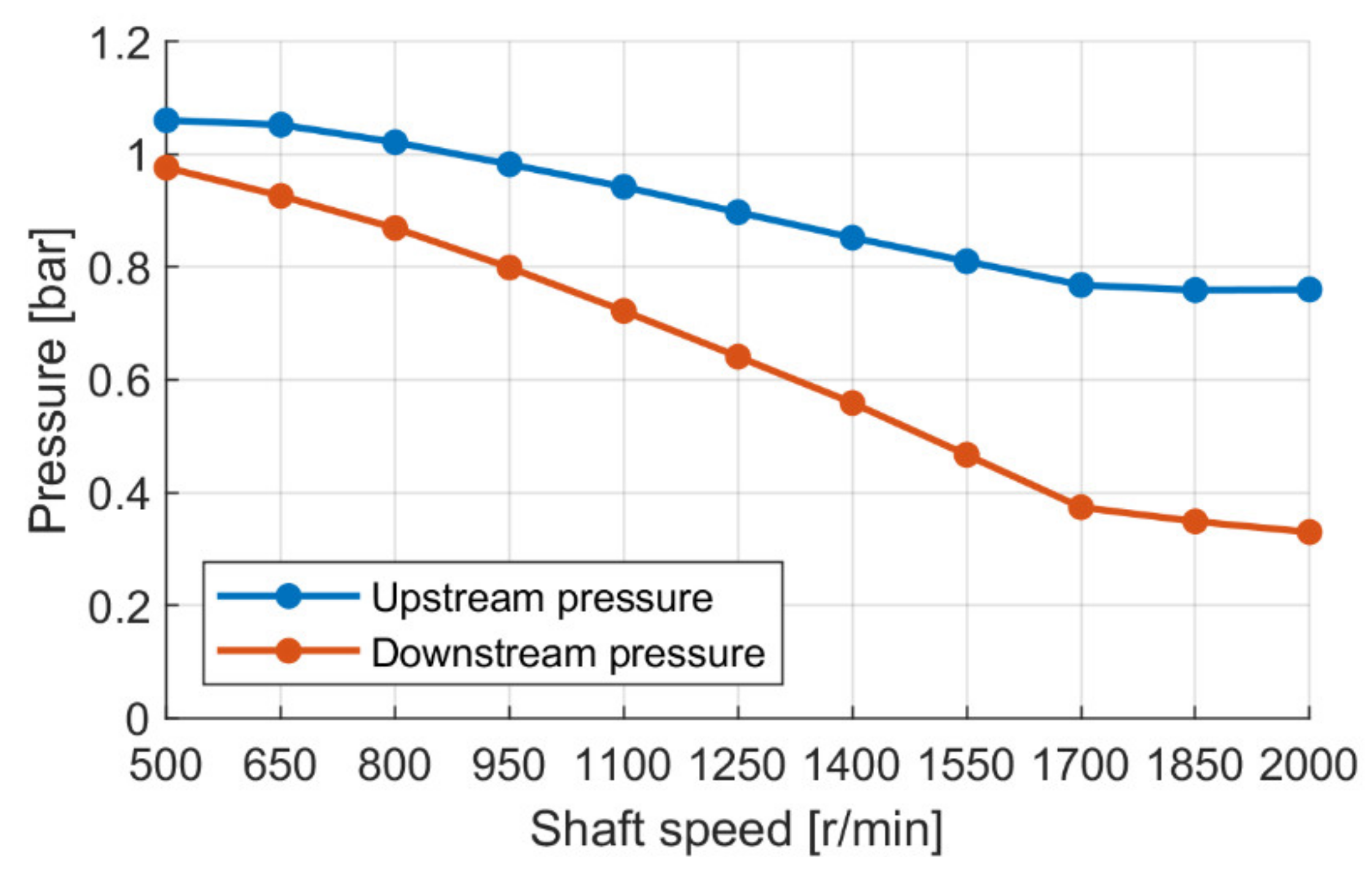
A fixed orifice was installed upstream of the pump in order to generate a pressure drop and to provide a low pressure value at the pump inlet. The pressure drop was given by the fluid velocity passing through the orifice and was controlled by the rotational speed of the pump. In order to accurately calibrate the parameters of the CFD model, the flow rate passing through the circuit and the absolute pressures upstream and downstream of the orifice were measured.
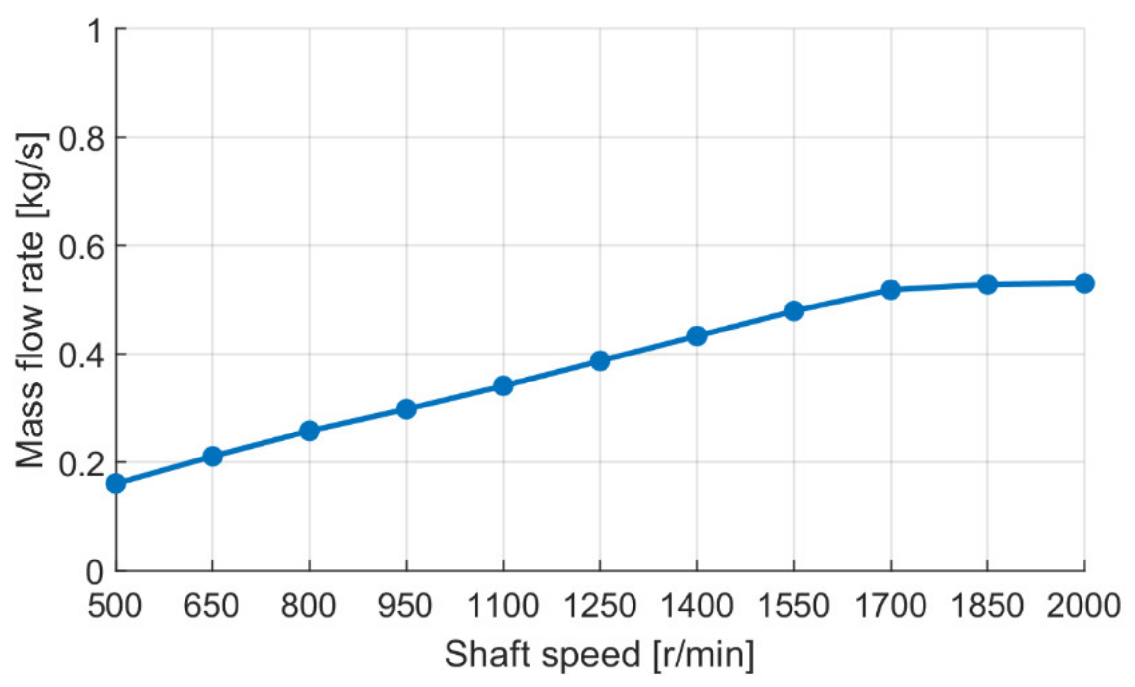
Figure 4 shows the flow rate measured by the flowmeter as the rotational speed increases.
In particular, up to 1550 r/min, the flow rate increased linearly with speed, and in this operating range, the main phenomenon was the release of a fraction of the dissolved gas; by further increasing the speed, the flow rate remained constant, and this was in accordance with what is also reported in [
14]. In fact, the pressure drop across the orifice did not increase much because the phenomenon of vaporous cavitation was established, which limited the minimum pressure reached downstream of the orifice, as can be seen in
Figure 5.
5. CFD Simulations
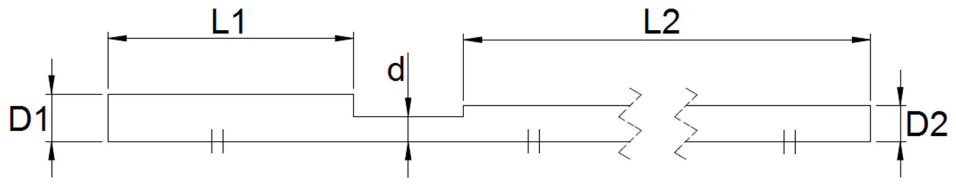
The geometry of the pipe is shown in the
Figure 6, where the length of the channel corresponds to the distance between the two pressure sensors, and the main geometric relationships are shown in the
Table 3. Since the geometry is axisymmetric, 2D geometry was used in the CFD simulations.
The simulations were done with ANSYS® CFX software. The gas cavitation model is not present in CFX, but it was implemented through the CFX Expression Language (CEL). CEL is a scripting language inside the main CFD code that allows operations on additional user-defined variables to be performed.
The fluid domain consists of a structured mesh, whose number of cells was established following a sensitivity analysis. The main features of the mesh are shown in
Table 4.
The turbulence model used is the standard k-epsilon. The absolute pressures measured by the sensors during the experimental activity were imposed as boundary conditions at the inlet and outlet. The upper wall was considered as a wall with a no slip condition, while the symmetry boundary was imposed on the front plane where the axis of symmetry was the one indicated in
Figure 6.
In
Table 5, the parameters used in the model are reported. Two sets of parameters reported differ in the vaporization coefficients. Zhou et al. [
4] proposed the values of Set A, studying gaseous cavitation by applying a model of vaporous cavitation in a hydraulic circuit with an orifice inside. These values were also reported in the research of Del Campo et al. [
10], who studied the phenomenon of gaseous cavitation in external gear pumps. These values were also adopted in a previous work [
11], where the influence of cavitation on textured surfaces was studied. Generally, the vaporization coefficient is greater than the condensation one, because condensation is a process that occurs more slowly than vaporization, and this aspect is quantified with the
Fc and
Fv parameters.
The air release and absorption model is quite innovative, and in the literature there are only applications with water with the values shown in the table. However, it was decided to use these values because, as will be seen in the simulation results, they allowed good correspondence with the experimental data to be obtained. The absorption constant Ca is smaller than desorption constant Cd for two reasons. The absorption process has to overcome surface tension effect, which opposes higher resistance; and the pressure differential during the air release is bounded by the maximum value of pequil, while it is unbounded during absorption.
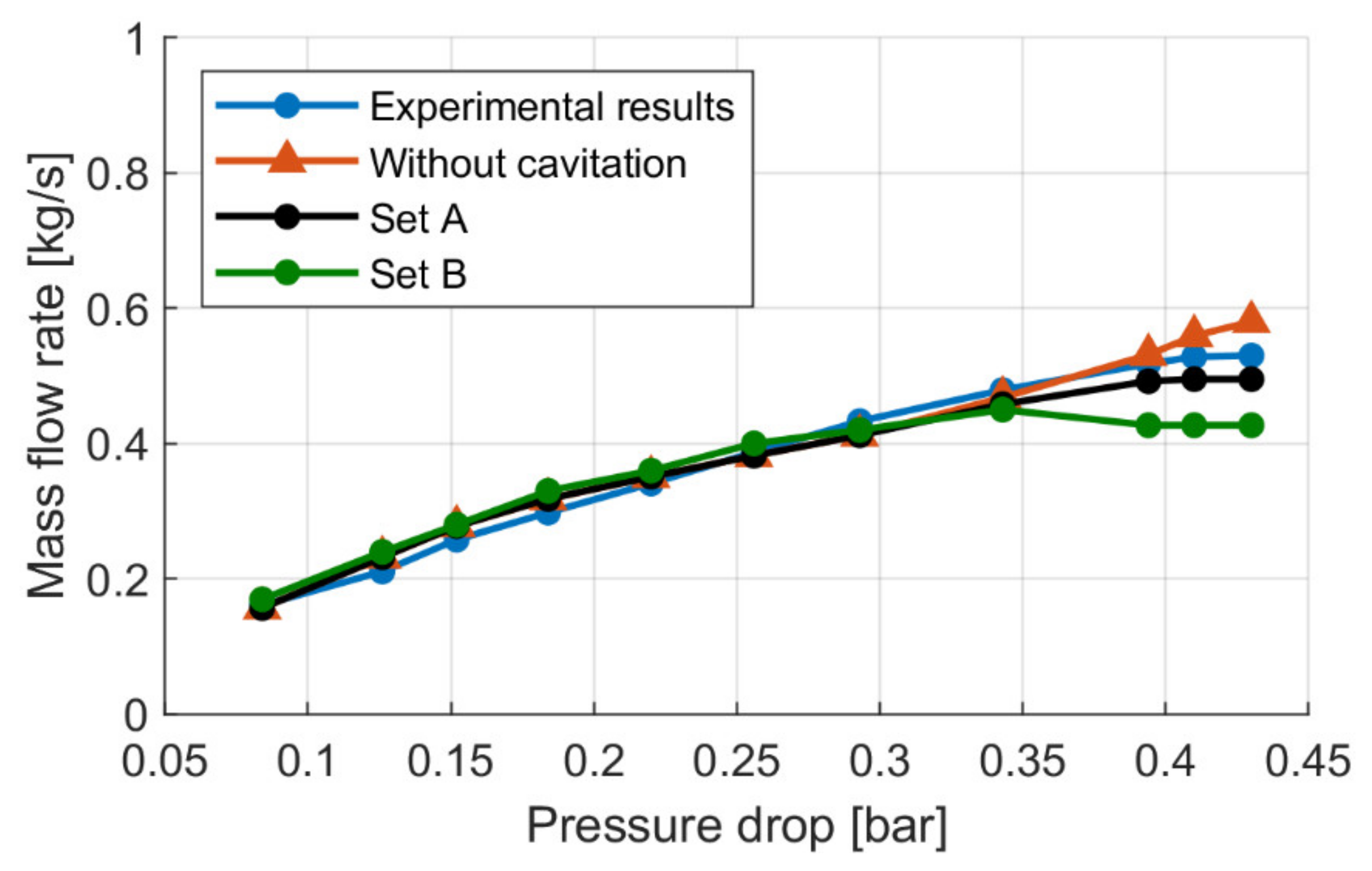
Figure 7 shows the mass flow rate through the orifice obtained from the CFD simulations, compared with the experimental results as a function of the pressure drop. The graph shows the simulation results obtained with the two sets of parameters; as long as the pump speed does not exceed 1500 r/min, the pressure drop across the orifice is not enough to generate vapor. In the first part of the graph, therefore, the results of the two sets of parameters are equivalent. At higher pressure drops, however, vapor is also formed, and therefore the vaporization parameters greatly influence the calculated flow rate. Since Set B has a higher vapor formation coefficient than Set A, it involves a greater quantity of vapor, which leads to a lower estimation of the flow rate passing through the orifice. Therefore, the most accurate of the two sets of parameters results is Set A, since it is possible to appreciate a good overlap of the two curves, especially where the flow rate settles and the vapor cavitation is predominant.
Since the parameter Set B underestimates the flow excessively at high speed, the following results are relative to Set A.
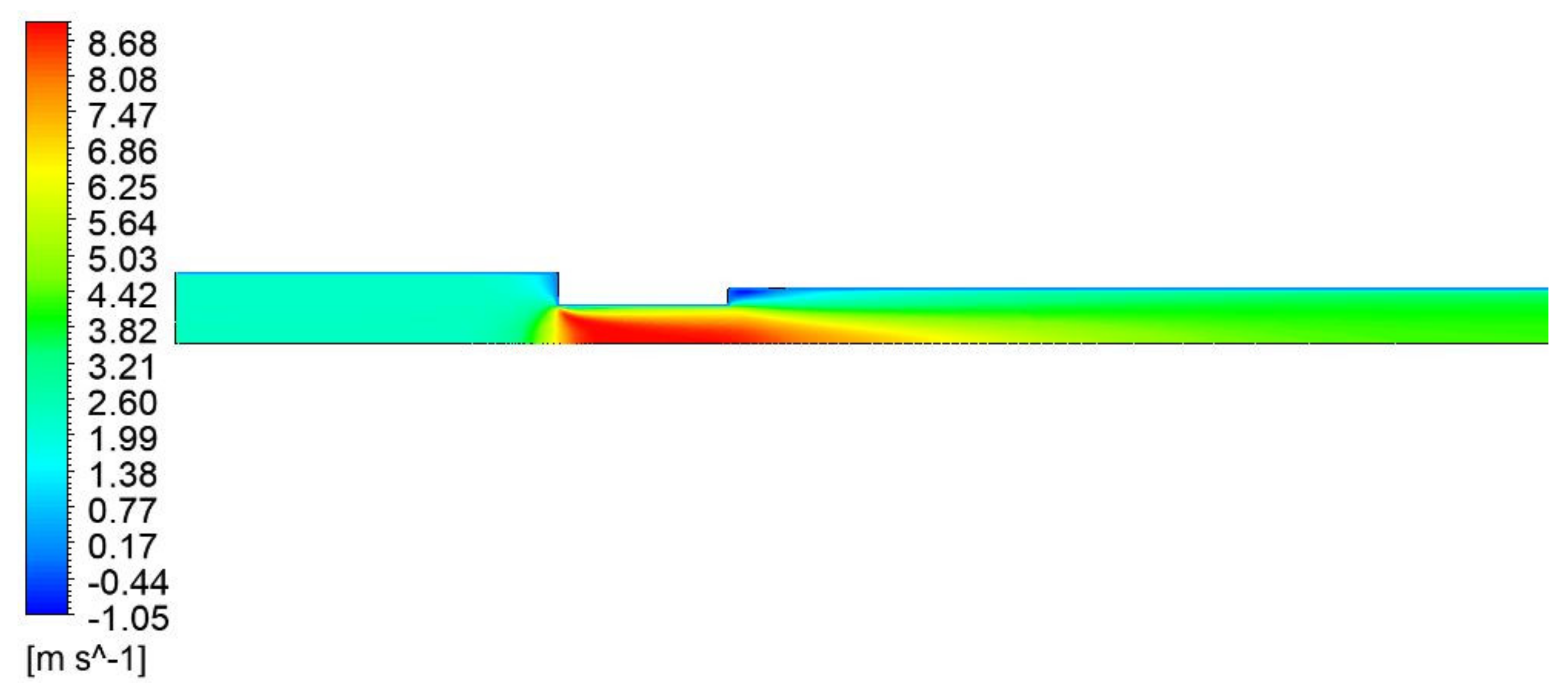
Figure 8 shows the oil speed distribution in the geometry considered in the case of a pressure drop of 0.256 bar; it is important to observe the speed distribution, since it has consequences on the results in terms of pressure distribution and on the formation of the gaseous phases (both air and vapor).
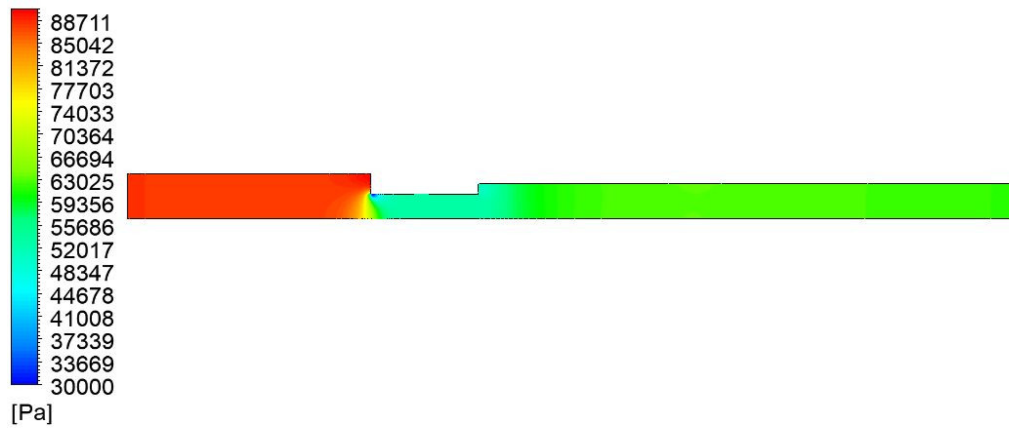
Figure 9 shows the pressure distribution relative to the case of a pressure drop of 0.256 bar. Near the orifice, where the section is convergent, there is a minimum due to the greater velocity of the fluid. Further downstream, the pressure tends to increase because of the reduction in fluid velocity and the consequent conversion of kinetic energy into pressure.
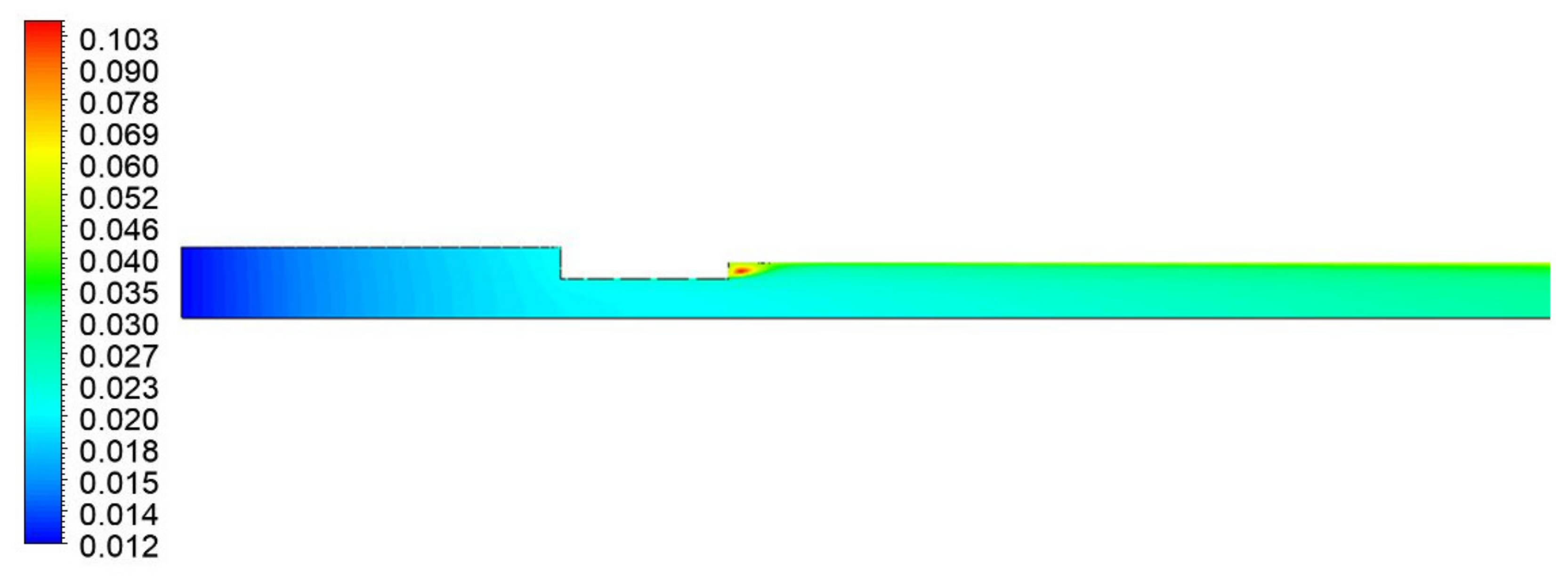
The
Figure 10 shows the volume distribution of free air. The greater quantity is concentrated in the divergent section since this represents a stagnation area; the fluid velocity, as seen in
Figure 8, is negative and contributes to increase its concentration in this area.
In this condition, the minimum pressure to also have vapor formation is not reached. By increasing the pressure drop across the orifice, the minimum pressure reached is such as to trigger the formation of vapor. In
Figure 11, it is possible to note that the minimum pressure is the one set as vaporization pressure.
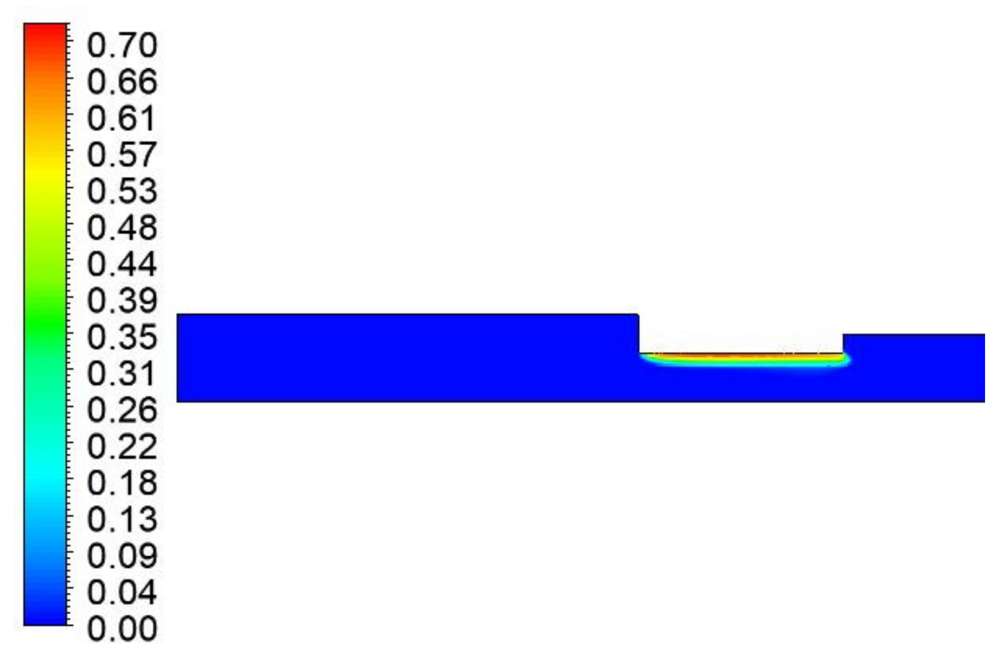
Figure 12 shows the volume fraction of vapor that is formed in the domain: when the downstream static pressure drops, a region of fluid in the vapor phase forms inside the restriction which narrows the effective section where the fluid flows.
6. Lumped Parameter Model Results
Experimentally, the downstream pressure was acquired distant from the orifice, but in order to correctly apply the orifice equation it is necessary to know its value near the outlet section, which is calculated thanks to CFD simulations.
To calculate the flow rate passing through the orifice, the following equation is used:
where
Ω is the orifice cross sectional area. The density value
ρ used was obtained from
Figure 1 at the orifice downstream pressure.
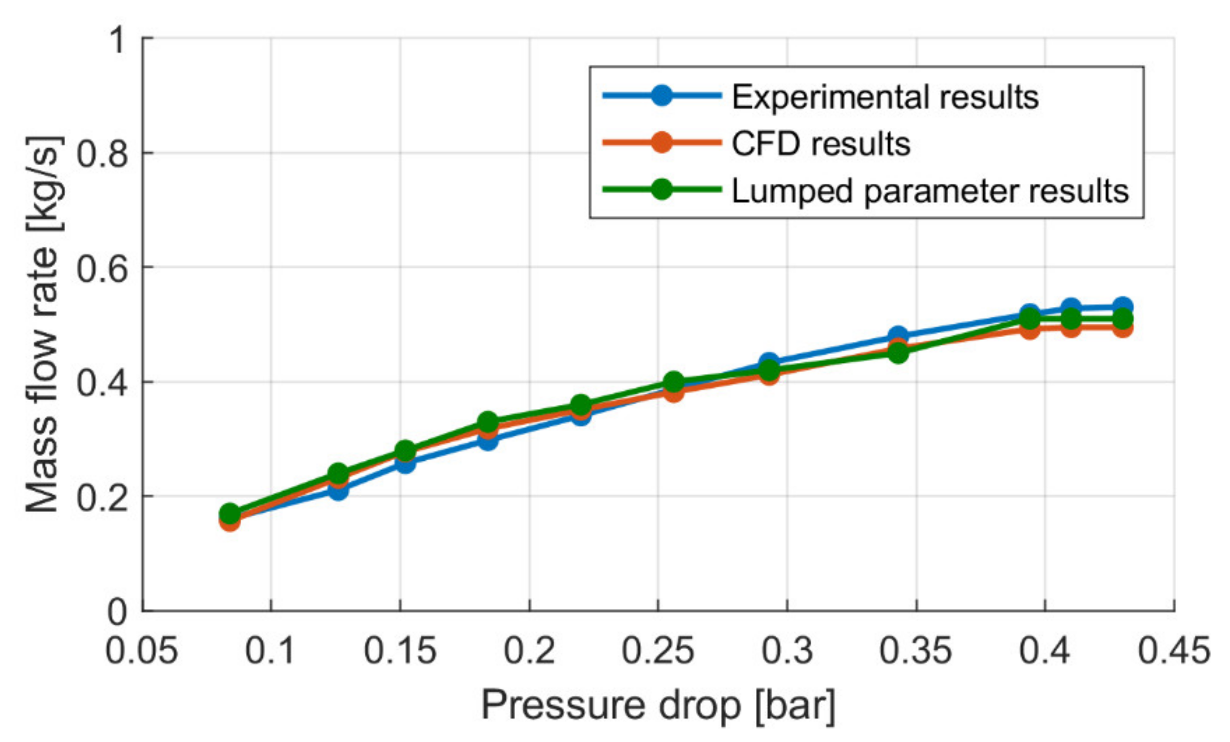
Figure 13 shows a comparison between the experimental results and those obtained from CFD simulations and with the lumped parameter method. As well as the CFD results, the lumped parameter model also predicts the mass flow rate with good accuracy; in fact, the maximum deviation between the experimental data and the results of the CFD simulations was 7%, while the maximum deviation between the experimental data and the lumped parameter model was 6.4%.
To obtain the results shown in
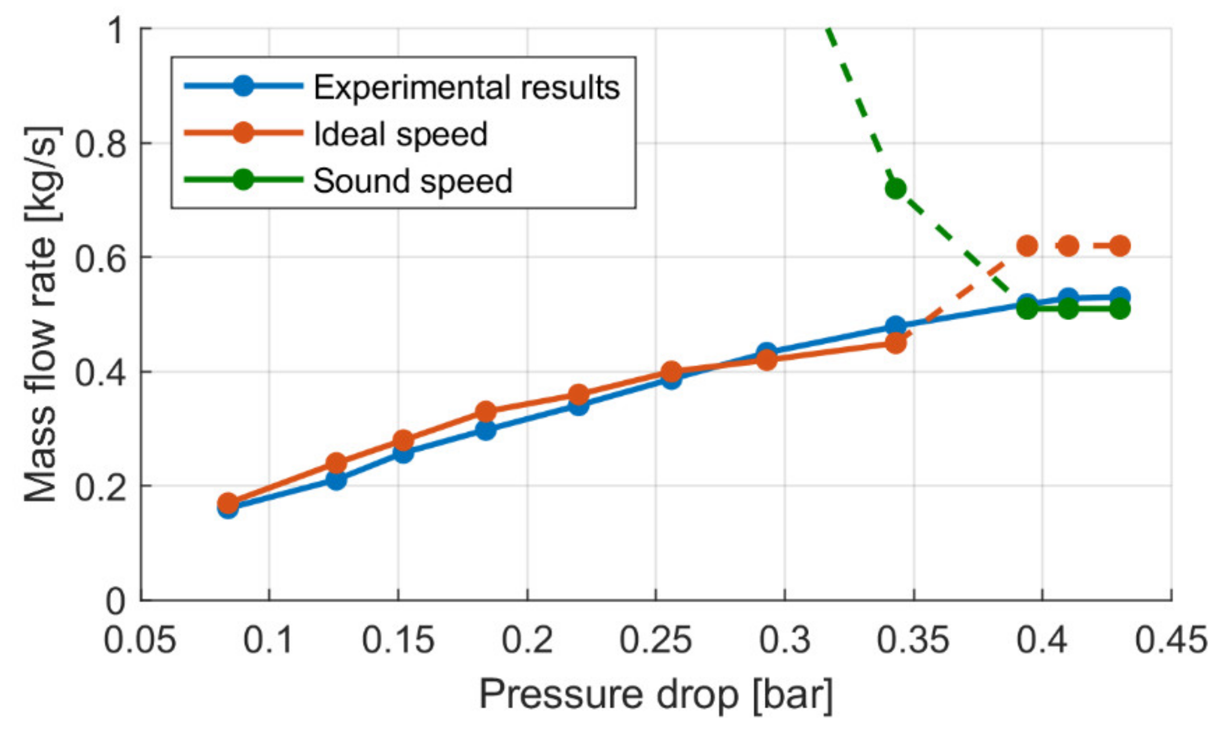
Figure 13, it is essential to use the correct flow speed value, the
c term in Equation (23), given by the comparison between the ideal speed, Equation (15), and the speed of sound, Equation (17). The use of the expression of the ideal speed in the entire range involves an important overestimation of the mass flow passing through the orifice when vapor cavitation develops (pressure drop greater than 0.34 bar), as seen in
Figure 14. However, when a greater pressure drop is generated, the condition where the ideal speed exceeds the speed of sound occurs, represented by the dashed red line. In this case, the speed that should be correctly used is the speed of sound, indicated by the solid green line, while the dashed green line represents the mass flow rate calculated with the speed of sound at a smaller pressure drop. The results show that the mass flow rate predicted by the model corresponded with the experimental one using the ideal speed up to a pressure drop of 0.34 bar and the speed of sound for higher shaft speeds.
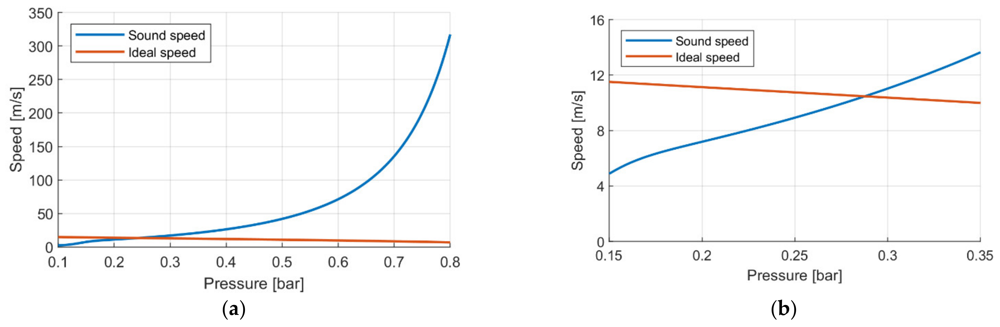
Figure 15 shows two graphs with the comparison between the ideal speed of the fluid and the speed of sound. The first graph,
Figure 15a, relates to a total upstream pressure of 1.05 bar; this is the case of a pressure drop of 0.08 bar, and the ideal speed is well below that of sound. This case is representative of conditions up to a pressure drop of 0.34 bar. At even a higher pressure drop, the total upstream pressure is reduced, and the two speeds, ideal and sound, become comparable (
Figure 15b), and when vapor is formed, the ideal speed is greater. To correctly calculate the mass flow rate, it is therefore necessary to use the value of the speed of sound.
7. Conclusions
This paper presents two models for predicting gaseous and vapor cavitation phenomena. One is based on a CFD approach and implemented in ANSYS® CFX in which an air release and absorption model is introduced, the other is a lumped parameter fluid model.
An experimental apparatus was realized to test cavitation in a hydraulic circuit where an orifice is placed on the inlet line of a pump, which serves to generate flow through the restriction.
The pressures measured by the sensors were used as boundary conditions in the simulations to obtain the measured mass flow rate through the orifice. The advantage of the CFD model is also to show where the gas phase is concentrated; this is fundamental, since the gaseous fractions represent a critical factor in the functionality of hydraulic systems. Once the CFD model was validated, the fluid dynamics simulations were necessary for the correct application of the lumped parameter model. The latter model also shows the need to correctly calculate the velocity of the fluid, not merely considering the ideal velocity but also comparing it with that of sound; otherwise, there is the possibility of overestimating the mass flow rate. The good level of correspondence with the experimental data shows the potential of both methodologies for the study of cavitation problems in hydraulic systems.
The outcome of this research will allow for the study of cavitation in hydraulic control valves or pumps through the proposed models.


