1. Introduction
In the lumped parameter modelling of fluid power components, some coefficients that play a critical role in the simulation are typically unknown and not easy to be determined or to be found in the open literature. Moreover, in hydraulic systems, nonlinearities are responsible for critical behaviors that make it difficult to realize a reliable mathematical model for the numerical simulation. In most cases, the unknown parameters of a complex simulation model of an entire hydraulic system are selected a posteriori in order to obtain a good agreement with a few available experimental data. However, with this approach, the predictive capability of the model could be compromised, and its reliability in evaluating quantitatively the influence on the system performance of a parameter modification could be questionable, especially if the number of the unknown coefficients is high. In fact, it is possible that the same global behavior of the system could be obtained with different sets of coefficients; therefore, the real weight of some parameters may not be properly caught. In order to avoid this limitation, the best procedure, when possible, is to characterize as best as possible the single components with focused tests. In this way, the reliability of the system-level model can be improved.
With specific reference to continuous position fluid power valves, two types of coefficients are often difficult to be known with good accuracy: the discharge coefficient of the flow area, and the friction coefficient between the spool (sliding body) and the housing. The influence of the former is less critical due to the quite limited range of variation, typically between 0.6 and 0.9, even if in some specific applications such a variation can nevertheless have a significant impact on the predicted system performance [
1]. On the contrary, an incorrect definition of the friction coefficient value can lead one to predict erroneously system instability when the system is stable, and vice versa, due to a wrong representation of the physical phenomenon [
2].
The knowledge of the dynamic friction behavior becomes relevant when a friction compensation strategy is implemented in the control systems, as reported in [
3,
4] for an electro-hydraulic excavator.
Generally, the friction force between a body sliding within a fixed casing has a nonlinear characteristic as a function of the relative speed. In this paper, only the viscous friction that is the main phenomenon affecting the investigated component is analyzed. As a matter of fact, no load is applied in the direction perpendicular to the spool axis, given that the radial forces are almost completely compensated; therefore, it is reasonable to assume that the lubricant film is thick enough to support the sliding body, and dissipations are due only to viscous losses [
2]. Furthermore, there are other examples of hydraulic valves where only the viscous friction coefficient (speed dependent) is important, while the Coulomb friction (pressure dependent) can be neglected. This is the case, for instance, where the diether effect of a PWM (pulse-width modulation) control keeps the spool always in oscillation around an equilibrium position [
5]. Moreover, all spools of the hydraulic valves are provided with annular grooves [
6] for the radial balancing in order to minimize as much as possible the stick–slip phenomenon.
With reference to fluid power components in general, the scientific literature reports analysis of dynamic friction considering a hydraulic cylinder under various conditions of velocity; in the case considered in [
3], the stick–slip phenomenon has been investigated; it is reported that when the sliding component starts to move again after a short dwell time, the force required is much smaller with respect to what found after a long dwell time. An explanation is found in the decrease of the lubricant film thickness, which is much smaller when the time at zero velocity is negligible.
In this paper, the investigated component is a part of a pump displacement control, where the sliding component oscillates continuously around an equilibrium position, and therefore the dwell time is very little, making the stick–slip phenomenon irrelevant. The component investigated in this paper has a key role in controlling the instantaneous displacement of an axial piston pump [
7,
8,
9]. The authors have developed models of the pump [
10] and of the hydraulic system for an excavator [
11,
12,
13,
14], where the pump with its displacement control is installed, a reliable model of the control permitted to correctly simulate the pump behavior during the transients that characterized the typical duty cycle of an excavator. To the best authors’ knowledge, no experimental procedure is available in the open literature for the characterization of the viscous friction coefficient in such displacement controls. The values usually utilized by the scholars in their simulation models come from simplified theoretical hypotheses, such as the perfect coaxiality between the movable element and its seat. On the other hand, an experimental measurement needs a very specific “non-intrusive” approach, above all for small valves, on a dedicated test bench.
In this context the current paper presents two methodologies to assess experimentally the viscous friction coefficient that can be applied for any kind of hydraulic spool valve characterized by working conditions in which the dwell time between acceleration and deceleration of the spool is very small to make the stick–slip phenomenon not relevant. The methodologies reported in this paper are mainly based on experimental tests to collect data that can be used in the presented mathematical models to define the value of the viscous friction coefficient. The authors point out that the two methodologies were developed in two distinct laboratories in different periods of time; later, the authors have discovered that the outcomes were coincident, notwithstanding that the followed approaches were completely different. Hence, the importance of presenting in the same paper both methodologies is to demonstrate their mutual validation, since no other standard approach is available. One of the approaches was carried out at the Fluid Power Research Laboratory of the Politecnico di Torino (Turin, Italy), while the other was developed at the University of Parma (Italy). Both methods are based on the generation of a pressure oscillation and the dynamic measurement of the pressure in two different points of the test circuit. The signals were used to calculate the transfer function that relates the two pressures. The same function was also calculated thanks to a simulation model of the component, with which the value of the viscous friction coefficient that permits the best agreement between experimental and numerical data was determined. Both proposed methods do not require the installation of a spool displacement transducer that can significantly affect the results; this aspect has also been investigated, and the outcomes are presented in this paper.
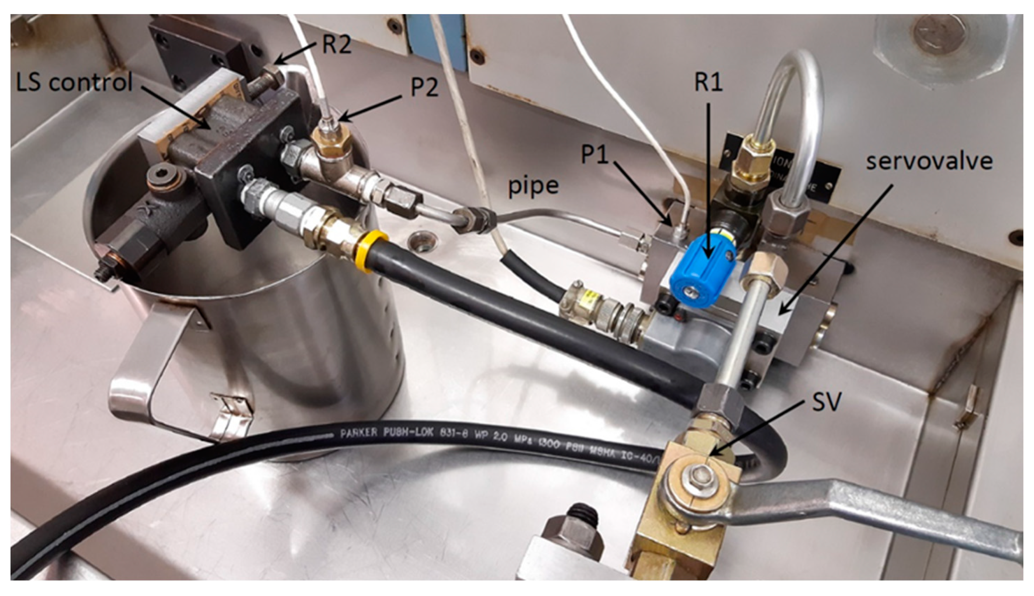
The first methodology is based on the use of a servovalve for generating pressure oscillation at the inlet of a small pipe connected to the pilot chamber of the valve under test. The transfer function relates the pressures at the two ends of the pipe, and it is influenced by the oscillations of the spool. The second methodology developed at the University of Parma is based on experimental tests where the spool oscillations generated by the pressure ripple of a pump at the inlet port of the valve under test causes a time dependent flow rate at the outlet. The measurement of the fluid pressure both at the inlet and at the outlet of the component has permitted the transfer function to be defined. Therefore, not only the methods differ for the means of generating the oscillation of the spool, but also in the path of the fluid analyzed. In the first method, only the pilot line is considered with the valve ports closed, while in the second, the main flow through the valve is considered.
The paper is organized as follows: In
Section 2, the tested component is described; in
Section 3 the mathematical model concerning the first method is presented, to demonstrate the correlation between the measured fluid pressure and the viscous friction coefficient; in
Section 4 the second method is presented mainly focusing on the experimental setup; a final discussion is reported in
Section 5.
2. Description of the Tested Component
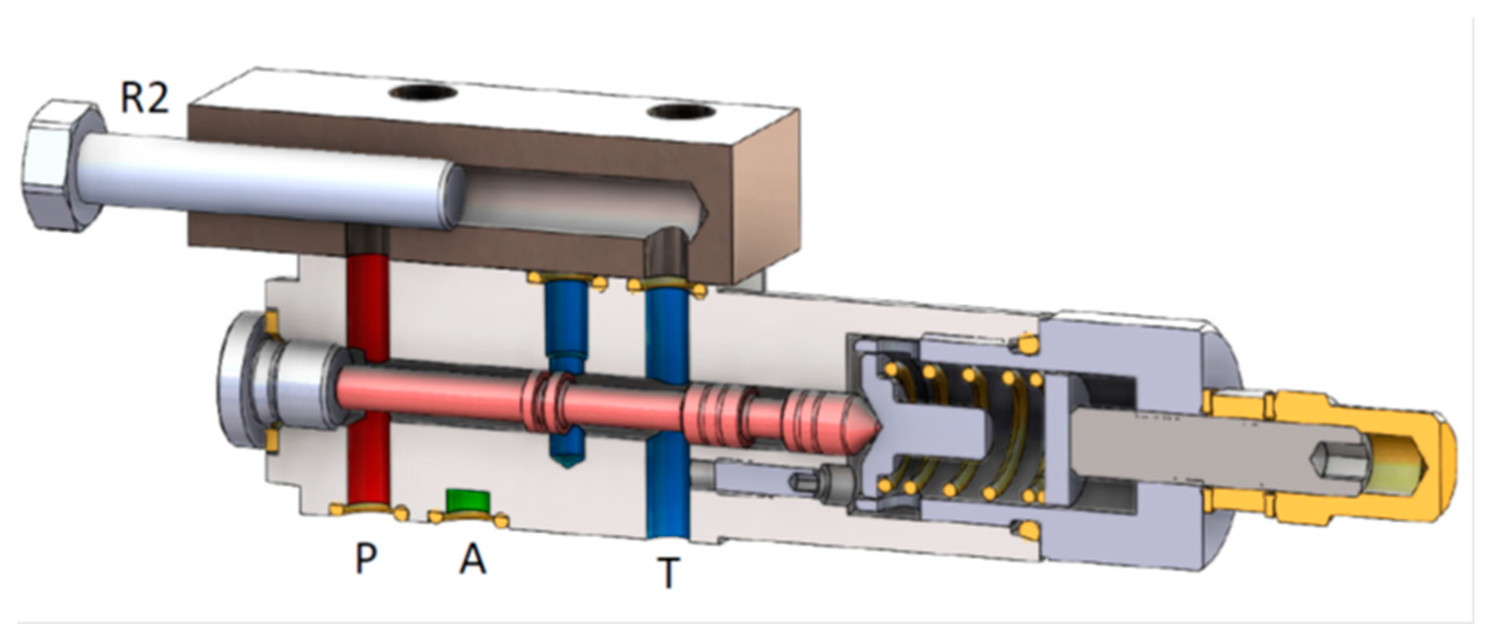
The proposed methodologies were applied to a flow compensator (FC) that in a load sensing system has the function of regulating the flow rate by acting on the pump displacement. The logic governing the FC is to compare the maximum load pressure (pLS) of the hydraulic actuators with the pump delivery pressure (pS). In particular, the analyzed FC is mounted on an axial piston pump, and it has the function of regulating the swash plate angle.
In
Figure 1 a simplified hydraulic scheme for feeding a single actuator is shown. The FC is a small three-port continuous position pilot valve, where the spool position depends on the pressure levels p
S and p
LS and on the force of an adjustable spring. The pump displacement is a function of the equilibrium of two actuators 1 and 2 with different diameters. The smaller actuator 2 is always connected to the delivery pressure, while the pressure acting on the larger actuator 1 is modulated by the FC. When the FC is not regulating (control in saturation), the actuator 1 is connected to the atmospheric pressure, and the actuator 2 holds the maximum pump displacement. On the contrary, when the valve spool is in equilibrium in an intermediate position, the pressure in the piston 1 is increased, its exerted force is able to balance the force of the piston 2, and the pump displacement is reduced. The condition of equilibrium of the spool implies that the delivery pressure p
S is maintained equal to the load sensing pressure p
LS incremented by a contribution given the adjustable spring, typically around 20 bar. In this way the FC maintains a fixed differential pressure across the main control valve, represented in the scheme by a variable restrictor CV, so that the flow rate delivered to the actuator depends only on the flow area of CV and not on the load pressure p
LS.
Since a load sensing system is intrinsically closed loop pressure controlled, where the pilot line for transferring the load pressure p
LS represents the feedback signal, it features poor behavior in damping high inertial loads [
15]. Hence a possible risk is the instability that is also influenced by the viscous friction force of the FC. It is desirable that a simulation model of the hydraulic circuit could be able to predict the instability, but if the real damping coefficient of the spool of the FC is unknown, the reliability of the model for such a study could be questionable. For this reason, the spool of a load sensing pressure compensator represents a good example of application of the proposed methods for the measurement of the viscous friction.
4. Second Method
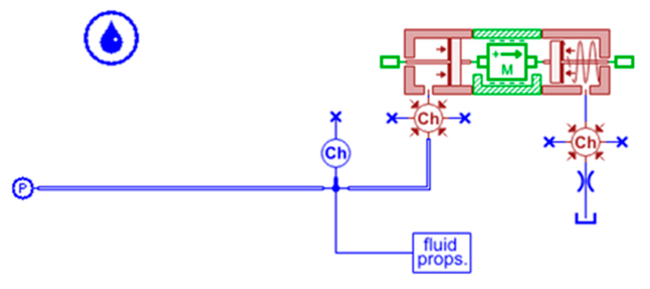
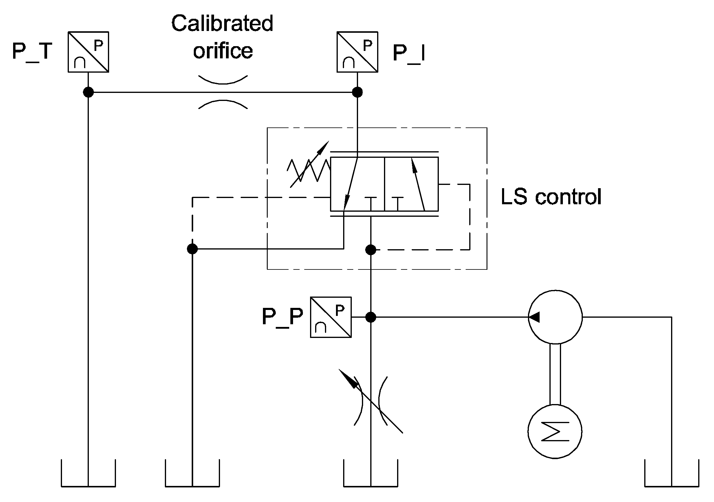
In this section, the second methodology to define the value of the friction coefficient is presented. This approach is mainly based on experimental tests where the component has been excited in order to evaluate its dynamic response. Additionally, this methodology permits the component to be kept unchanged without the addition of a spool displacement transducer that changes the mass of the spool in a significant manner and adds further friction losses due to the spool of the transducer. In this second methodology, the use of a servovalve is not necessary, but a cheaper gear pump was used to excite the component. The ISO scheme of the circuit is reported in
Figure 15.
The component was connected to the delivery line of a gear pump, the flow ripple of which generates a pressure ripple that dynamically excites the spool of the component. As is well known, it is not possible to measure a flow ripple with a high bandwidth instrument, unless using complex and indirect methods [
17]; therefore, the fluid pressure ripple at the inlet of the component was acquired during the tests. The fundamental frequency of the pressure ripple (P_P) depends on the pump speed that can be easily changed during the tests, and then the spool can be excited at different conditions. The spool oscillations generated by the pressure ripple cause a time dependent flow rate at the outlet (line I) that once again cannot be measured. As reported in
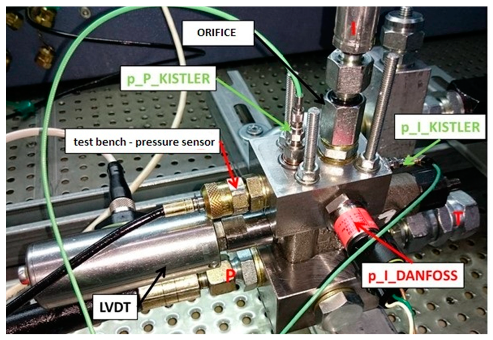
Figure 15, a calibrated orifice was introduced along the return line for converting the flow ripple in a measurable pressure ripple (P_I), and the size of this orifice was defined after several tests with different size diameters. The target was, on one hand, to generate an average pressure level to avoid too low minimum values; on the other hand, the average pressure could not be too high in order to neglect the effect of fluid compressibility. The pressure at the inlet (P) was set at an average value of 30 bar and 50 bar. The sensors were installed as close as possible to the component, and the entire layout was compacted to reduce the volume of fluid that could induce compressibility effects.
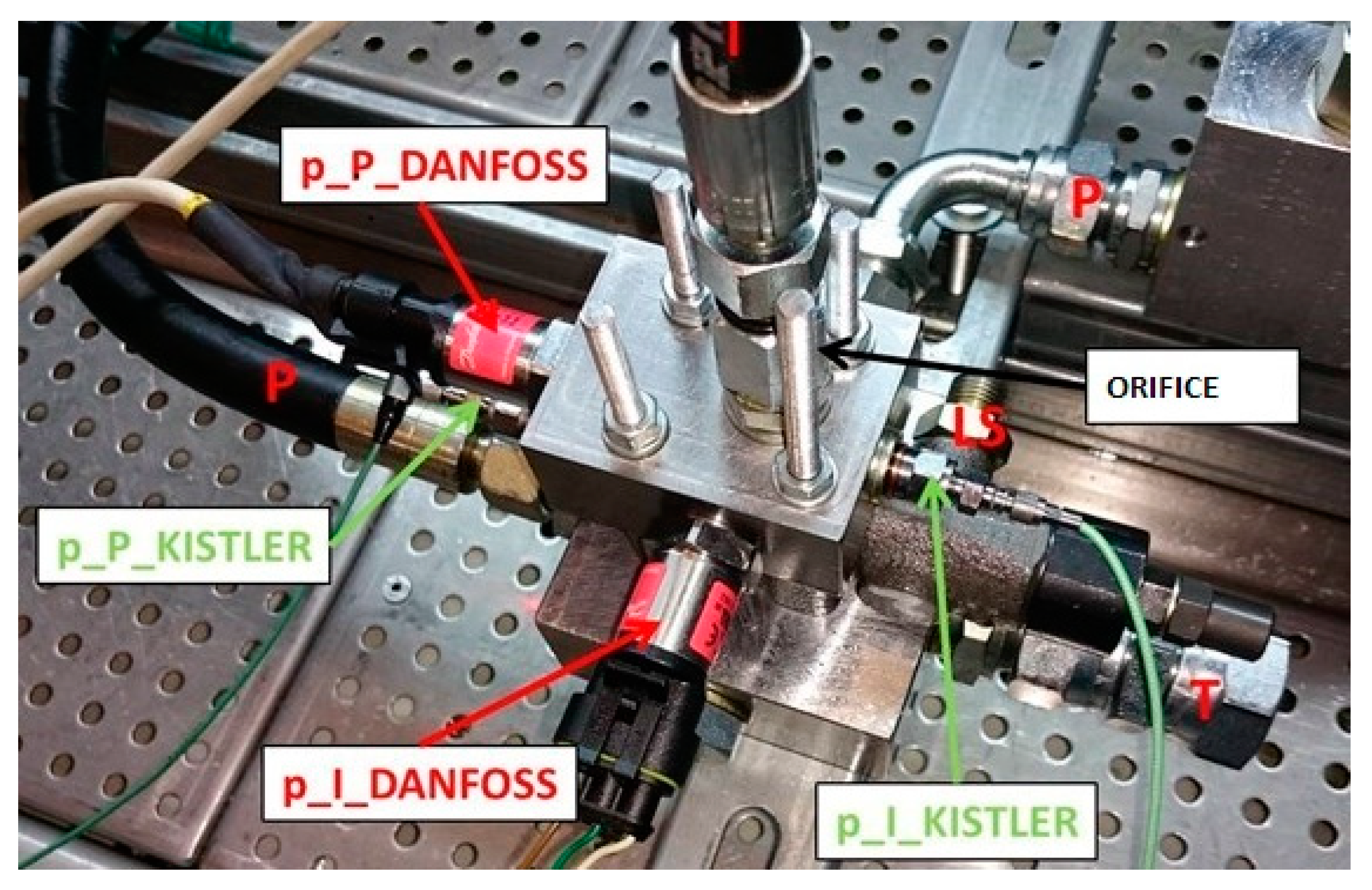
Figure 16 reports a picture of the component installed on the test bench with sensors. All tests were carried out by setting the fluid temperature equal to 40 °C.
In order to define the dynamic behavior of the component, the pressure oscillations at the inlet were assumed as “input data”, while the pressure oscillations at the outlet were assumed as “output data”. It is essential to acquire the pressure values at the inlet and outlet simultaneously; therefore, a double channel amplifier KISTLER
® 5064 was used together with the pressure transducers reported in
Table 2; the sampling rate was set equal to 20 kHz.
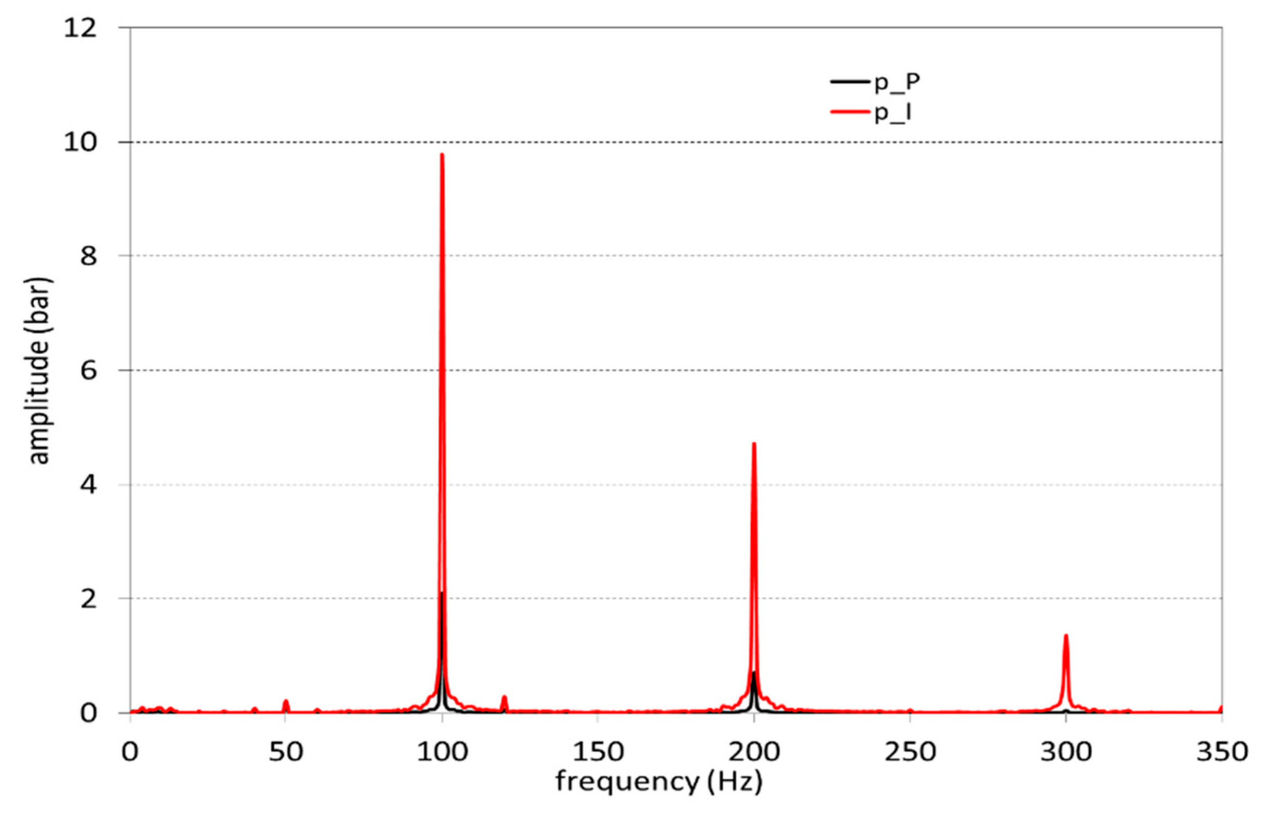
During the tests, the pump speed was changed from 120 rpm to 3000 rpm in order to cover the frequency range from 20 Hz to 500 Hz, being that the gear pump had 10 teeth. This range is suitable for the investigation, because the theoretical natural frequency of the component is about 300 Hz. In
Figure 17, the pressure oscillations measured at the inlet, P_P, and at the outlet, P_I, are reported with a pump speed of 600 rpm, which corresponds to the fundamental frequency of 100 Hz; the average inlet pressure was set to 30 bar and the calibrated orifice with a diameter equal to 1.2 mm. The Fourier transform of both signals are reported in
Figure 18, where the first harmonic at 100 Hz is clearly visible.
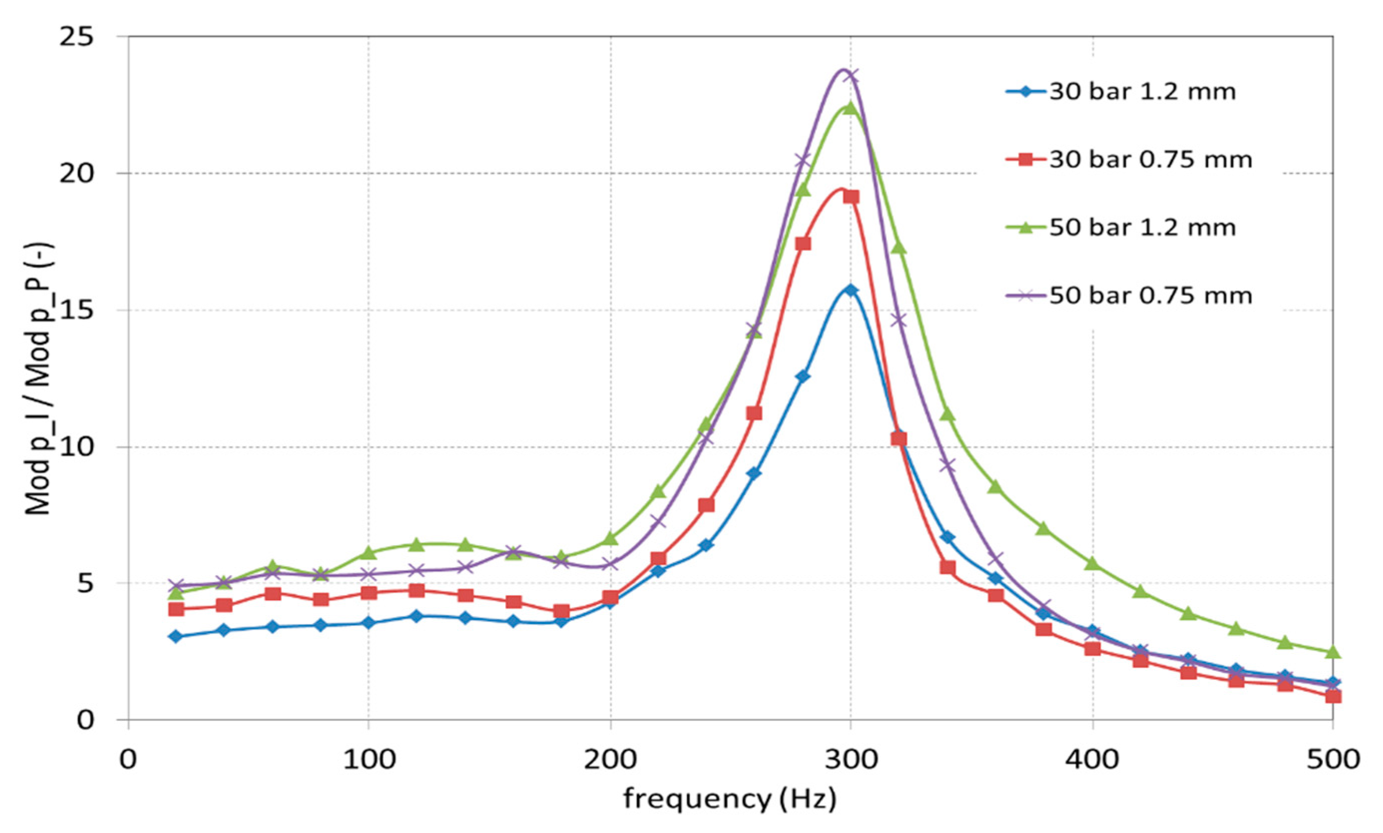
Starting from the amplitude of the first harmonic of both signals, the ratio between them was computed as a function of the frequency that was changed from 20 Hz to 500 Hz varying the pump speed:
In
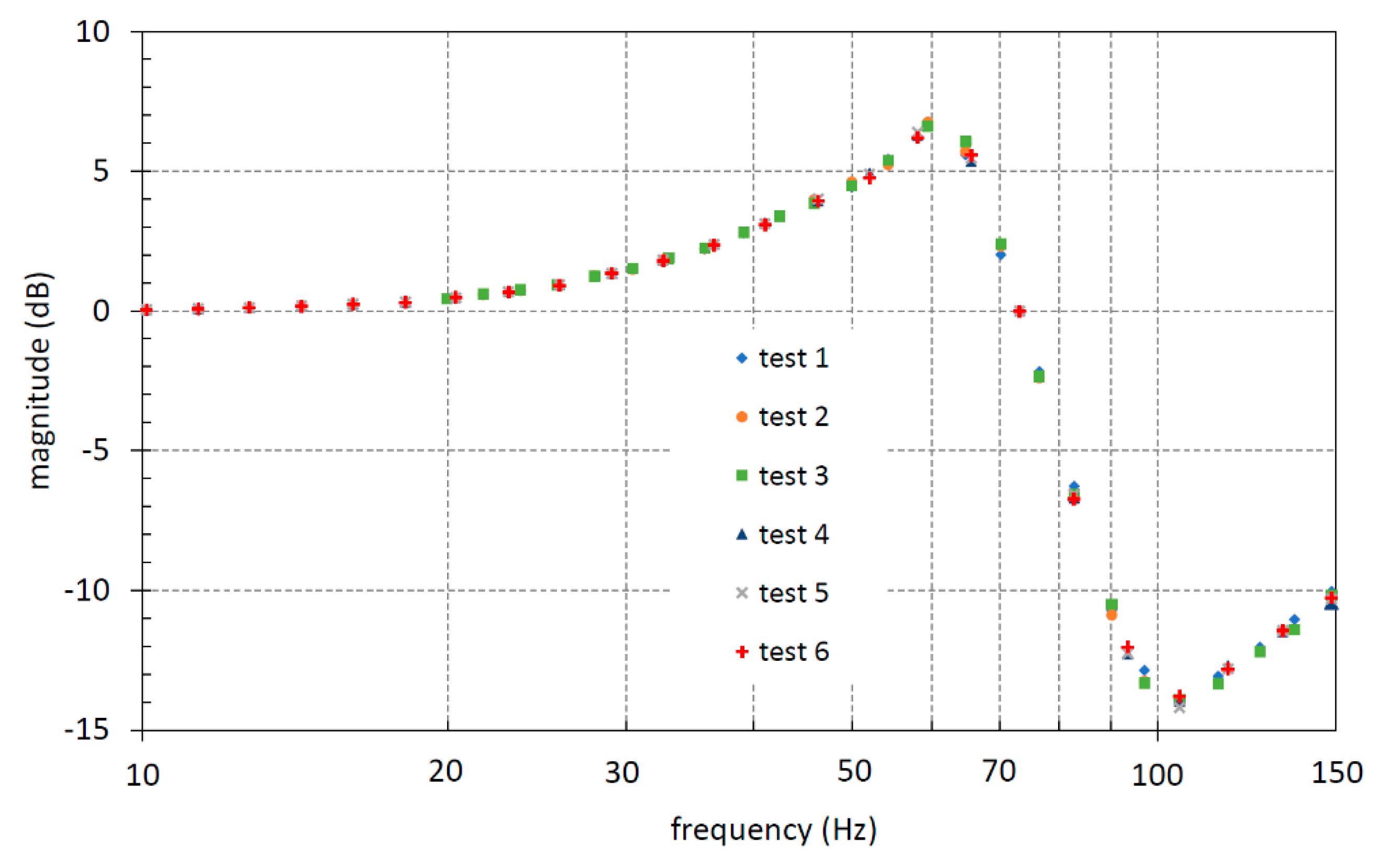
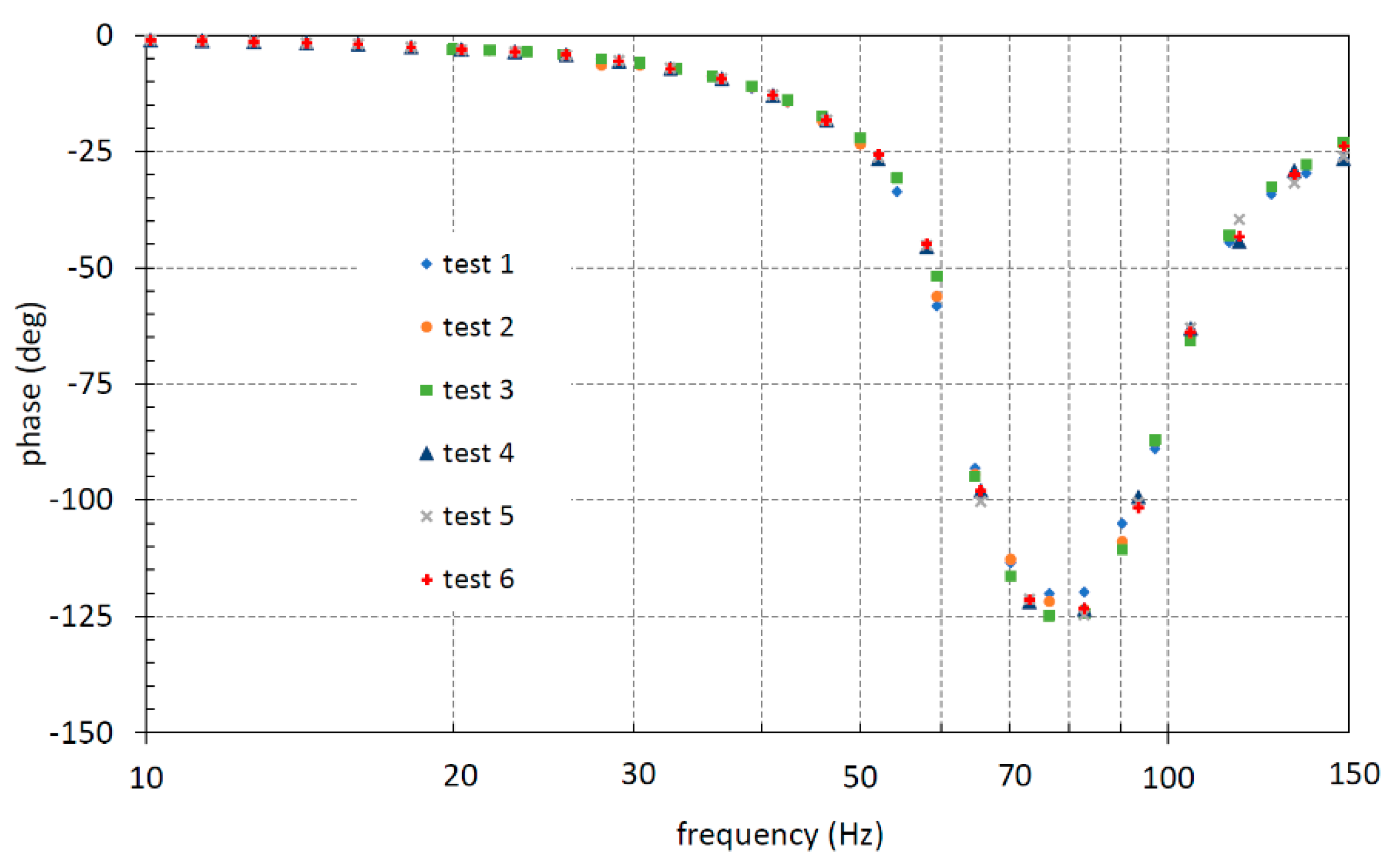
Figure 19 the Bode diagrams are reported with setting of the average inlet pressure at 30 and 50 bar and using an orifice with a diameter of 0.75 and 1.2 mm.
All Bode plots showed an underdamped system behavior, and the resonance frequency was always around 300 Hz in all the conditions investigated. This is a significant result because the resonance frequency can be theoretically calculated with Equation (19):
where k is the spring stiffness, and m is the total mass of the displaced components.
Evaluation of the Friction Coefficient
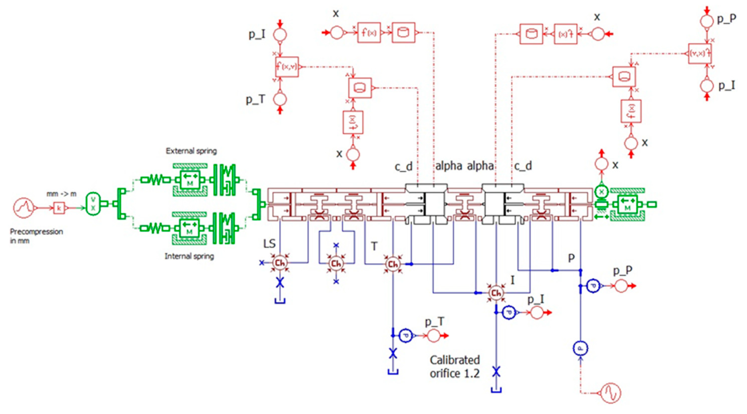
The target of this activity is to define the viscous friction coefficient. The mathematical model of the LS control was developed in the Amesim environment; the sketch is reported in
Figure 20.
The model calculates the instantaneous position and velocity of the spool using Newton’s second law; the force acting on the spool are due to fluid pressure, spring force, hydrodynamic force, and viscous friction force. The friction force is represented by the term
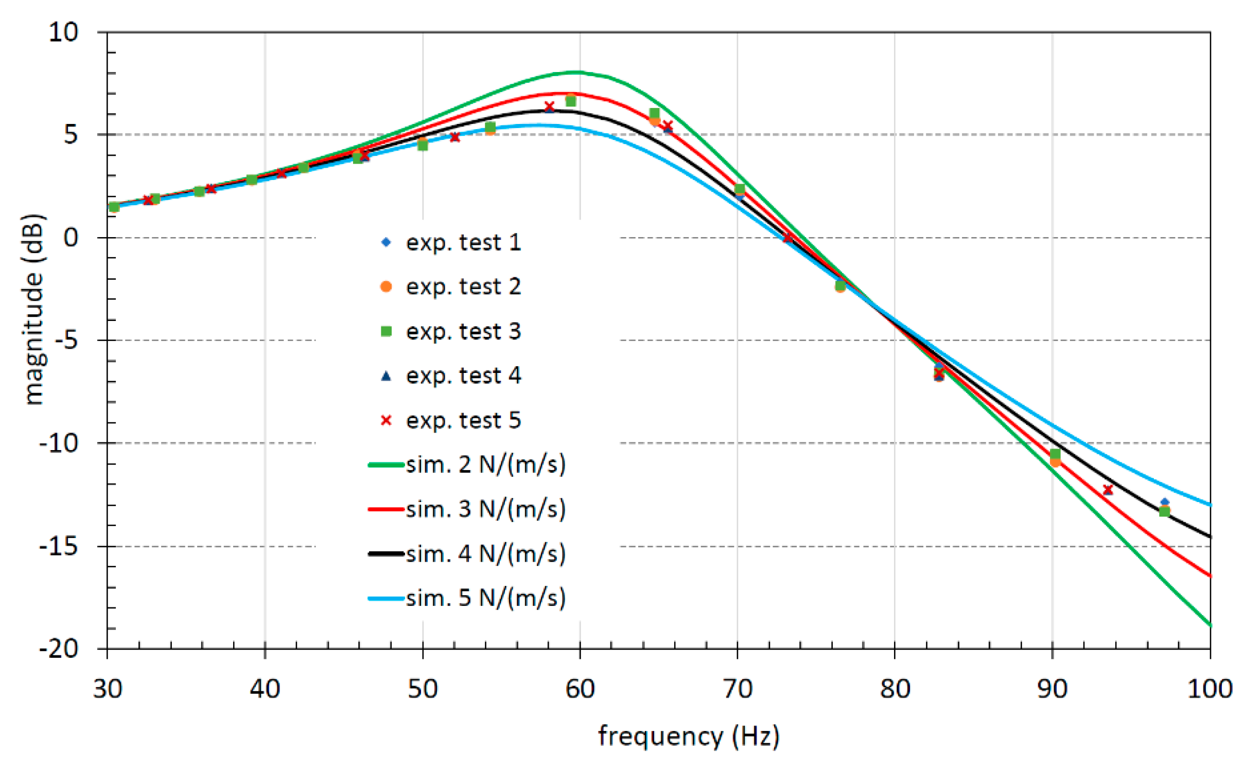
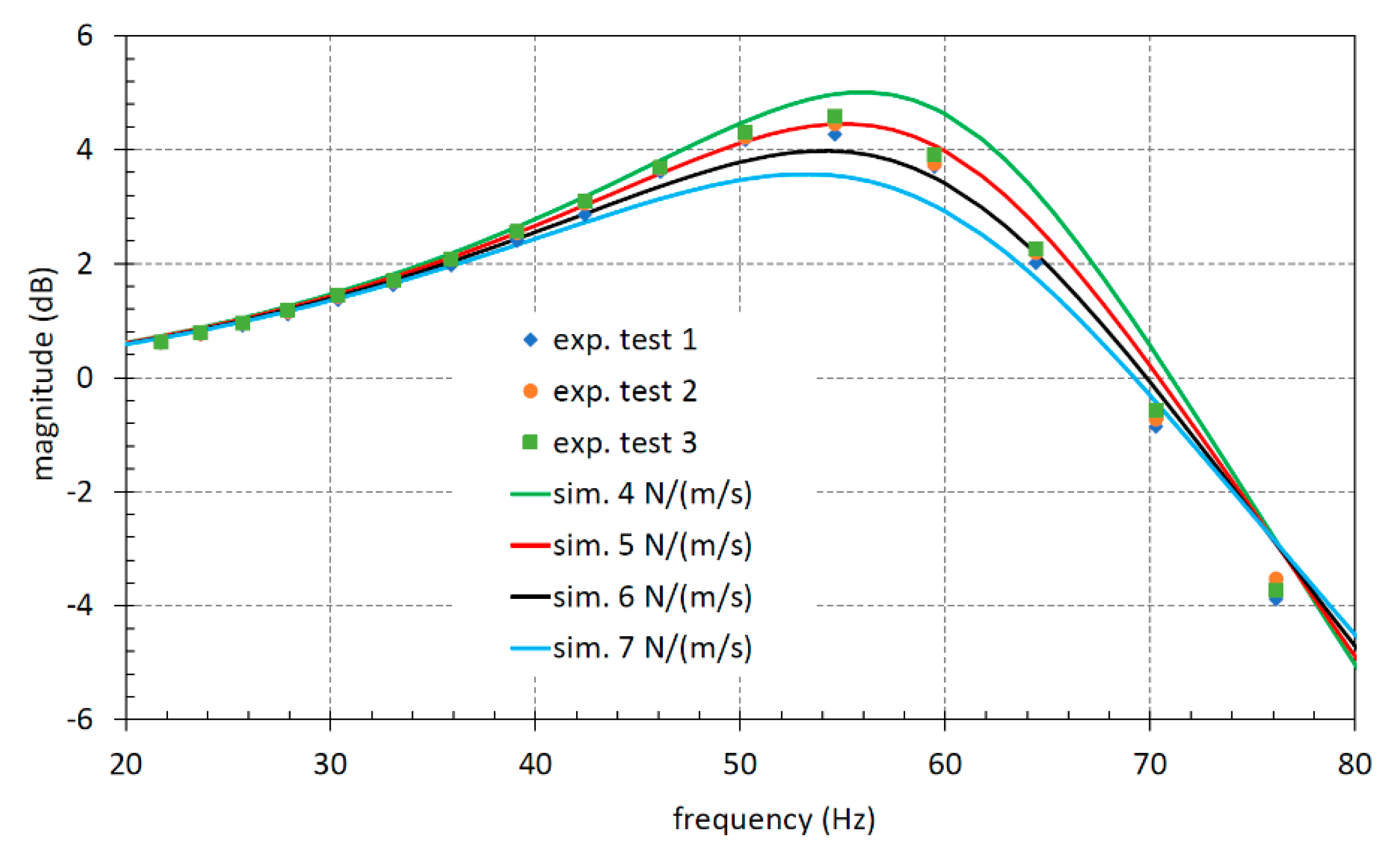
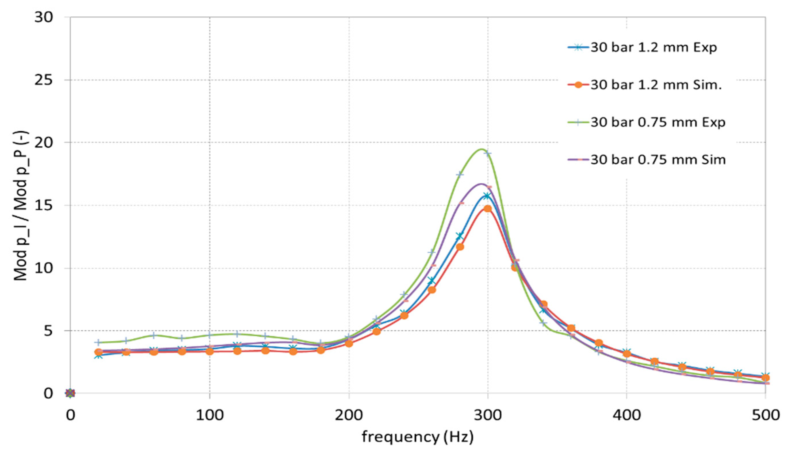
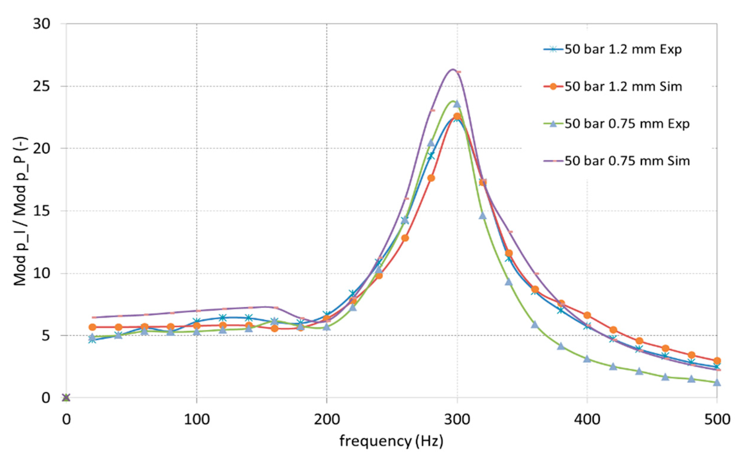
in Equation (4), where the coefficient c needs to be evaluated. To define this coefficient, several simulations were carried out by setting the pressure ripple acquired during the tests as input for the model and changing the value of the viscous friction coefficient to obtain a satisfactory agreement with the experimental data. The results presented in
Figure 21 and
Figure 22 show a satisfying agreement between numerical and experimental data. All these results were obtained by setting the viscous friction coefficient equal to 3.5 N/(m/s). It must be considered that the ratio of the pressures was also affected by other parameters, such as the discharge coefficient of the flow area. However, the underdamped system behavior and the resonance frequency were correctly estimated.
5. Discussion
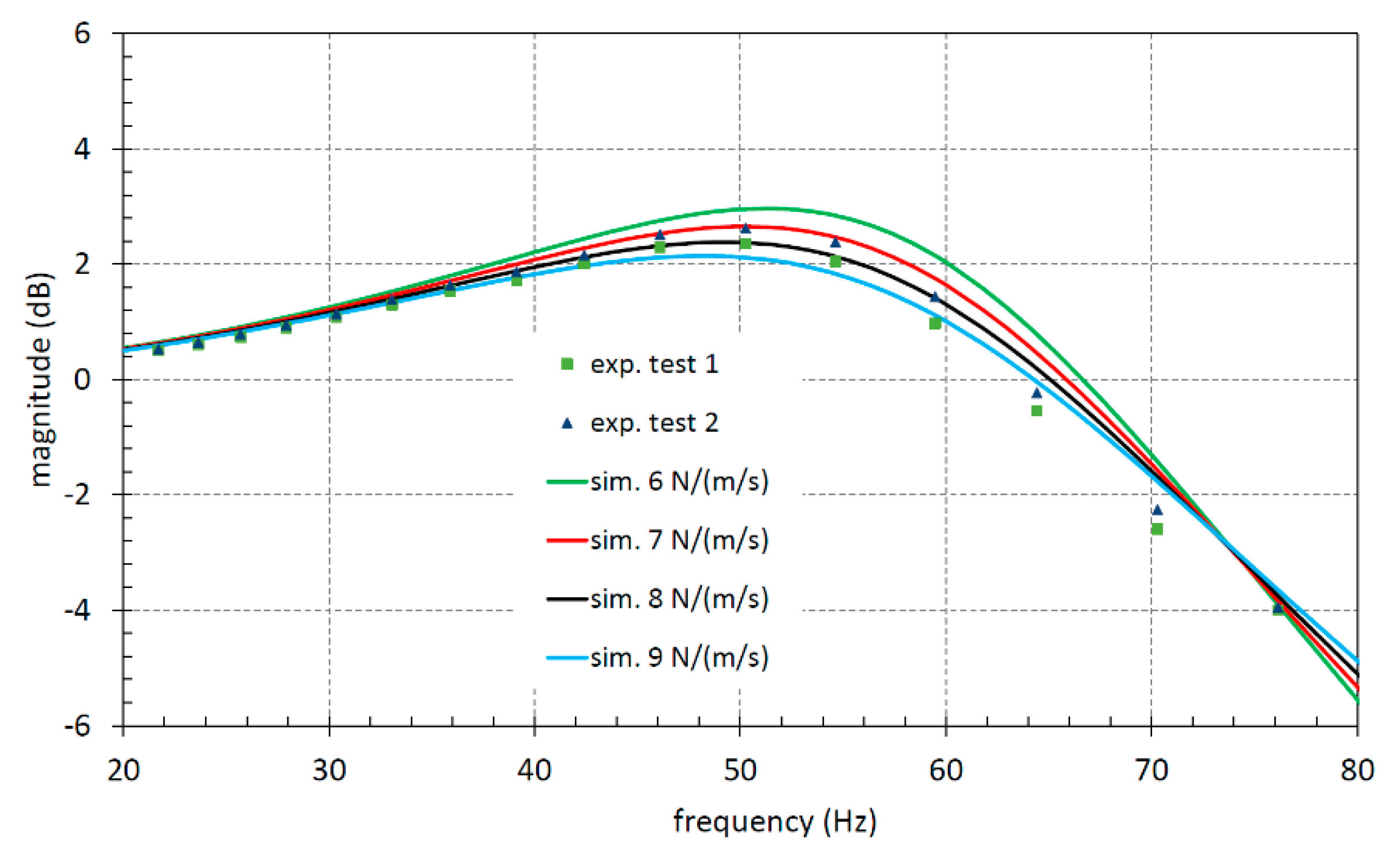
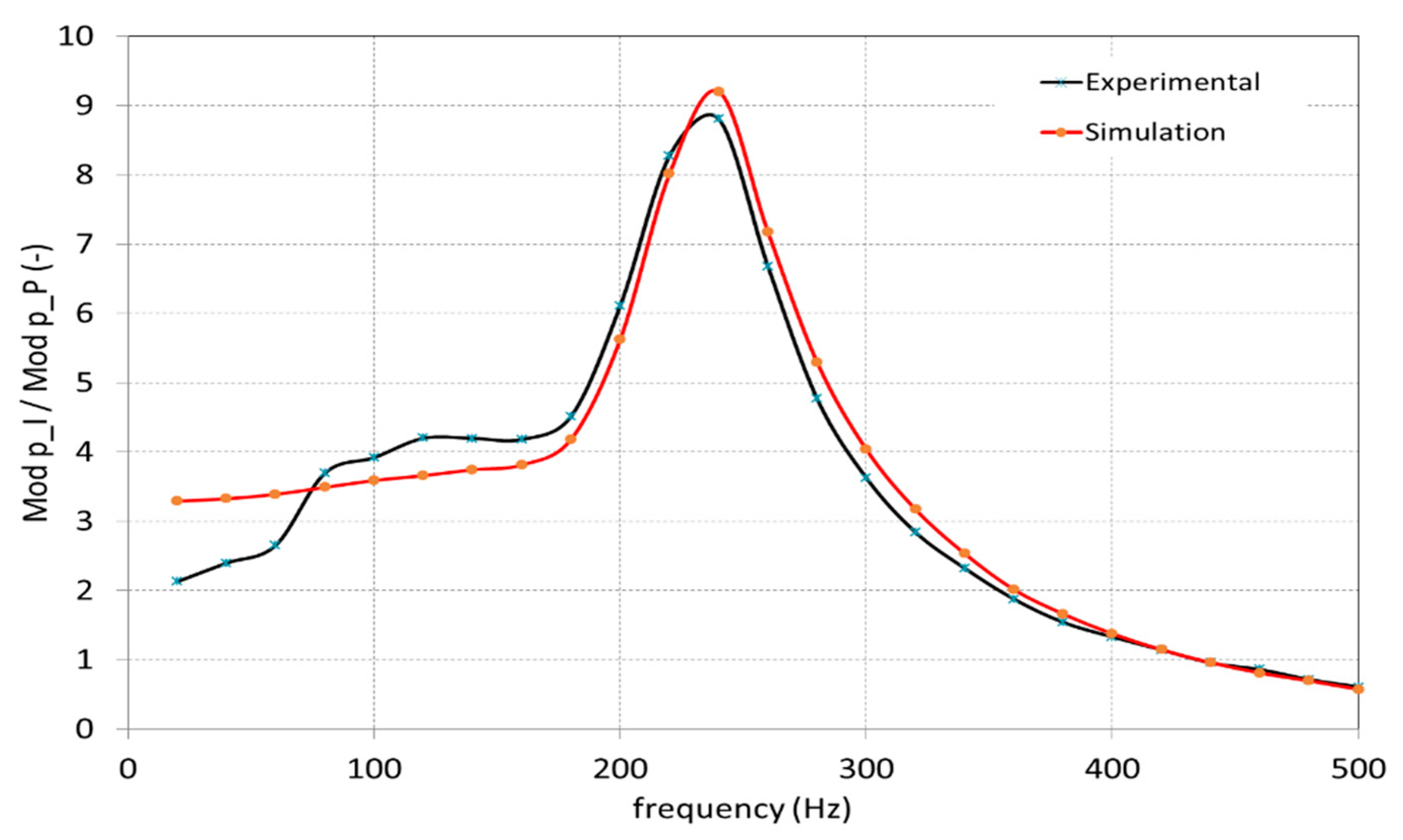
The methodologies presented are alternative ways for measuring the friction coefficient with respect to the installation of a displacement transducer that has the drawback of altering the displaced masses and friction losses. To analyze the effects of the presence of a linear variable displacement transducer (LVDT), further tests were carried out at the University of Parma.
Figure 23 reports the LVDT mounted on the component.
With this new configuration, the second method procedure was repeated, and the results obtained are reported in
Figure 24.
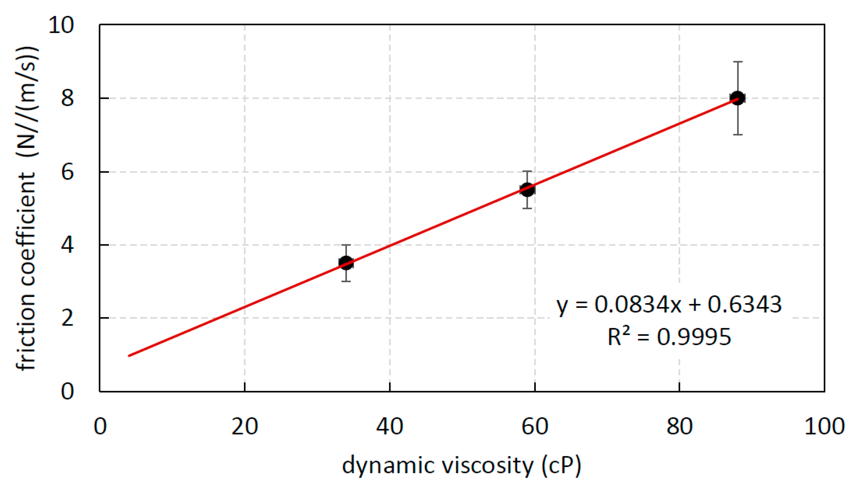
The resonance value was found at a lower value due to the increased mass of the displaced elements. With the theoretical formula a value of 237 Hz was found that, once again, is very similar to the resonance value shown in the diagrams. The mathematical model was able to reproduce the experimental outcomes by setting the friction coefficient equal to 7 N/(m/s), which is a significantly higher value with respect to what was found without the LVDT connected to the LS control spool. These latter results point out how a traditional approach based on the measurement of the spool displacement with an LVDT leads to an incorrect value of the friction coefficient.
Both presented methods lead to the same value of the viscous friction coefficient (3.5–4.0 N/(m/s)); then it is possible to say that the methods validate one each other. The first method is based on a rigorous mathematical description of the phenomenon that correlates the fluid pressure along the pipe; this method required a servovalve and a simultaneous acquisition of the pressures. The second method is mainly based on the experimental evidence, starting from the obvious correlation between the pressure oscillations at the outlet and the spool oscillations forced by a known inlet pressure ripple; this method has shown experimental results that firstly have reproduced the resonance frequency, which is easily calculable, and secondarily the dynamic behavior has been simulated setting a viscous friction coefficient with results equal to the value found with the first method.
The first method has the advantage that all parameters of the excitation pressure (frequency, mean value, amplitude, and even waveform) can be selected independently, while one of the strengths of the second method is that it is easier to generate quite high frequencies by means of the gear pump. As far as the complexity of the circuit layout is concerned, the first method does not require a circuit connected to all valve ports, since only the connection of the pipe is needed, while the advantage of the second is that the circuit for the generation of the flow rate is simpler.
The friction coefficient can be calculated with equations available in the literature [
18], equations that are often implemented in the main lumped parameter commercial simulation tools [
19,
20]. In [
18] the coefficient is calculated assuming a laminar gap with constant height h around the spool. Based on Newton’s law, the shear stress τ, defined as the ratio between the friction force F
f and the contact surface S, is given by Equation (20):
where v is the relative sliding velocity. Hence, the coefficient of proportionality between the force and the velocity is
However, if Equation (21) is applied for this valve, a value of c around 1 N/(m/s) is obtained. This value is much lower with respect to what found in this paper. A possible justification of this discrepancy can be the oversimplified hypothesis that considers the spool perfectly coaxial with respect to the housing. Since the clearance appears in the denominator, it is evident that any misalignment (eccentricity and tilt) can have a strong influence on the viscous friction coefficient. Hence, the value given by Equation (21) could represent a minimum value for the coefficient in ideal conditions.
Finally, the methodologies presented can be applied at different hydraulic components with similar coupling between sliding body and housing.


