An Uncertainty Assessment of Human Health Risk for Toxic Trace Elements Using a Sequential Indicator Simulation in Farmland Soils

Abstract

Toxic trace elements in farmland soils are potential threats to human health. In this study, we collected soil samples from the farmlands of southern Guangzhou. We used a sequential indicator simulation (SIS) to deal with the problem of skewed distribution in the sample data. We assessed the human health risks, as well as the uncertainties, of five toxic trace elements: arsenic (As), cadmium (Cd), chromium (Cr), lead (Pb), and mercury (Hg). The results were as follows: (1) The risk indices of two trace elements (Cd and Hg) were less than the standard threshold, which means that there was no human health risk due to Cd and Hg in the study area. However, the maximum risk indices of As, Cr, and Pb exceeded the standard threshold. In particular, the maximum risk index of Pb was twice the standard threshold; (2) The risk probabilities of As and Cr were less than 25% in most areas, and only a few parcels of farmland have a 100% risk probability. The risk map of Pb was used to identify contiguous areas of high-risk probability (i.e., 75%–100%) in the center of the study area. (3) E-type estimation by the SIS method overestimates the risk when the number of samples with concentrations above the threshold have a large proportion of total samples. Our conclusions are as follows: (1) The simulation results show that areas with high-risk indices were concentrated in the Panyu District, which is close to the Pearl River and the core urban area of Guangzhou; (2) Except for Pb, these trace elements are not likely to pose health risks in southern Guangzhou; (3) This study considers the risk probability found with the SIS method to be more reliable for visualizing regional risk.

1. Introduction

As a common land-use type, farmland affects human well-being [1]. However, with the rapid development of urbanization and industrialization, toxic trace elements may contaminate farmland soils through diverse ways, such as irrigation, deposition, and runoff [2]. Toxic trace elements in contaminated farmland can easily enter the human body through breathing, skin contact, and food intake [3], which can result in lesions or cancerous changes in the human body [4]. For example, cadmium (Cd) intake can cause diseases such as lung cancer, kidney dysfunction, and high blood pressure [5]. Lead (Pb) intake can cause symptoms such as lead poisoning, anemia, kidney disease, and gastrointestinal cramps [6]. Hexavalent chromium (Cr) is a recognized carcinogen [7]. The body’s central nervous system is affected negatively by arsenic (As) and mercury (Hg) intake [8,9]. The long-term accumulation of toxic trace elements in farmland comprises a major threat to human health. Regional health risk status of toxic trace elements are important for the protection of human health, food security, and farmland environments [10]. In order to obtain regional health risks accurately and effectively, it is important to quantify trace element toxicity [11]. Human health risk assessment is a key method for risk quantification [12,13], which can help in the management of health risks, pollution warnings, and soil restoration [14].

Human health risk assessment calculates the risk of toxic trace elements by using the elemental concentrations of the samples [11,15]. There are two types of methods for human health risk assessment: methods based on deterministic models and methods based on stochastic models.

The first type of method is based on deterministic models. These methods construct a risk assessment model using the mechanisms of the exposure pathway, dose-response relationship, and crop reflection relationship. This type of model obtains the required parameters by referring to relevant institutional guidelines or scholarly research. Then, the health risk of the study area is calculated by the average hazard index with the soil trace element concentrations at the sampling points [16,17]. For example, Gu et al. [18] referred to the manual exposure factors and parameters in the technical guidelines for contaminated site risk assessment [19], in order to obtain human health risk assessments in 28 urban parks in Guangzhou. They calculated the average hazard index of the carcinogenic and non-carcinogenic risk of each park and concluded that no human health risk existed in the urban parks in Guangzhou. Sawut et al. [7] used a series of existing studies to determine the intake rate, intake time, and other parameters of trace elements. They calculated average hazard indices for both children and adults, and obtained the human health risks of vegetables in Northwest China. However, due to the individual differences of soil environmental variables and a lack of prior knowledge, trace element concentrations may have a high degree of spatial variability. The parameters of this model, therefore, have considerable uncertainty. Most of these parameters are determined directly by referring to existing guidelines or research. Moreover, the researchers calculated the average value of the hazard index to obtain the degree of regional risk, which may lead to smoothing effects. This method might overestimate or underestimate the risk. Some researchers have estimated the regional risk without considering the uncertainties involved [20].

The second type of method is based on stochastic models. These methods use stochastic simulation to calculate the uncertainty of the model parameters for human health risk assessment [21,22]. The stochastic simulation takes values randomly based on the cumulative distribution of the variable data, and produces multiple simulation results to obtain the risk and its uncertainty [23]. For example, Chen et al. [20] used a Monte Carlo simulation to solve the parameter uncertainty problem caused by a lack of prior knowledge when evaluating human health risk in the surface soil of Beijing. They obtained the human health risk situation and its uncertainty in the Beijing sampling area. Albuquerque et al. [24] used a sequential Gaussian simulation to obtain the uncertainty of the high and low-risk areas while studying the risk levels of 14 trace elements in the Aviles Estuary in Spain, and visualized the risk using a mean value map. However, data conforming to a normal distribution is a requirement for these methods. For instance, a Monte Carlo simulation may lead to more errors when the number of samples is not sufficient or the probability distribution is biased. In addition, a sequential Gaussian simulation loses information when the data are processed and transformed.

Human health risk assessment based on the uncertainty model can objectively reflect the risk of toxic trace elements. However, the current uncertainty model research is based on the condition that the frequency distribution of the sample data follow a normal distribution. Meeting the normal distribution requirements may be difficult when using sample data of trace elements in farmland, especially when the trace element concentrations have abnormal values. Simple abnormal value processing methods are prone to smoothing effects, which results in the loss of information in key areas [14,25]. Moreover, due to the cost limitations of sampling, the number of samples is often limited. Abnormal values influence the frequency distribution, but often contain information about contamination by toxic trace elements. Therefore, we cannot simply eliminate the abnormal values. Therefore, we need to study the use of uncertainty models in obtaining human health risk when the frequency distribution of the sample data has a non-normal distribution.

To obtain the human health risk of toxic trace elements in farmland, this study uses a non-parametric statistical sequential indicator simulation method to address the problem of the sample data frequency distribution. This study focuses on (1) simulating the regional farmland health risk of each trace element; (2) assessing their uncertainty; and (3) mapping the spatial distribution of the human health risk probability.

2. Materials and Methods

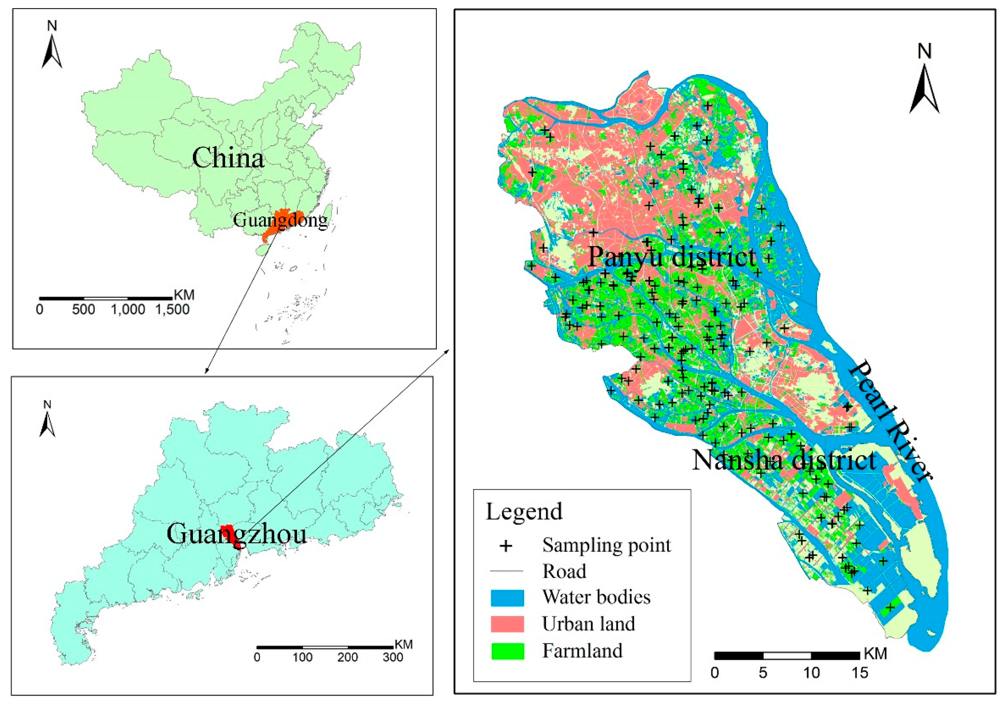
2.1. Study Area

The accumulation of toxic trace elements in farmland, especially around megacities, may result in a high probability of human health risks [18,20]. Guangzhou, a rapidly growing city, is one of the largest cities in South China. Guangzhou is located in the center of Guangdong Province, and is adjacent to Hong Kong and Macau. Guangzhou has a maritime subtropical monsoon climate, with an annual average temperature of 22.8 °C and average annual precipitation of 1800 mm. The Pearl River system passes through Guangzhou. It has a population of over 20 million. Human activity has a huge impact on this city. Due to the high degree of urbanization, few farmlands remain in the main urban areas of Guangzhou. Therefore, we selected the southern part of Guangzhou (i.e., Panyu and Nansha District) as the study area in this study, which has a lower urbanization level and contiguous farmland.

2.2. Soil Sampling and Laboratory Analysis

We designed the sampling plan according to land use/cover data of the study area. We sampled in the farmland as evenly as possible, with 195 samples (0–20 cm) throughout the farmland in 2015. Figure 1 shows the spatial distribution of the sample points.

In this study, the selection of trace elements was based on the existing toxic trace element contamination research of Guangzhou [26,27,28]; we also refer to the “12th Five-Year Plan for Heavy Metals Contamination Comprehensive Prevention and Control” of China, and the “13th Five-Year Plan for Heavy Metals Contamination Comprehensive Prevention and Control” of Guangdong Province. We selected five trace elements for study: lead (Pb), cadmium (Cd), chromium (Cr), mercury (Hg), and arsenic (As). We determined the total amounts of these five trace elements. We used the HF-HNO₃-HClO₄ digestion method to process lead (Pb), cadmium (Cd), and chromium (Cr). We determined Cd and Pb by graphite furnace atomic absorption spectrometry and we determined Cr by flame atomic absorption spectrophotometry. The atomic absorption spectrometer (graphite furnace) used was the Z-2000 (HITACHI). The flame atomic absorption spectrometer used was the Z-5300 (HITACHI). Arsenic (As) and mercury (Hg) were processed with HCl-HNO₃ and were determined by reduction-gasification atomic fluorometry. The atomic fluorescence photometer used was the AFS-930 double-pipe atomic fluorescence spectrometer (Beijing Titan Instruments).

2.3. Uncertainty Assessment of Human Health Risks

2.3.1. Sequential Indicator Simulation of Soil Data

Sequential indicator simulation is a stochastic simulation method based on non-parametric statistics. Its indicator model has good flexibility and does not require the data used to satisfy any certain distribution type [29,30,31]. Moreover, the simulation has a small smoothing effect. This method does not ignore abnormal values in areas, which makes the simulation result closer to the real situation [14]. Information about the extreme values in the abnormal region can be utilized [32].According to the existing research, SIS can be divided into the following four steps [29]:

(1) The original sampled data are indicator transformed. The user obtains a priori conditional cumulative distribution function (CCDF) according to the Kriging method. $\left\{Z\left(x_i\right),i=1,2,\dots ,n\right\}$ is a set of sampled data under the K-group threshold (${\mathrm{z}}_{\mathrm{k}}$). The more quantiles (thresholds) that are selected, the more reliable the CCDF is [33]. The indicator variables are encoded as 0 or 1 by the indicator function $\mathrm{I}\left({\mathrm{x}}_{\mathrm{i}}\right)$ (Equation (1)) [29]:

$$\mathrm{I}({\mathrm{x}}_{\mathrm{i}})=\{\begin{array}{c}1, \mathrm{x}\le {\mathrm{z}}_{\mathrm{k}}\\ 0, \mathrm{x}>{\mathrm{z}}_{\mathrm{k}}\end{array}\hspace{1em}\left(\mathrm{k}=1,2,\dots ,K\right).$$

(1)

(2) Using the known raw data as conditional data, the user obtains the conditional prior probability $\mathrm{F}\left(x\right)=Z\left(x_i\right)\le z_k\left|C\right(x_i)$. This probability uses the indicator Kriging estimate to extrapolate its conditional cumulative distribution function F_z(x).

(3) The user divides the study area into grids of uniform resolution and defines a random path through all grid nodes. This method extracts a value from F_z(x) randomly as the simulation value at the first grid position. Then, the user obtains the estimated value $\hat{I}$ of the CCDF at the target grid (Equations (2)) [29]:

$$\hat{I}(x_0;z_k)={\mathrm{Prob}}^{\ast }\left(Z\left(x_i\right)\le z_k\left|C\right(x_i)\right).$$

(2)

(4) The above new value is added to the conditional data set. The grid’s prior condition cumulative distribution function F_z(x) for the next simulation position is modeled by this new data set. This process is repeated until all grid nodes are simulated.

This method obtains n realizations by repeating the above-mentioned steps. In n realizations, the number of grid values exceeding the threshold is n₁ and the uncertainty (above threshold probability) of this grid is n₁/n. Each realization of the sequential indicator simulation has equal probability [25,32]. Some studies have also used conditional means (E-type estimate) of n realizations to obtain the spatial distribution of trace element concentrations [29,30,31]. In the calculation process, we used the GS + 9.0 software to obtain the experimental semivariogram and variogram models of each threshold. We realized the stochastic simulation with the SGeMS v2.5b software.

2.3.2. Human Health Risk Assessment

Human health risks contain carcinogenic and non-carcinogenic risks. Toxic trace elements enter into the human body in different ways, such as oral intake, skin contact, and inhalation [34]. Existing research has demonstrated that As and Cd have carcinogenic effects [35]. Hexavalent chromium (Cr⁶⁺) is carcinogenic to humans, but trivalent chromium (Cr³⁺) has not been defined as being carcinogenic yet [35]. However, Cr⁶⁺ is more unstable than Cr³⁺ in nature [36]. Chromium in the soil is more inclined towards the stable state of Cr³⁺ [37]. Therefore, the reference parameter is the parameter of Cr³⁺ in this study, and we only consider the non-carcinogenic risk of Cr. The non-carcinogenic assessment of trace elements include Hg, Pb, and Cr. We used an exposure model based on the US EPA model [38]. The equations (

Table A1. Equations of each parameter.

Parameter	Type	Equation
Carcinogenic exposure value	Oral	$OISE{R}_{ca}=\left(OISE{R}_c\times E{D}_c\times E{F}_c/B{W}_c+OISE{R}_a\times E{D}_a\times E{F}_a/B{W}_a\right)\times AB{S}_o\times {10}^{-6}$
	Dermal	$DCSE{R}_{ca}=(SA{E}_c\times SSA{R}_c\times E{F}_c\times E{D}_c\times E_V/B{W}_c+SA{E}_a\times SSA{R}_a\times E{F}_{ca}\times E{D}_a\times E_V/B{W}_a)\times AB{S}_d/A{T}_{ca}\times {10}^{-6}$
	Inhalational	$PISE{R}_{ca}=P{M}_{10}\times DAI{R}_c\times E{D}_c\times PIAF\times \left(fspo\times EF{O}_c+fspi\times EF{I}_c\right)/\left(B{W}_c\times A{T}_{ca}\right)\times {10}^{-6}+P{M}_{10}\times DAI{R}_a\times E{D}_a\times PIAF\times \left(fspo\times EF{O}_a+fspi\times EF{I}_{ca}\right)/B{W}_a\times A{T}_{ca}\times {10}^{-6}$
Non-carcinogenic exposure value	Oral intake	$OISE{R}_{nc}=OISE{R}_c\times E{D}_c\times E{F}_c\times AB{S}_o/B{W}_c\times A{T}_{nc}\times {10}^{-6}$
	Dermal	$DCSE{R}_{nc}=SA{E}_c\times SSA{R}_c\times E{F}_c\times E{D}_c\times E_V\times AB{S}_d/B{W}_c\times A{T}_{nc}\times {10}^{-6}$
	Inhalational	$PISE{R}_{nc}=P{M}_{10}\times DAI{R}_c\times E{D}_c\times PIAF\times \left(fspo\times EF{O}_c+fspi\times EF{I}_c\right) /B{W}_c\times A{T}_{nc}\times {10}^{-6}$

Note: $OISER$ means oral ingestion of soil exposure.$DCSER$ means soil exposure through skin contact routes. $PISER$ means soil exposure to inhaled particulate matter.

) and parameters (

Table A2. Values of each parameter.

Parameter	Symbol	Units	Value	Reference
Exposure duration of children	EDc	a	6	(MEPPRC, 2014)a
Exposure duration of adults	EDa	a	24	(MEPPRC, 2014)a
Exposure frequency of children	Efc	d·a−1	350	(MEPPRC, 2014)a
Exposure frequency of adults	Efa	d·a−1	350	(MEPPRC, 2014)a
Average body weight of children	BWc	kg	56.8	(MEPPRC, 2014)a
Average body weight of adults	Bwa	kg	15.9	(MEPPRC, 2014)a
Absorption factor of oral ingestion	ABSo	unitless	1	(MEPPRC, 2014)a
Average time for carcinogenic effect	ATca	d	26,280	(MEPPRC, 2014)a
Average time for non-carcinogenic effect	Atnc	d	2190	(MEPPRC, 2014)a
Exposed skin surface area of adults	SAEa	cm2	5074.89	(MEPPRC, 2014)a
Exposed skin surface area of children	SAEc	cm2	2447.56	(MEPPRC, 2014)a
Adherence rate of soil on skin for adults	SSARa	mg·cm−2	0.07	(MEPPRC, 2014)a
Adherence rate of soil on skin for children	SSARc	mg·cm−2	0.2	(MEPPRC, 2014)a
Daily exposure frequency of dermal contact event	Ev	times/d	1	(MEPPRC, 2014)a
Content of inhalable particulates in ambient air	PM10	mg·m−3	0.15	(MEPPRC, 2014)a
Daily air inhalation rate of adults	DAIRa	m3·d−1	14.5	(MEPPRC, 2014)a
Daily air inhalation rate of children	DAIRc	m3·d−1	7.5	(MEPPRC, 2014)a
Retention fraction of inhaled particulates in body	PIAF	unitless	0.75	(MEPPRC, 2014)a
Fraction of soil-borne particulates in indoor air	fspi	unitless	0.8	(MEPPRC, 2014)a
Fraction of soil-borne particulates in outdoor air	fspo	unitless	0.5	(MEPPRC, 2014)a
Indoor exposure frequency of adults	EFIa	d·a−1	262.5	(MEPPRC, 2014)a
Indoor exposure frequency of children	EFIc	d·a−1	262.5	(MEPPRC, 2014)a
Outdoor exposure frequency of adults	EFOa	d·a−1	87.5	(MEPPRC, 2014)a
Outdoor exposure frequency of children	EFOc	d·a−1	87.5	(MEPPRC, 2014)a
Soil allocation factor	SAF	unitless	0.2	(MEPPRC, 2014)a
Dermal absorption factor of Cd	ABSDCd	unitless	0.001	(USEPA, 2013)b
Dermal absorption factor of CR	ABSDCr	unitless	0.001	(USEPA, 2013)b
Dermal absorption factor of As	ABSDAs	unitless	0.03	(USEPA, 2013)b
Dermal absorption factor of Hg	ABSDHg	unitless	0.05	(HC, 2004)c
Dermal absorption factor of Pb	ABSDPb	unitless	0.006	(HC, 2004)c

^a Chinese MEP. (2014). Technical guidelines for risk assessment of contaminated sites (HJ25.3-2014, published in Chinese). China Environmental Science Press Beijing. ^b USEPA. (2013). Regional Screening Levels (RSL) for Chemical Contaminants at Superfund Sites. Washington DC: USEPA. ^c Health Canada. (2004). Federal Contaminated Site Risk Assessment in Canada-Part II: Health Canada Toxicological Reference Values (TRVs) and Chemical-Specific Factors. Ottawa.

and

Table A3. Parameters for each trace element toxicity.

Parameter		SFo (mg/kg-day)	SFd (mg/kg-day)	SFi (mg/kg-day)	RfDo (mg/kg-day)	RfDd (mg/kg-day)	RfDi (mg/kg-day)
Carcinogenic Elements	As	1.50	1.50	16.84	-	-	-
	Cd	3.80 × 10−1	2.00	329.05	-	-	-
Non-carcinogenic elements	Hg	-	-	-	3.00 × 10−4	2.10 × 10−5	7.66 × 10−5
	Pb	-	-	-	3.50 × 10−4	5.25 × 10−4	3.52 × 10−2
	Cr	-	-	-	1.50	1.95 × 10−2	2.55 × 10−5

Note: SFo means oral intake carcinogenic slope factor. SFd means skin contact carcinogenic slope factor. SFi means inhalation carcinogenic slope factor. RfDo means oral intake reference dose. RfDd means skin contact reference dose. RfDi means inhalation reference dose.

) refer to the Technical Guidelines For Risk Assessment of Contaminated Sites and Regional Screening Levels [19,38]. Due to the different dietary and living habits of people in different countries, the exposure parameters of health risk are different. The Technical Guidelines For Risk Assessment of Contaminated Sites was used to correct some parameters, according to the actual situation in China [19].

This study takes into account the effects of toxic trace elements on adults and children. The tolerance value for carcinogenic risk (CR) is < 10⁻⁴ [19,38]. A non-carcinogenic hazard index (HI) below 1.0 indicates the absence of non-carcinogenic health risk [19,38]. We used the ArcGIS 10.2 software to visualize the risk. The risk assessment model (Equations (3)–(10)) was as follows [19,38]:

(1) Carcinogenic:

$$\mathrm{Oral} \mathrm{risk}: C{R}_{ois}=OISE{R}_{ca}\times C_{sur}\times S{F}_o$$

(3)

$$\mathrm{Dermal} \mathrm{risk}: C{R}_{dcs}=DCSE{R}_{ca}\times C_{sur}\times S{F}_d$$

(4)

$$\mathrm{Inhalational} \mathrm{risk}: C{R}_{pis}=PISE{R}_{ca}\times C_{sur}\times S{F}_i$$

(5)

$$\mathrm{Carcinogenic} \mathrm{risk}: C{R}_n=C{R}_{ois}+C{R}_{dcs}+C{R}_{pis}$$

(6)

(2) Non-carcinogenic:

$$\mathrm{Oral} \mathrm{risk}: \mathit{H}{\mathit{Q}}_{\mathit{o}\mathit{i}\mathit{s}}=\mathit{O}\mathit{I}\mathit{S}\mathit{E}{\mathit{R}}_{\mathit{n}\mathit{c}}\times {\mathit{C}}_{\mathit{s}\mathit{u}\mathit{r}}/\left(\mathit{R}\mathit{f}{\mathit{D}}_{\mathit{o}}\times \mathit{S}\mathit{A}\mathit{F}\right)$$

(7)

$$\mathrm{Dermal} \mathrm{risk}: \mathit{H}{\mathit{Q}}_{\mathit{d}\mathit{c}\mathit{s}}=\mathit{D}\mathit{C}\mathit{S}\mathit{E}{\mathit{R}}_{\mathit{n}\mathit{c}}\times {\mathit{C}}_{\mathit{s}\mathit{u}\mathit{r}}/\left(\mathit{R}\mathit{f}{\mathit{D}}_{\mathit{d}}\times \mathit{S}\mathit{A}\mathit{F}\right)$$

(8)

$$\mathrm{Inhalational} \mathrm{risk}: \mathit{H}{\mathit{Q}}_{\mathit{p}\mathit{i}\mathit{s}}=\mathit{P}\mathit{I}\mathit{S}\mathit{E}{\mathit{R}}_{\mathit{n}\mathit{c}}\times {\mathit{C}}_{\mathit{s}\mathit{u}\mathit{r}}/\left(\mathit{R}\mathit{f}{\mathit{D}}_{\mathit{i}}\times \mathit{S}\mathit{A}\mathit{F}\right)$$

(9)

$$\mathrm{Non}-\mathrm{carcinogenic} \mathrm{risk}: \mathit{H}{\mathit{I}}_{\mathit{n}}=\mathit{H}{\mathit{Q}}_{\mathit{o}\mathit{i}\mathit{s}}+\mathit{H}{\mathit{Q}}_{\mathit{d}\mathit{c}\mathit{s}}+\mathit{H}{\mathit{Q}}_{\mathit{p}\mathit{i}\mathit{s}}.$$

(10)

2.3.3. Uncertainty Model Accuracy Evaluation

The accuracy of the uncertainty model was evaluated by the symmetric p-probability intervals (p-PI) [29]. The conditional cumulative probability distribution function $F\left(u;\zeta \right)$ at any location u allows for the computation of p-PI bounded by (1-p)/2 and (1+p)/2. For example, the 0.5-PI representation is $[F^{-1}\left(u;0.25\right),F^{-1}\left(u;0.75\right)]$. In this case, the correct uncertainty model would show that there is a 0.5 probability that the actual observations at u falls into this interval [29]. We calculated the probability that an observation falls into p-PIs as follows (Equations (11) and (12)) [29]:

$$\overline{\zeta }\left(p\right)=1/N\times {{\displaystyle \sum }}_{j=1}^N\zeta (u_j;p),\hspace{1em}\left(j=1,\dots ,N;N=195\right).$$

(11)

$$\mathsf{\zeta }\left(u_j;p\right)=\{\begin{array}{c}1\hspace{1em}if F^{-1}\left(u_j;\left(1-p\right)/2\right)<Z\left(u_j\right)<F^{-1}\left(u_j;\left(1+p\right)/2\right)\\ 0\hspace{1em}\hspace{1em}\hspace{1em}\hspace{1em}\hspace{1em}\hspace{1em}\hspace{1em}\hspace{1em}otherwise\end{array}.$$

(12)

A smaller root mean square error (RMSE) means higher accuracy [39]. The RMSE was calculated as follows (Equation (13)) [39]:

$$RMSE=\sqrt{\mathbf{1}/\mathit{n}\times {{\displaystyle \sum }}_{\mathit{i}=\mathbf{1}}^{\mathit{n}}{\left[{\mathit{p}}_{\mathit{i}}-\overline{\mathit{\zeta }}\left(\mathit{p}\right)\right]}^{\mathbf{2}}\hspace{1em}}\left(\mathit{i}=\mathbf{1},\dots ,\mathit{n};\mathit{n}=\mathbf{195}\right).$$

(13)

3. Results and Discussion

3.1. Preliminary Data Description

Table 1. General descriptive statistics of each trace element.

Element	Mean (mg/kg)	Minimum (mg/kg)	Maximum (mg/kg)	Standard Deviation (mg/kg)	Skewness	Kurtosis	Coefficient of Variation	Background Value (mg/kg)	Kolmogorov-Smirnov Significance
Cd	0.18	0.05	0.48	0.06	0.58	1.53	36%	0.11	3.60 × 10−1
Hg	0.13	0.03	0.46	0.08	1.59	2.02	63%	0.13	0
As	10.30	0.66	42.62	8.34	1.67	2.89	81%	25	8.28 × 10−5
Pb	51.75	19.10	122.00	16.48	1.47	3.87	32%	60	1.39 × 10−2
Cr	69.74	20.83	156.47	22.63	0.22	0.23	32%	77	3.57 × 10−1

Note: Kolmogorov Smirnov significance less than 0.05 means that the data do not meet the normal distribution.

shows the results of the descriptive statistics of five trace elements in southern Guangzhou farmland.

The main soil types of farmland were paddy soils and red soils in study area. The main soil texture was loam. The clay content was in the range of 22%–43%. The maximum, average, and minimum pH values were 8.2, 5.7, and 3.9, respectively. By comparing the background values of risk screening values for soil trace elements of the Pearl River Delta area [40], the maximum values of the five trace elements were seen to be higher than the soil background values. This indicated that trace elements have external inputs in the study area. Furthermore, the average values for Cd and Hg were larger than the soil background values, indicating that the Cd and Hg accumulation was high. Previous studies have found that urban land and mining areas had contamination of toxic trace elements in Guangzhou [18]. Soil trace elements of farmland in Guangzhou are likely to pose risks to crops, humans, and the environment. Due to the high urbanization development in Guangzhou, as seen in Figure 1, farmland in the Panyu and Nansha Districts is very close to urban areas. Therefore, studies of the human health risks of toxic trace elements in this farmland has been deemed necessary.

The coefficient of variation (CV) is the ratio of the standard deviation to the mean [41]. The CV reflects the degree of dispersion of variables. The coefficient of variation of the five trace elements was in the range of 32%–81%. The order of variation was As > Hg > Cd > Cr = Pb. The coefficients of variation of As and Hg were relatively large, indicating that these two trace elements may be greatly affected by human activity. The asymmetry coefficients (skewness) of the five trace elements were all greater than 0, as can be seen in Table 1; therefore, their data frequency distributions had a certain positive bias. The order of deviation was As > Hg > Pb > Cd > Cr. The Kolmogorov-Smirnov (K-S) test showed that As and Hg had a significance of less than 0.05, which means that their data distribution was not normal. We could not use those data to provide a good result with some uncertainty models, such as Monte Carlo or a sequential Gaussian simulation [42].

3.2. Uncertainty Assessment of Human Health Risk Based on SIS

3.2.1. Human health Risk Threshold of Each Trace Element

We used the concentrations of trace elements to calculate human health risks at each sample point. Then, we calculated the average values of sample points to obtain the human health risk indices (CR or HI) for the five trace elements. According to the risk standard value, a cancer risk index (CR) below 10⁻⁴ is acceptable, and the non-carcinogenic hazard index (HI) indicates no hazard when it has a value less than 1.0. As shown in

Table 2. The cancer risk index (CR), non-carcinogenic hazard index (HI), and threshold of human health risk of each trace element.

	Carcinogenic Elements		Non-Carcinogenic Elements
	As	Cd	Hg	Pb	Cr
CR (Mean)	2.80 × 10−5	6.94 × 10−7	-	-	-
HI (Mean)	-	-	0.07	0.98	0.51
Threshold (mg/kg)	36.81	26.27	1.80	52.85	137.34

, the CR of As and Cd were less than 10⁻⁴, and the HI of Hg, Pb, and Cr were less than 1.0. This result meant that the carcinogenic risk of the study area was acceptable and non-carcinogenic hazards did not exist in the study area. However, this method may ignore the risk information of abnormal value of some samples.

According to these judgments and the US EPA’s health risk model, we calculated the CR and HI risk thresholds for each trace element. The threshold of concentration of a carcinogenic trace element was calculated as C_sur = 10⁻⁴/ (Oral risk factor + Dermal risk factor + Inhalational risk factor). The threshold of concentration of a non-carcinogenic trace element was calculated as C_sur = 1/ (Oral risk factor + Dermal risk factor + Inhalational risk factor). Table 2 shows those thresholds. As can be seen in Table 1, the concentrations of As, Pb, and Cr exceeded their risk thresholds. Therefore, certain risks existed in some areas of the study area.

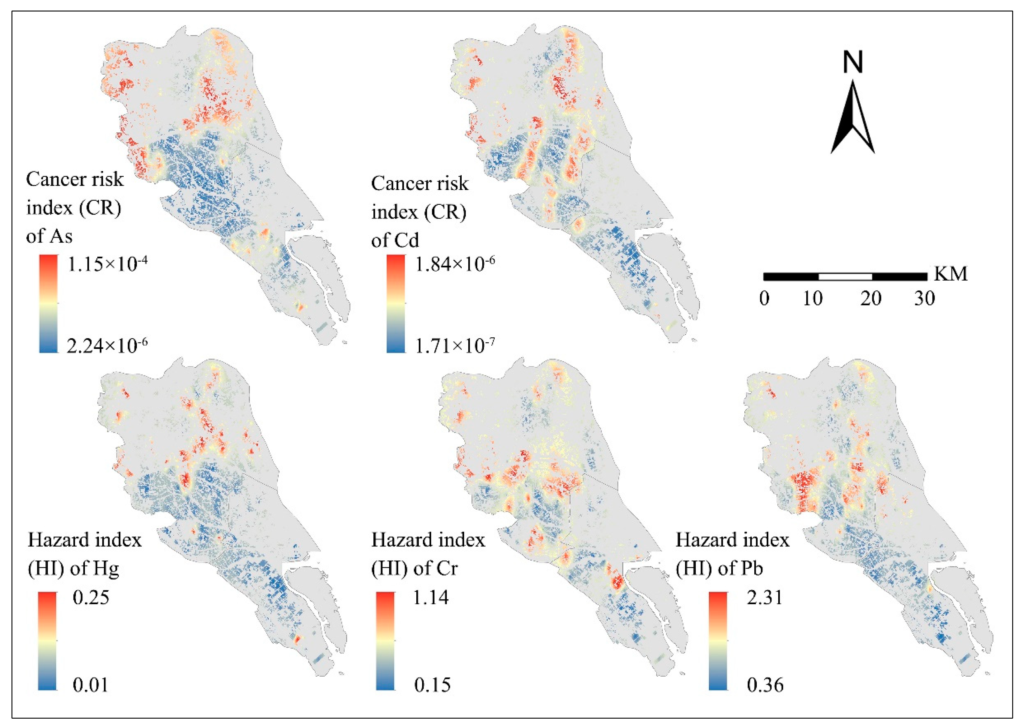
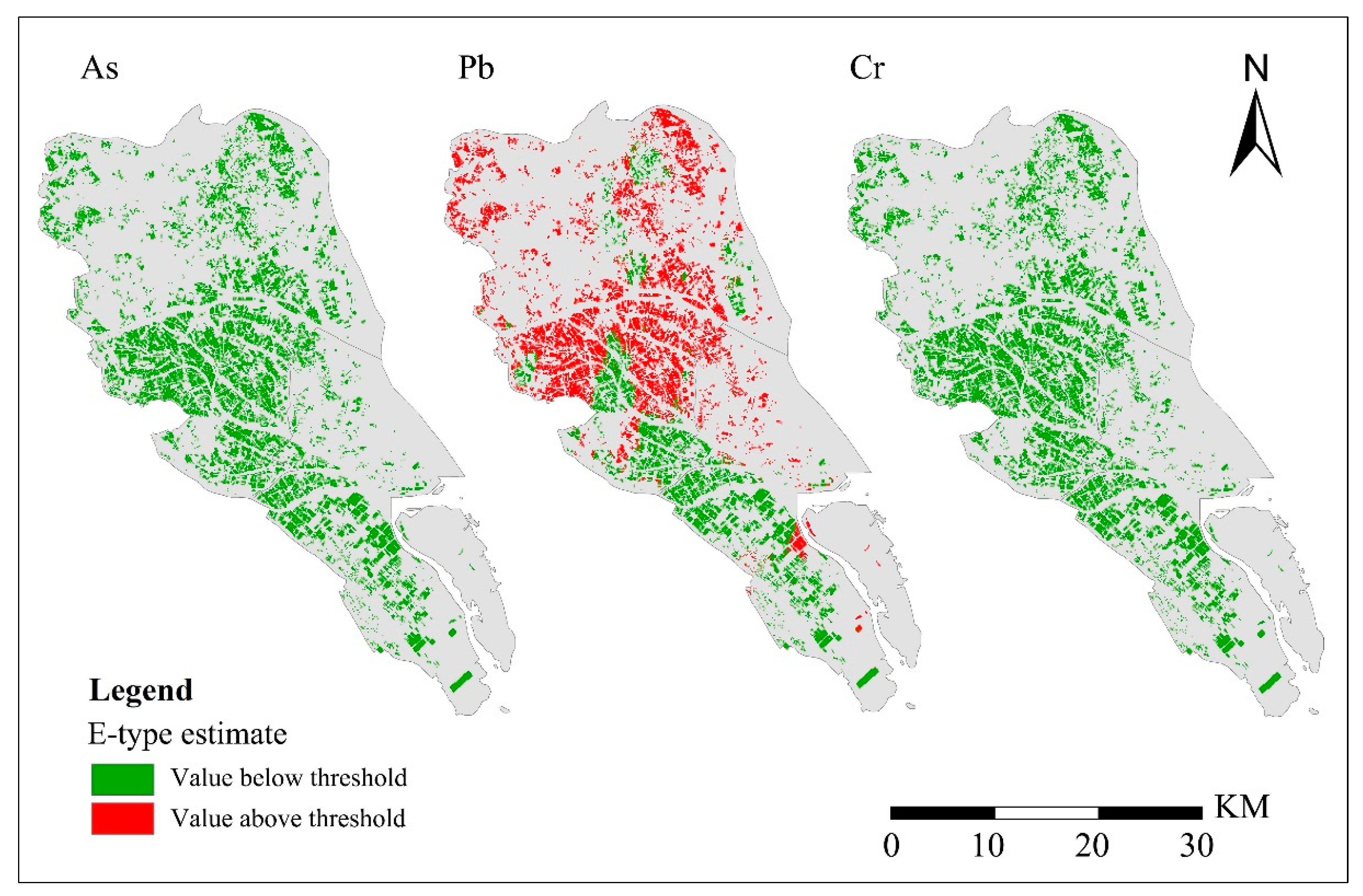
3.2.2. Human Health Risk Assessment Based on SIS

We used the thresholds (Table 2) to perform a sequential indicator simulation. This method needs the a priori information of the corresponding indicator Kriging. As the distribution of sample points was non-uniform, we used the average nearest neighbor method to determine the step size. According to the rule of thumb, the number of steps is equal to half the maximum distance between pairs of sample points divided by the step size. We took the quartile of each trace element concentrations as the threshold value, and obtained experimental semivariogram and variogram models of each threshold condition.

Table A4. Parameters of indicator semivariograms theoretical models for variables.

Element	Quantile	Threshold (mg/kg)	C0	C0 + C1	Fitted Model	Range(m)	R2
Cd	0.25	0.1440	0.1182	0.2704	Exponential	24,380	0.80
	0.5	0.1751	0.0710	0.2560	Gaussian	2760	0.90
	0.75	0.2208	0.0560	0.171	Gaussian	2060	0.91
Hg	0.25	0.0776	0.0001	0.1982	Exponential	1530	0.70
	0.5	0.1057	0.0082	0.2484	Exponential	1270	0.83
	0.75	0.1520	0.0569	0.1938	Spherical	21,920	0.96
AS	0.25	4.4085	0.0187	0.2014	Spherical	3210	0.65
	0.5	8.1937	0.1001	0.2962	Exponential	7460	0.95
	0.75	12.6000	0.0419	0.1948	Spherical	17,490	0.98
Pb	0.25	41.7199	0.1280	0.4010	Exponential	71,100	0.83
	0.5	48.9496	0.1194	0.2548	Exponential	2850	0.88
	0.75	57.9000	0.0607	0.1834	Exponential	1350	0.73
Cr	0.25	53.1686	0.1218	0.4286	Exponential	71,100	0.83
	0.5	69.3163	0.0863	0.2506	Exponential	1830	0.94
	0.75	87.6570	0.0264	0.1938	Exponential	510	0.60

lists the parameters of the experimental semivariograms and the fitted models for each trace element. According to the size of the study area and the operation time of grid division, we divided the study area into of 620 × 510 grid, where the size of each grid was 100 m × 100 m. We carried out 1000 realizations in each grid by SIS. Then, we obtained the risk index of CR or HI for each trace element by calculating the E-type estimates. The E-type estimates showed the spatial distribution of the risk index (Figure 2).

As shown by the risk index distribution map (Figure 2), the clusters with high values of each trace element were mostly concentrated in the north and central regions of the study area. These areas were mainly close to the Pearl River and the urban areas of the Panyu District (Figure 1). This showed that urban areas have an impact on trace elements of farmland around cities. The cancer risk index (CR) of As exceeded the threshold (10⁻⁴) in some areas. The cancer risk index (CR) of Cd did not exceed the threshold (10⁻⁴), which meant there was no risk of Cd in the study area. The maximum non-carcinogenic hazard index (HI) of Cr and Pb exceeded the threshold (1.0). In particular, the maximum non-carcinogenic HI of Pb was twice the standard threshold. The non-carcinogenic hazard index (HI) of Hg did not exceed the threshold (1.0), which meant there was no risk of Hg in the study area. According to the spatial distribution of risk index, the risk areas comprised only a small part of the study area.

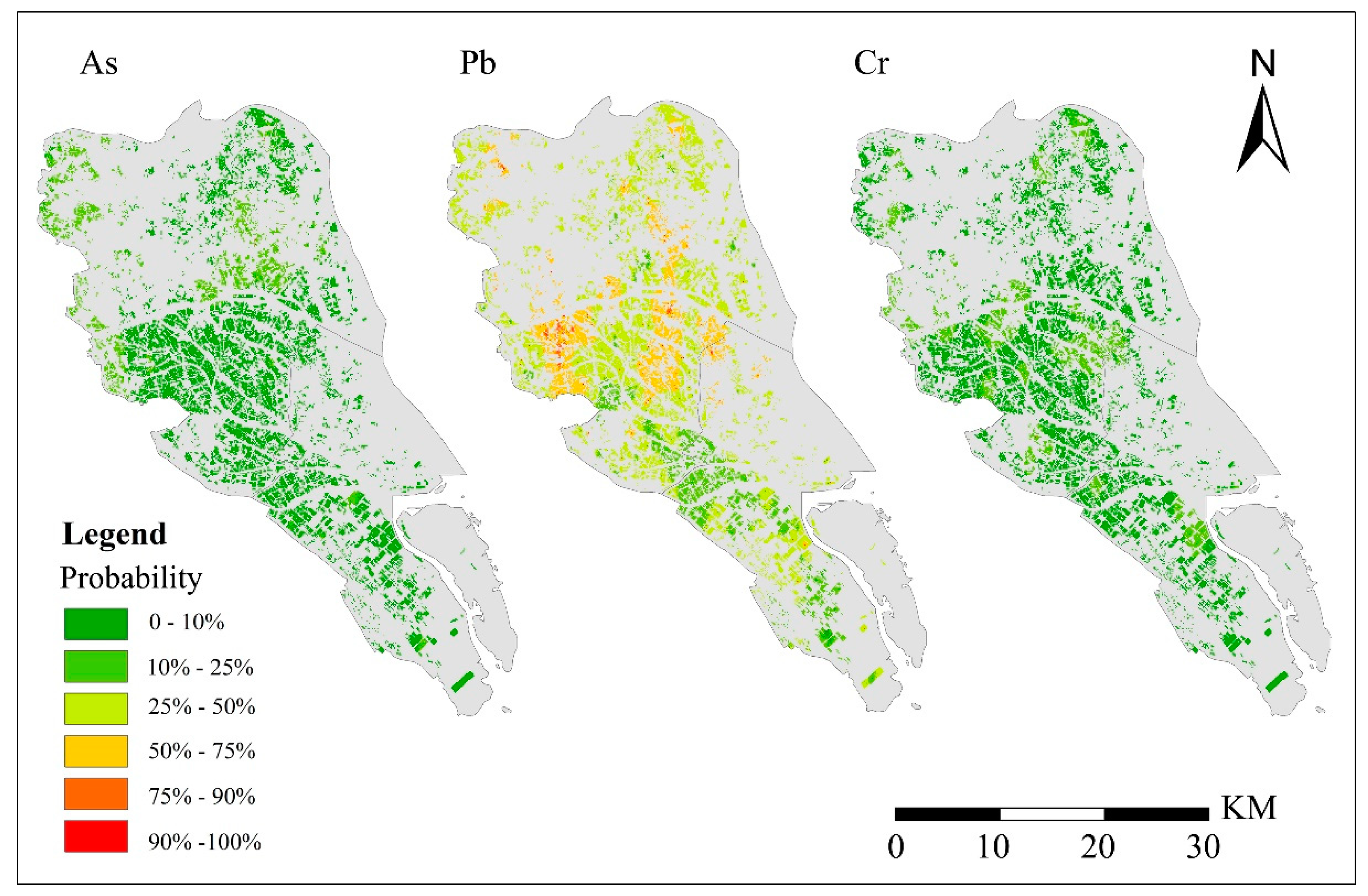
3.2.3. Uncertainty Assessment

From the above-mentioned CR or HI of trace elements, Cd and Hg were unlikely to pose a risk to human health in the study area. However, the maximum risk values of As, Pb, and Cr exceeded the threshold. We calculated the probability of each grid exceeding the risk for As, Pb, and Cr. The process was as follows: the risk threshold of each trace element was set as the criterion. Then, we counted the number (n₁) of each grid when the trace element concentration exceeded the risk threshold in n realizations; the risk probability of the grid was calculated with p = n₁/n. Figure 3 shows the spatial distribution of the risk probability.

Figure 3 shows that most of the risk probabilities of As and Cr ranged from 0% to 25%, which indicates a low-risk level. However, areas of high-risk probability (75% to 100%) also existed. The 100% risk probabilities for As and Cr only existed in a few grids. According to the size of the grid, a few parcels of farmland had certain health risks. Therefore, the overall risks of As and Cr were acceptable in the study area. We should give much more attention to the at-risk farmlands. Figure 3 also shows the risk probability of Pb. Most of the risk probabilities of Pb ranged from 25% to 50%, which indicates a moderate-risk level. The high-risk probability (75% to 100%) areas of Pb were concentrated in the central part of the study area. Furthermore, areas of 100% risk probability of Pb existed in some grids. The management should give priority to and carry out monitoring in these farmlands.

According to the grid statistics (Figure 4), most risk possibilities of As and Cr were less than 25%. Therefore, most areas were low-risk situations, which indicates that these trace elements were less likely to pose health risks in southern Guangzhou. The proportion of moderate-risk areas (25% < probability < 75%) for Pb was 80.06% in the study area. The proportion of high-risk areas (probability > 75%) for Pb was 1.2%, with an area of 2.8 km². Therefore, the study area had a moderate-risk of Pb. The risk probability can help to determine the key risk control areas of farmland. The management should set a certain monitoring threshold, and consider more sampling and analysis of toxic trace elements in these farmlands. It is necessary to take more protection measures in these farmlands.

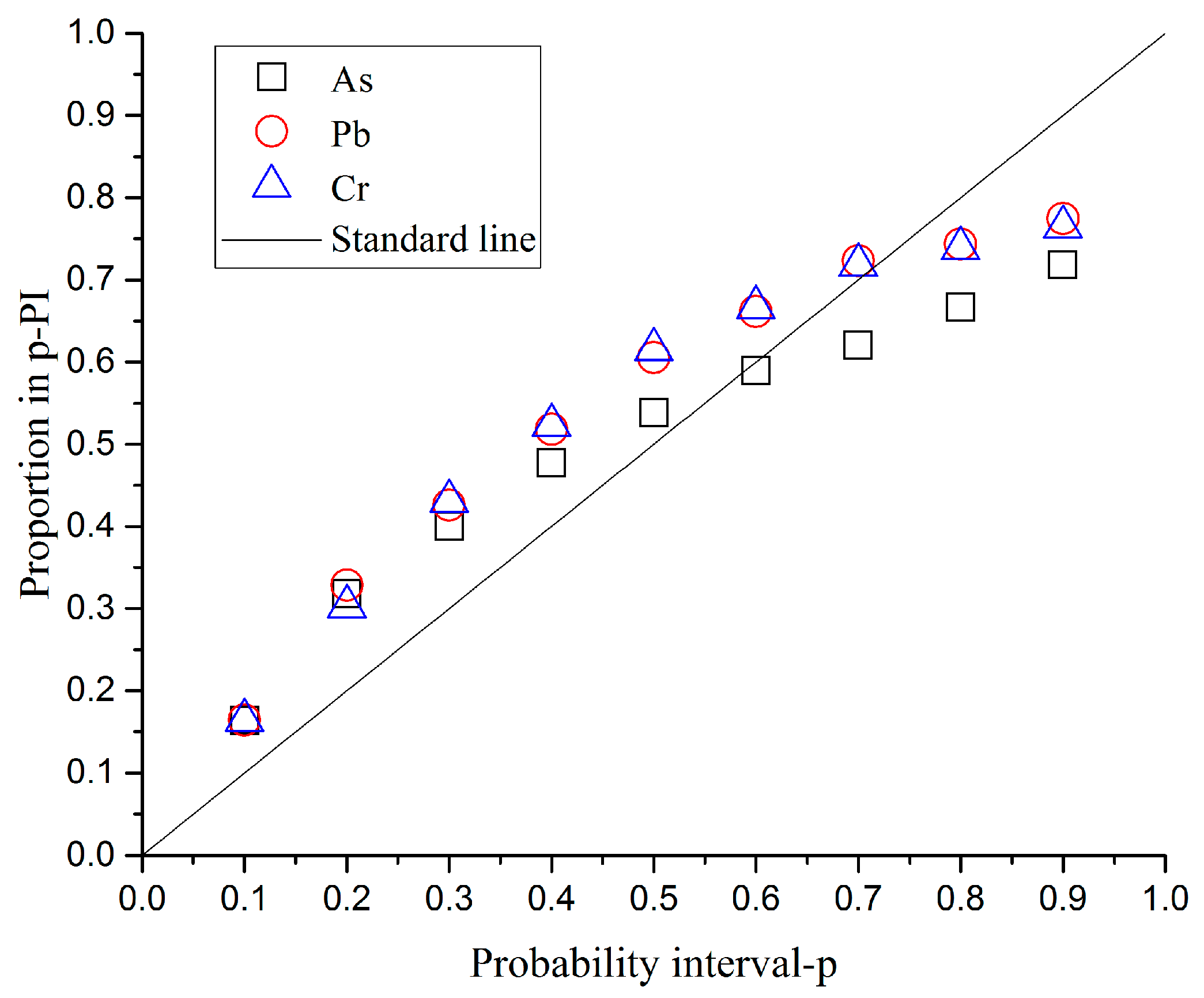
3.3. Accuracy Evaluation of the Uncertainty Model

We evaluated the accuracy of the risk uncertainty. Nine p-PI intervals (“10%”, “20%”, “30%”, “40%”, “50%”, “60%”, “70%”, “80%”, and “90%”) were calculated to obtain the probability that the sample point fell into the p interval. The closer the scatter is to the standard line (i.e., y = x), the more accurate the result. The results in Figure 5 show the accuracy of the evaluation results for the risk probability (CR or HI). The scattered lines are all close to the standard line. The RMSE level was also low: the RMSE of As, Pb, and Cr were 0.0218, 0.0208, and 0.0211, respectively. The RMSE indicated that the overall accuracy of the uncertainty evaluation was effective [39].

3.4. Discussion

3.4.1. Comparison of Human Health Risk Results

The coefficient variation (CV) of As was large, which means that the accumulation of As was mainly caused by human factors. The areas with high concentrations of As were close to the Pearl River basin in this study. The Panyu and Nansha District are delta areas where the sediments of the Pearl River accumulate, and the irrigation of the farmland in these areas depends on the Pearl River and its tributaries. The discharge of sewage and wastewater results in the increase of As concentrations in the Pearl River [43,44], which may cause the accumulation of As. At the same time, the productive process of Guangzhou’s non-ferrous metal production is the main source of As in the atmosphere. Dust deposition has a negative impact on outdoors environments, and the CR of As has been found to exceed the threshold in urban areas of Guangzhou [45], which is consistent with the results of this study. However, we also found that most of the risk of As did not exceed the unacceptable level in farmland of Guangzhou, and the risk management can be strengthened according to the risk probability.

From the results of the risk assessment for Cr, the risk probabilities of most farmlands were at a low-risk level (0%–25%). The health risk of Cr was found to be acceptable in Guangzhou City in other studies [18,45,46], in accordance with the results of this study. Very few farmlands exhibited a high-risk situation, and the spatial distribution did not show any tendency for aggregation. Therefore, we should analyze the high-risk fields, in order to determine if they are associated with point-source pollution.

Traffic activities have been shown to have a serious impact on the Pb pollution in the urban surface soil of Guangzhou [28,47]. The concentration of Pb in the soil has been positively correlated with the traffic load of the road [48]. The spatial distribution of Pb’s human health risk in farmland was scattered in this study. Most grids of risk probabilities (50%–100%) were near roads. In addition, most of these roads are expressways. Furthermore, Pb-containing substances enter the ground through industrial emission, coal combustion, and waste incineration [49,50]. Those problems also affect the farmland soil of this city. In this study, Pb is a toxic trace element which can pose health risks in some farmlands. Management should monitor the tendency of Pb accumulation to control the risk.

We found that there has no human health risk of Cd and Hg in the farmland soil of southern Guangzhou under the current conditions. In other studies on toxic trace elements in Guangzhou, the areas with high concentrations of Cd and Hg appeared in the core urban area of the city [51]. Those core urban areas are close to the north of the study area. At the same time, the human health risks of Cd and Hg in other studies were found to be acceptable for Guangzhou’s urban environment and atmospheric particles [18,52,53]. These conclusions were similar to our results.

3.4.2. Selection of Risk Mapping Based on the SIS Method

The SIS method can obtain the probability (above threshold) and conditional means (E-type estimate) for each variable grid [29]. Some studies have obtained the spatial distribution of regional trace element concentrations by using E-type estimates [3,14,31]. According to the risk threshold, the spatial distribution of regional trace element concentrations also can provide a reference for regional risk management [3,31].

We considered three kinds of numbers: the number of sample points whose sample concentration exceeded the risk threshold, the number of grids whose E-type estimated value exceeded the risk threshold, and the number of grids with 100% risk probability (

Table 3. Grid statistics for exceeding risk threshold of each trace element.

Elements	Sample Point	Grid Quantity (100%)	Grid Quantity (E-type)
As	3	3	3
Cr	1	1	1
Pb	73	65	14,614

). Combined with the spatial distribution of risk probability (Figure 3), locations of the sample concentration above the threshold were consistent with 100% risk probability locations. The numbers were equal or close for sample points and 100% risk probability grids. At the same time, the number and distribution (Figure 6) of over-risk grids (E-type estimate) of As and Cr were consistent with the over-risk sample point and the 100% risk probability grid. However, the number of over-risk grids (E-type estimate) of Pb were much greater than the 100% risk probability grid. This shows that these grids have a low risk probability but have a high E-type estimate value: which means that the high values in the grid have a small quantity, but a large contribution of the E-type estimate.

The risk threshold may have an impact on the accuracy of risk judgement made by the E-type estimate. Before the calculation of the E-type estimate, the sample data is divided into sub-intervals by quantiles. We then multiply the subinterval probability by the average of the subinterval to obtain the E-type estimate. The average value of the sub-interval is calculated by the head and tail values of these sub-intervals [54,55,56]. The number of sampling points whose sample concentration (Pb) exceeded the risk threshold was 42% of the total. We divided the Pb data into four sub-intervals (by quartile). We can see that the risk threshold was lower than the average of the third sub-interval (i.e., 2nd quartile to 3rd quartile). This is the reason why the E-type estimate is easily greater than the risk threshold. Therefore, when the number of samples with concentration above threshold has a large proportion of total sample amount, the E-type estimate overestimates the risk. Therefore, we tend to use the risk probability by using the SIS for risk judgement.

4. Conclusions

This study assessed the human health risks of toxic trace elements in the farmland of southern Guangzhou, a rapidly developing area of China. We also analyzed the risk uncertainty and visualized the regional risk probability. We drew the following conclusions.

The high-value areas of the human health risk index were concentrated in the north-central area (Panyun District) of the study area, which is close to the main urban area of Guangzhou, and has frequent human activities. We found that high urbanization poses a hazard to human health in farmland. We calculated the risk index of each trace element by using a risk assessment model of human health. The maximum risk indices of Cd and Hg were less than the standard threshold, while the maximum risk indices of As, Cr, and Pb exceeded the standard threshold. In particular, the maximum risk index of Pb was twice the standard threshold.

We visualized the risk uncertainty to obtain the risk probability distribution map. Most of the risk probabilities of As and Cr were between 0% and 25%, which indicates a low-risk level. The 100% human health risk probability areas of As and Cr were only a few parcels of farmland. Most of the risk probabilities of Pb were between 25% and 50%, which indicates a moderate-risk level. Some areas (2.8 km²) had a 100% probability health risk of Pb; we should give more attention and take more protection measures for farmland in these areas. The RMSE of the risk uncertainty model was low. The order of RMSE was As > Pb > Cr and the accuracy of the uncertainty model was acceptable.

We found that the mean estimate using traditional methods may underestimate the human health risks. Moreover, the E-type estimate by the SIS method overestimated the human health risk when the number of samples with concentration above the threshold had a large proportion of total sample amount. Therefore, we suggest using the risk probability by the SIS method to visualize regional human health risks. Using the risk probability makes interpreting the risk situation more intuitive. It is relatively reliable and realistic, and can provide guidance for the prevention of toxic trace elements influencing human health.

References

1. Foley, J.A.; DeFries, R.; Asner, G.P.; Barford, C.; Bonan, G.; Carpenter, S.R.; Chapin, F.S.; Coe, M.T.; Daily, G.C.; Gibbs, H.K.; et al. Global consequences of land use. Science 2005, 309, 570–574. [Google Scholar] [CrossRef] [Green Version]
2. Zhao, F.J.; Ma, Y.; Zhu, Y.G.; Tang, Z.; McGrath, S.P. Soil contamination in China: Current status and mitigation strategies. Environ. Sci. Technol. 2015, 49, 750–759. [Google Scholar] [CrossRef]
3. Zhao, H.; Xia, B.; Fan, C.; Zhao, P.; Shen, S. Human health risk from soil heavy metal contamination under different land uses near Dabaoshan Mine, Southern China. Sci. Total Environ. 2012, 417–418, 45–54. [Google Scholar] [CrossRef]
4. Järup, L. Hazards of heavy metal contamination. Br. Med. Bull. 2003, 68, 167–182. [Google Scholar] [CrossRef] [PubMed] [Green Version]
5. Lee, C.S.L.; Li, X.; Shi, W.; Cheung, S.C.N.; Thornton, I. Metal contamination in urban, suburban, and country park soils of Hong Kong: A study based on GIS and multivariate statistics. Sci. Total Environ. 2006, 356, 45–61. [Google Scholar] [CrossRef] [PubMed] [Green Version]
6. Cicchella, D.; DeVivo, B.; Lima, A.; Albanese, S.; McGill, R.A.R.; Parrish, R.R. Heavy metal pollution and Pb isotopes in urban soils of Napoli, Italy. Geochem. Explor. Environ. Anal. 2008, 8, 103–112. [Google Scholar] [CrossRef] [Green Version]
7. Sawut, R.; Kasim, N.; Maihemuti, B.; Hu, L.; Abliz, A.; Abdujappar, A.; Kurban, M. Pollution characteristics and health risk assessment of heavy metals in the vegetable bases of northwest China. Sci. Total Environ. 2018, 642, 864–878. [Google Scholar] [CrossRef] [PubMed]
8. Ho, Y.B.; Abdullah, N.H.; Hamsan, H.; Tan, E.S.S. Mercury contamination in facial skin lightening creams and its health risks to user. Regul. Toxicol. Pharmacol. 2017, 88, 72–76. [Google Scholar] [CrossRef]
9. Zukowska, J.; Biziuk, M. Methodological evaluation of method for dietary heavy metal intake. J. Food Sci. 2008, 73, R21–R29. [Google Scholar] [CrossRef]
10. Khan, A.G.; Kuek, C.; Chaudhry, T.M.; Khoo, C.S.; Hayes, W.J.; Wong, M.H. Role of plants, mycorrhizae and phytochelators in heavy metal contaminated land remediation. Chemosphere 2000, 41, 197–207. [Google Scholar] [CrossRef]
11. Yi, Y.; Yang, Z.; Zhang, S. Ecological risk assessment of heavy metals in sediment and human health risk assessment of heavy metals in fishes in the middle and lower reaches of the Yangtze River basin. Environ. Pollut. 2011, 159, 2575–2585. [Google Scholar] [CrossRef] [PubMed]
12. Gay, J.R.; Korre, A. A spatially-evaluated methodology for assessing risk to a population from contaminated land. Environ. Pollut. 2006, 142, 227–234. [Google Scholar] [CrossRef] [PubMed]
13. Khan, S.; Cao, Q.; Zheng, Y.M.; Huang, Y.Z.; Zhu, Y.G. Health risks of heavy metals in contaminated soils and food crops irrigated with wastewater in Beijing, China. Environ. Pollut. 2008, 152, 686–692. [Google Scholar] [CrossRef] [PubMed]
14. Zhao, Y.; Xu, X.; Sun, W.; Huang, B.; Darilek, J.L.; Shi, X. Uncertainty assessment of mapping mercury contaminated soils of a rapidly industrializing city in the Yangtze River Delta of China using sequential indicator co-simulation. Environ. Monit. Assess. 2008, 138, 343–355. [Google Scholar] [CrossRef] [PubMed]
15. Zhuang, P.; McBride, M.B.; Xia, H.; Li, N.; Li, Z. Health risk from heavy metals via consumption of food crops in the vicinity of Dabaoshan mine, South China. Sci. Total Environ. 2009, 407, 1551–1561. [Google Scholar] [CrossRef] [PubMed]
16. Man, Y.B.; Sun, X.L.; Zhao, Y.G.; Lopez, B.N.; Shanshan, C.; Wu, S.C.; Kwaichung, C.; Wong, M.H. Health risk assessment of abandoned agricultural soils based on heavy metal contents in Hong Kong, the world’s most populated city. Environ. Int. 2010, 36, 570–576. [Google Scholar] [CrossRef]
17. Li, P.; Lin, C.; Cheng, H.; Duan, X.; Lei, K. Contamination and health risks of soil heavy metals around a lead/zinc smelter in southwestern China. Ecotoxicol. Environ. Saf. 2015, 113, 391–399. [Google Scholar] [CrossRef]
18. Gu, Y.G.; Gao, Y.P.; Lin, Q. Contamination, bioaccessibility and human health risk of heavy metals in exposed-lawn soils from 28 urban parks in southern China’s largest city, Guangzhou. Appl. Geochem. 2016, 67, 52–58. [Google Scholar] [CrossRef]
19. MEPPRC. Technical Guidelines for Risk Assessment of Contaminated Sites (HJ25.3-2014, Published in Chinese); China Environmental Science Press: Beijing, China, 2014. [Google Scholar]
20. Chen, H.; Teng, Y.; Lu, S.; Wang, Y.; Wu, J.; Wang, J. Source apportionment and health risk assessment of trace metals in surface soils of Beijing metropolitan, China. Chemosphere 2015, 144, 1002. [Google Scholar] [CrossRef]
21. Schuhmacher, M.; Meneses, M.; Xifró, A.; Domingo, J.L. The use of Monte-Carlo simulation techniques for risk assessment: study of a municipal waste incinerator. Chemosphere 2001, 43, 787. [Google Scholar] [CrossRef]
22. Sonnemann, G.W.; Pla, Y.; Schuhmacher, M.; Castells, F. Framework for the uncertainty assessment in the Impact Pathway Analysis with an application on a local scale in Spain. Environ. Int. 2002, 28, 9–18. [Google Scholar] [CrossRef]
23. Pyrcz, M.J.; Deutsch, C. V Geostatistical Reservoir Modeling; Oxford University Press: New York, NY, USA, 2014; ISBN 0199731446. [Google Scholar]
24. Albuquerque, M.T.D.; Gerassisc, S.; Sierrad, C.; Taboadac, J.; Martínc, J.E.; Antuneseb, I.M.H.R. Developing a new Bayesian Risk Index for risk evaluation of soil contamination. Sci. Total Environ. 2017, 603–604, 167–177. [Google Scholar] [CrossRef] [PubMed]
25. Goovaerts, P. Geostatistics for Natural Resources Evaluation; Oxford University Press: New York, NY, USA, 1997. [Google Scholar]
26. Duzgorenaydin, N.S.; Wong, C.S.; Aydin, A.; Song, Z.; You, M.; Li, X.D. Heavy metal contamination and distribution in the urban environment of Guangzhou, SE China. Environ. Geochem. Health 2006, 28, 375–391. [Google Scholar] [CrossRef] [PubMed]
27. Li, J.H.; Ying, L.; Wei, Y.; Gan, H.H.; Chao, Z.; Deng, X.L.; Jin, L. Distribution of heavy metals in agricultural soils near a petrochemical complex in Guangzhou, China. Environ. Monit. Assess. 2009, 153, 365–375. [Google Scholar] [CrossRef] [PubMed]
28. Cai, Q.Y.; Mo, C.H.; Li, H.Q.; Lü, H.; Zeng, Q.Y.; Li, Y.W.; Wu, X.L. Heavy metal contamination of urban soils and dusts in Guangzhou, South China. Environ. Monit. Assess. 2013, 185, 1095–1106. [Google Scholar] [CrossRef]
29. Goovaerts, P. Geostatistical modelling of uncertainty in soil science. Geoderma 2001, 103, 3–26. [Google Scholar] [CrossRef]
30. Juang, K.W.; Chen, Y.S.; Lee, D.Y. Using sequential indicator simulation to assess the uncertainty of delineating heavy-metal contaminated soils. Environ. Pollut. 2004, 127, 229–238. [Google Scholar] [CrossRef]
31. Huang, J.; Liu, W.; Zeng, G.; Li, F.; Huang, X.; Gu, Y.; Shi, L.; Shi, Y.; Wan, J. An exploration of spatial human health risk assessment of soil toxic metals under different land uses using sequential indicator simulation. Ecotoxicol. Environ. Saf. 2016, 129, 199–209. [Google Scholar] [CrossRef]
32. Deutsch, C.V.; Journel, A.G. GSLIB: Geostatistical Software Library and User’s Guide, 2nd ed.; Oxford University Press: New York, NY, USA, 1998. [Google Scholar]
33. Cattle, J.A.; McBratney, A.; Minasny, B. Kriging method evaluation for assessing the spatial distribution of urban soil lead contamination. J. Environ. Qual. 2002, 31, 1576–1588. [Google Scholar] [CrossRef]
34. Chen, H.; Teng, Y.; Lu, S.; Wang, Y.; Wang, J. Contamination features and health risk of soil heavy metals in China. Sci. Total Environ. 2015, 512, 143–153. [Google Scholar] [CrossRef]
35. US EPA. Proposed Guidelines for Carcinogen Risk Assessment. Fed. Regist. 1996, 61, 17960–18011. [Google Scholar]
36. Pawełczyk, A.; Božek, F.; Grabas, K. Impact of military metallurgical plant wastes on the population’s health risk. Chemosphere 2016, 152, 513–519. [Google Scholar] [CrossRef] [PubMed]
37. Katz, S.A.; Salem, H. The Biological and Environmental Chemistry of Chromium; Wiley Sons: Hoboken, NJ, USA, 1994. [Google Scholar]
38. US EPA Regional Screening Levels (RSLs). Available online: https://www.epa.gov/risk/regional-screening-levels-rsls (accessed on 1 December 2018).
39. Yang, Y.; Christakos, G. Uncertainty assessment of heavy metal soil contamination mapping using spatiotemporal sequential indicator simulation with multi-temporal sampling points. Environ. Monit. Assess. 2015, 187, 571. [Google Scholar] [CrossRef] [PubMed]
40. AQTSGP. Risk Screening Values for Soil Heavy Metal The Pearl River Delta Area (DB 44/ T1415--2014, Published in Chinese); Guangdong Quality and Technical Supervision Bureau: Guangzhou, China, 2014. [Google Scholar]
41. Li, F.; Huang, J.; Zeng, G.; Liu, W.; Huang, X.; Huang, B.; Gu, Y.; Shi, L.; He, X.; He, Y. Toxic metals in topsoil under different land uses from Xiandao District, middle China: distribution, relationship with soil characteristics, and health risk assessment. Environ. Sci. Pollut. Res. Int. 2015, 22, 12261–12275. [Google Scholar] [CrossRef]
42. Yao, R.; Yang, J.; Han, J. Stochastic simulation and uncertainty assessment of spatial variation in soil salinity in coastal reclamation regions. Zhongguo Shengtai Nongye Xuebao/Chinese J. Eco-Agriculture 2011, 19, 485–490. [Google Scholar] [CrossRef]
43. Wang, S.; Cao, X.; Lin, C.; Chen, X. Arsenic content and fractionation in the surface sediments of the Guangzhou section of the Pearl River in Southern China. J. Hazard. Mater. 2010, 183, 264–270. [Google Scholar] [CrossRef]
44. Han, L.; Gao, B.; Hao, H.; Lu, J.; Xu, D. Arsenic pollution of sediments in China: An assessment by geochemical baseline. Sci. Total Environ. 2019, 651, 1983–1991. [Google Scholar] [CrossRef]
45. Huang, M.; Wang, W.; Chan, C.Y.; Cheung, K.C.; Man, Y.B.; Wang, X.; Wong, M.H. Contamination and risk assessment (based on bioaccessibility via ingestion and inhalation) of metal (loid) s in outdoor and indoor particles from urban centers of Guangzhou, China. Sci. Total Environ. 2014, 479, 117–124. [Google Scholar] [CrossRef]
46. Gu, Y.G.; Gao, Y.P. Bioaccessibilities and health implications of heavy metals in exposed-lawn soils from 28 urban parks in the megacity Guangzhou inferred from an in vitro physiologically-based extraction test. Ecotoxicol. Environ. Saf. 2018, 148, 747–753. [Google Scholar] [CrossRef]
47. Duzgoren-Aydin, N.S. Sources and characteristics of lead pollution in the urban environment of Guangzhou. Sci. Total Environ. 2007, 385, 182–195. [Google Scholar] [CrossRef]
48. Pariente, S.; Helena, Z.; Eyal, S.; Anatoly, F.G.; Michal, Z. Road side effect on lead content in sandy soil. Catena 2019, 174, 301–307. [Google Scholar] [CrossRef]
49. Lu, J.; Ma, L.; Cheng, C.; Pei, C.; Chan, C.K.; Bi, X.; Qin, Y.; Tan, H.; Zhou, J.; Chen, M. Real time analysis of lead-containing atmospheric particles in Guangzhou during wintertime using single particle aerosol mass spectrometry. Ecotoxicol. Environ. Saf. 2019, 168, 53–63. [Google Scholar] [CrossRef] [PubMed]
50. Bi, C.; Zhou, Y.; Chen, Z.; Jia, J.; Bao, X. Heavy metals and lead isotopes in soils, road dust and leafy vegetables and health risks via vegetable consumption in the industrial areas of Shanghai, China. Sci. Total Environ. 2018, 619, 1349–1357. [Google Scholar] [CrossRef] [PubMed]
51. Li, C.; Sun, G.; Wu, Z.; Zhong, H.; Wang, R.; Liu, X.; Guo, Z.; Cheng, J. Soil physiochemical properties and landscape patterns control trace metal contamination at the urban-rural interface in southern China. Environ. Pollut. 2019, 250, 537–545. [Google Scholar] [CrossRef] [PubMed]
52. Huang, M.; Chen, X.; Shao, D.; Zhao, Y.; Wang, W.; Wong, M.H. Risk assessment of arsenic and other metals via atmospheric particles, and effects of atmospheric exposure and other demographic factors on their accumulations in human scalp hair in urban area of Guangzhou, China. Ecotoxicol. Environ. Saf. 2014, 102, 84–92. [Google Scholar] [CrossRef] [PubMed]
53. Huang, M.; Wang, W.; Leung, H.; Chan, C.Y.; Liu, W.K.; Wong, M.H.; Cheung, K.C. Mercury levels in road dust and household TSP/PM2. 5 related to concentrations in hair in Guangzhou, China. Ecotoxicol. Environ. Saf. 2012, 81, 27–35. [Google Scholar] [CrossRef]
54. Xiao, S.; Zhao, Y.; Wang, B. Problem analysis of geological properties evaluation using indicator Kriging. Petrochem. Ind. Appl. 2013. [Google Scholar]
55. Antunes, I.M.H.R.; Albuquerque, M.T.D. Using indicator kriging for the evaluation of arsenic potential contamination in an abandoned mining area (Portugal). Sci. Total Environ. 2013, 442, 545–552. [Google Scholar] [CrossRef]
56. Journel, A.G. Nonparametric estimation of spatial distributions. J. Int. Assoc. Math. Geol. 1983, 15, 445–468. [Google Scholar] [CrossRef]
Figure 1. Sample point spatial distribution map.
Sustainability 12 03852 g001
Figure 2. Spatial distribution of the cancer risk index (CR) or non-carcinogenic hazard index (HI) for each trace element.
Sustainability 12 03852 g002
Figure 3. Spatial distribution for the risk probability of each trace element.
Sustainability 12 03852 g003
Figure 4. Grid statistics of risk probabilities of As, Pb, and Cr.
Sustainability 12 03852 g004
Figure 5. Scatter plot of p-PI and risk probability.
Sustainability 12 03852 g005
Figure 6. Spatial distribution of E-type estimate for risk threshold of each trace element.
Sustainability 12 03852 g006