AI-Based Campus Energy Use Prediction for Assessing the Effects of Climate Change

Abstract

In developed countries, buildings are involved in almost 50% of total energy use and 30% of global annual greenhouse gas emissions. The operational energy needs of buildings are highly dependent on various building physical, operational, and functional characteristics, as well as meteorological and temporal properties. Besides physics-based energy modeling of buildings, Artificial Intelligence (AI) has the capability to provide faster and higher accuracy estimates, given buildings’ historic energy consumption data. Looking beyond individual building levels, forecasting building energy performance can help city and community managers have a better understanding of their future energy needs, and to plan for satisfying them more efficiently. Focusing at an urban scale, this research develops a campus energy use prediction tool for predicting the effects of long-term climate change on the energy performance of buildings using AI techniques. The tool comprises four steps: Data Collection, AI Development, Model Validation, and Model Implementation, and can predict the energy use of campus buildings with 90% accuracy. We have relied on energy use data of buildings situated in the University of Florida, Gainesville, Florida (FL). To study the impact of climate change, we have used climate properties of three future weather files of Gainesville, FL, developed by the North American Regional Climate Change Assessment Program (NARCCAP), represented based on their impact: median (year 2063), hottest (2057), and coldest (2041).

1. Introduction

1.1. Climate Change and Building Energy

The Third United States National Climate Assessment [1] describes climate change consisting of long-term variations in temperature, wind, precipitation, and all other aspects of the Earth climate. In the 21th century, the Earth temperature increase is likely to be the largest among any century in the past ten centuries. There are robust indications that the average temperature of Earth will increase for 2 °C in the 21st century [2]. Although this amount of change may sound insignificant, it can cause considerable changes in the Earth’s climate and disturb its natural weather systems. As a result, extensive drought and reduced crops, rapid and considerable rise in sea levels, and stronger hurricanes and cyclones are highly probable and soon would threaten human survival. According to the Intergovernmental Panel on Climate Change (IPCC) geological records, passing 450 ppm average CO₂ concentration means an ice-free planet with water levels 220 feet higher than today. Continuing business as usual will likely increase the CO₂ concentration levels to pass 450 ppm by 2050 [2].

Globally, buildings are involved in almost 50% of total energy usage and 30% of annual greenhouse gas emissions [3]. According to the International Energy Agency [4], in the United States nationwide, buildings account for 39% of total energy consumption, 30% of Global Warming Potential (GWP), 30% of raw materials consumption, 30% of waste, 12% of water usage, and 68% of electricity usage. Also, the primary source for satisfying the electricity demands of buildings are power plants which utilize water for functioning. Based on research conducted by the US Geological Survey in 2000 [5], 52% of total surface water and 39% of all freshwater withdrawals were consumed for thermoelectric power generation in power plants in that year.

In the European Union (EU), residential buildings consume 22% of total energy. Policy makers have recognized this sector’s potential to contribute towards lowering energy consumption and CO₂ emissions. Therefore, several policies and directives were issued in order to enhance building energy performance [6]. The main purpose of such policies is to promote the improvements of building energy performance through requirements such as calculation of integrated energy performance of buildings, application of minimum criteria for new and renovated buildings, energy performance certifications, and HVAC systems inspection [7]. In United Kingdom (UK), CO₂ emissions are set to be reduced by at least 26% by 2020 and 80% by 2050, compared to 1990 levels [8]. Another example is the Committee on Climate Change (CCC) that defined a series of carbon budgets in order to create the background for meeting 2050-desired CO₂ levels in each contributing sector [9].

During recent decades, a vast range of national-level building energy demand models were developed in a disaggregated way, varying considerably regarding data input requirements and sociotechnical assumptions about building operation [10]. Therefore, their expected results vary considerably based on these assumptions. However, a better understanding of the limitations and capabilities of these models would benefit both building scientists and policy makers. Such knowledge would help policy makers to determine which building parameters are important for national carbon reduction and to come up with more effective adaptation strategies [7]. Furthermore, construction professionals could also benefit from this knowledge in developing techniques and business strategies for sustainable refurbishment.

1.2. Urban Building Energy Consumption

According to the United Nations World Population Prospects [11], by 2050, two-thirds of the world’s population will be urban, increasing the negative effects of climate change and the importance of seeking practical solutions. Global energy and environmental challenges have led city governments to gradually modify their policies, decisions, and strategies towards greener and energy efficient approaches. In the U.S., state governments have set ambitious goals in reducing their Greenhouse Gas (GHG) emissions, such as 80% by 2050 in New York City [12] and Boston [13]. Besides understanding current consumption patterns, forecasting urban building energy performance is crucial to meeting such goals.

Considering the potentials beyond individual building scale, urban planners, civil engineers, and construction managers can considerably contribute to form energy efficient cities [14]. However, the problem includes complex details, making the solution difficult [15]. Currently, both planning and research communities agree that there is an urgent need for a new understanding of the role of urban planning in dealing with these rising issues. Moving above the common tasks of defining strategic plans and designing a city’s spatial aspects, urban planners must carefully address energy and resource management issues simultaneously [15]. Increasing interests in accurate building energy performance simulation tools, as well as the traditional focus on developing certification procedures, shows the interests of experts and researchers in assessing the energy performance of individual buildings rather than large building stocks. However, in order to achieve the desired global environmental goals, it is extremely important to focus on evaluating the energy performance of buildings at a regional, urban, or national scale [14].

1.3. Building Energy Performance Forecasting (BEPF)

Improvements in computer technology have made computers reliable and common tools in optimizing building design and assessment of their performance. Also, the speed and accuracy of computer calculations make them important tools, contributing to the engineering of a building’s life cycle [16]. As a result, computer simulations are extensively implemented in the design and operation of buildings [17]. Among them, energy simulation models are essentially used in BEPF. However, optimization models are not frequently used in designing building energy performance, due to the complexity of building systems and their dynamic thermal behavior [16]. Yet, as today’s computers are growing more capable, systematic prediction and optimization approaches are becoming more feasible to achieve in building energy performance assessment and design [14].

Accurate energy forecasting methods have various advantages in planning and optimization of building energy demands at individual or urban scale. For new buildings, which do not have any energy consumption history, computer simulation methods are implemented for energy analysis and forecasting possible future scenarios [18]. However, for existing buildings with available historic time series energy data, statistical and machine learning approaches can be faster and much more accurate [19].

Common computer software and regulations are typically very effective in assessing the energy performance of new buildings. However, once the building is operating, various factors with complex interactions influence its energy behavior. Due to such interactions, accurate simulation of buildings using energy simulation software is extremely difficult [17]. Therefore, the use of data-driven techniques can fundamentally help in assessing the energy performance of existing buildings [20,21,22,23,24]. These techniques rely on a building’s historic data in order to model its future energy use patterns. The main advantages of the data-driven approach are fast computation of real time data, being suitable for nonlinear modeling, and higher accuracy levels comparing to deterministic models [25]. However, data-driven approaches are highly dependent on historic data, difficult to generalize, and nontransparent [26,27].

Focusing on data-driven techniques, this research develops a Campus Energy Use Prediction (CEUP) tool for predicting the effects of long-term climate change on building energy performance using artificial intelligence. According to our results:

• CEUP model can predict the energy use of campus buildings with 90% accuracy;
• University of Florida (UF) campus energy use in the upcoming 40 years, based on the North American Regional Climate Change Assessment Program (NARCCAP) future weather scenarios, can be up to 20% higher;
• Among climatic and temporal variables, average outdoor temperature is a good measure to predict hourly energy consumption of campus buildings;
• Space functionality characteristics of various buildings in accurate gross square feet percentages are used as one of the inputs to our prediction model;
• Incorporating building functionalities in space-level can increase the accuracy of physics-based building clustering and hence result in better prediction accuracy.

2. Background

Machine Learning Applications in BEPF

In a systematic approach, we reviewed recent studies published since 2015, regarding the applications of machine learning (ML) in individual and urban level BEPF, according to five criteria of learning method, building type, energy type, input data, and time scale [28]. Various levels of these criteria were used for applying ML methods in BEPF, and there was no solid proof or measure that a specific method or criterion performs better than the others. Reviewing more than 70 journal papers in this field, we found that the majority of BEPF studies focus on combining or comparing various ML methods, as well as categorizing building functionality, characteristics, and consumption patterns. Out of all the articles, 61% focused on individual building level, while 39% were conducted on an urban level. The scarcity of research in urban versus individual level ML-based BEPF is considerable.

Most literature focused on predicting electricity (44%), heating and cooling energy (39%), and total building energy (29%) in both individual and urban levels, while only 2% considered natural gas in their studies. In urban level studies, predicting building total energy use was more popular among researchers, while in individual level, more ML-based methods were used for predicting electricity and heating and cooling energy consumption. Commercial, residential, and educational buildings were studied in 54%, 39%, and 26% of recent BEPF literature, respectively, addressing the relative preference of researchers in studying these three types of buildings, mainly due to the availability and reliability of building consumption and characteristics data. Cluster Analysis (CA) methods were used more frequently in urban level BEPF, due to their capacities in categorizing various buildings in a diverse environment.

Among recent studies on educational buildings, none studied several educational buildings in a campus order. In our initial attempt to address this issue, we evaluated the energy performance of two buildings representing a section of UF campus buildings. A set of energy efficiency measures were identified and implemented, assessing their effects on building energy performance [29]. Comparing various time scales, we noticed that hourly prediction resolution was more frequently used in individual level BEPF, while annual prediction resolution was more frequently used in urban level BEPF. As information systems management software, hardware, and practices are enhanced, we observe more studies being conducted on hourly and subhourly ML-based BEPF in urban and community levels.

Meteorological, occupancy, and temporal data were used much more frequently in BEPF research, compared to the other input data types, while building functionality and spatial properties were only used in urban scale studies. Considering the meteorological input data type, which was used in 65% of all BEPF studies, it is really important to understand the capacities of such input in climate change adaptation practices, as they could be used as controlling variables in order to adapt to various climate scenarios. Comparing input data types in individual level BEPF, we noticed that meteorological data were used much more frequently as learning inputs, compared to all other input data types. Such focus was not extensive in urban level studies. Accordingly, future urban level BEPF studies can focus more on simulation based on meteorological data, to be able to further enhance climate change adaptation practices. In the literature reviewed, there was no study that assessed the effects of climate change on community building energy performance using future weather scenarios, as well as addressing adaptation strategies or design resiliency. In order to fill this research gap, we propose the following method.

3. Methodology

This research develops a Campus Energy Use Prediction (CEUP) tool for predicting the effects of long-term climate change on the energy performance of buildings using AI techniques. Figure 1 shows the general structure of CEUP that we developed in this study. The CEUP model uses a four-layer structure consisting of (1) Data Collection, (2) AI Development, (3) Model Validation, and (4) Model Implementation, and can predict the energy use of campus buildings with 90% accuracy. We relied on energy use data of buildings at the University of Florida, Gainesville, Florida (FL).

Layer 1 refers to collecting a building’s specification data, as well as its total monthly and hourly utility consumption, consisting of electricity, chilled water, steam, and natural gas. In addition, local monthly and hourly average outdoor temperature, relative humidity, and solar radiation were collected for the UF Campus. In layer 2, the AI-based energy use prediction model was developed using k-means clustering, Principal Component Analysis (PCA), Auto-Regressive Integrated Moving Average (ARIMA), polynomial regression analysis, and Long Short-Term Memory (LSTM) techniques. In layer 3, the CEUP model was validated using actual energy consumption for a cluster of representative buildings on campus. Finally, in the fourth layer, campus energy use was predicted using three future climate scenarios. To study the impact of climate change, we used climate properties of three future weather files of Gainesville, FL, developed by the North American Regional Climate Change Assessment Program (NARCCAP) represented and based on their average outdoor air temperature, relative humidity, and solar radiation: median (year 2063), hottest (year 2057), and coldest (year 2041). In order to conduct the scenario analysis, we referred to the Technology Roadmap—Energy Efficient Building Envelopes (International Energy Agency (IEA), 2013) [30], which is used to assess and present the development of technology products in the building sector. According to the roadmap, we assessed campus energy use for five envelope scenarios for each of the future climate scenarios. Each layer is explained in more detail in the following sections.

4. Model Development and Results

4.1. Layer 1: Data Collection

University of Florida (UF) has an 800 hectare campus and more than 900 buildings. According to the campus utility data obtained from UF’s Physical Plant Division (PPD), there are a total of 217 buildings with a sensor configuration that captures an individual building’s utility consumption every 15 minutes. UF also provided access to the documentation of the building’s energy performance for various energy performance rating systems, such as the US Green Building Council’s (USGBC) Leadership in Energy and Environmental Design (LEED) rating system. Reviewing energy rating documentation varying from preliminary design plans to as-built plans and LEED V4 (release date: Nov. 2013) forms, we could derive some of the thermophysical properties that influence building energy performance. Twelve buildings had the required information available. The set includes various primary building functions, such as educational, residential, research laboratory, and sport facilities. Four types of data were collected for this research: (A) space functionality characteristics; (B) building thermophysical properties, including lighting and equipment energy intensities; (C) building energy use; and (D) historic and future weather data.

(A) Space functionality characteristics were determined using the percentages of different functional spaces in every building, which were calculated for each building used in this study. Offices, classrooms, teaching labs, research areas, auditoriums, gymnasiums, and residential areas are some of the functional spaces used for this classification. For instance, Rinker Hall (Bldg. ID 0272), which houses UF’s School of Construction Management, consists of 14% classrooms and 25% office areas, while Hough Graduate School of Business (Bldg. ID 0064) has 21% office areas and 22% classrooms. The space classification percentages were based on the Gross Square Feet (GSF) area of the buildings [29].

Table 1. Building space functionality percentages.

Bldg. ID	Total GSF	Classroom (%)	Teaching Labs (%)	Study Room (%)	Research Lab (%)	Office (%)	Auditorium (%)	Instructor Media (%)	Academic Supply (%)	Campus Supply (%)	Residential (%)	Sport (%)	Unconditioned (%)
0028	88,732	5.5	0.0	0.0	50.5	11.7	0.0	0.0	0.0	0.0	0.0	0.0	32.3
0064	72,724	21.5	0.6	3.2	0.0	20.6	0.0	0.3	0.0	0.0	0.0	0.0	53.8
0081	23,635	1.4	0.0	1.4	0.0	51.7	0.0	0.7	0.0	0.0	0.0	0.0	44.8
0086	85,155	0.0	0.0	0.0	0.0	5.2	0.0	0.0	0.0	0.0	56.1	0.0	38.7
0110	17,032	53.5	0.0	7.5	0.0	10.1	0.0	0.0	0.0	0.0	0.0	0.0	28.9
0214	85,486	20.0	13.5	7.0	0.5	12.1	1.5	0.0	0.0	0.0	0.0	0.0	45.4
0272	56,352	14.4	18.6	0.0	0.0	25.2	0.0	0.0	0.0	0.8	0.0	0.0	41.0
0289	18,410	0.0	0.0	0.0	0.0	0.0	0.0	0.0	0.0	0.0	66.5	0.0	33.5
0764	19,375	26.1	19.0	0.0	0.0	12.5	0.0	0.0	0.0	0.0	0.0	0.0	42.4
0860	84,804	0.0	0.0	0.0	0.0	0.0	0.0	0.0	0.0	0.0	0.0	99.0	1.0
1375	119,763	0.0	1.4	0.4	1.0	32.1	5.3	0.0	0.0	0.0	0.0	0.0	59.8
1377	93,018	0.0	0.0	0.0	31.4	24.8	0.0	0.0	0.0	0.7	0.0	0.0	43.1

represents the list of space functionality percentages used in this study. Note that space functionalities like campus supply, residential, or sport that were mostly zero for the selected buildings were removed from the study in later sections.

(B) The building thermophysical properties that we could derive from the energy performance documents, and can be seen in

Table 2. Building thermophysical properties.

Bldg. ID	Total Gross Square Meter (GSM) (m2)	Number of Floors	Window to Wall (W/W) Ratio	Exterior Wall U-value (W/m2 °C)	Windows U-value (W/m2 °C)	Windows Solar Heat Gain Coefficient (SHGC)	Roof U-value (W/m2 °C)	Lighting Power Density (LPD) (W/m2)	Equipment Power Density (EPD) (W/m2)
0028	8243	2	0.138	0.3878	3.0810	0.30	0.2714	6.1354	18.08334
0064	6756	4	0.203	0.2220	5.1104	0.50	0.1447	9.9162	10.7639
0081	2196	3	0.19	0.2986	1.5331	0.38	0.2839	13.4548	16.1459
0086	7911	5	0.254	0.2285	2.4416	0.24	0.1493	5.9202	9.6875
0110	1582	2	0.072	0.2271	3.9180	0.38	0.3406	10.3010	18.2986
0214	7942	5	0.231	0.7041	4.2586	0.25	0.2725	9.9027	28.2014
0272	5235	3	0.372	0.2328	1.4195	0.28	0.1817	2.4756	10.7316
0289	1710	2	0.13	0.3236	4.0883	0.65	0.2157	15.9306	79.6529
0764	1800	1	0.221	0.6813	1.4763	0.38	0.2271	12.9167	5.3819
0860	7879	1	0.182	0.7041	4.2586	0.60	3.7419	12.3785	5.3281
1375	11,126	3	0.41	0.1589	1.9135	0.35	0.2044	10.8716	15.8229
1377	8642	5	0.31	0.2328	2.6574	0.81	0.2612	12.3785	7.7501

, were total Gross Square Feet (GSM), number of floors, exterior walls U-value (W/m² °C), windows U-value (W/m² °C), window to wall ratio, Solar Heat Gain Coefficient (SHGC), floor U-value (W/m² °C), roof U-value (W/m² °C), Lighting Power Density (LPD) (W/m²), and Equipment Power Density (EPD) (W/m²).

(C) Monthly and hourly utility consumption for the 12 buildings were collected for 3 years (36 months) from January 2015 to December 2017. The buildings are of various ages. The purpose of choosing a 3-year time period was to make sure that data were available for all the buildings over the analysis time period. The consumption values are in kilowatt hour (kWh).

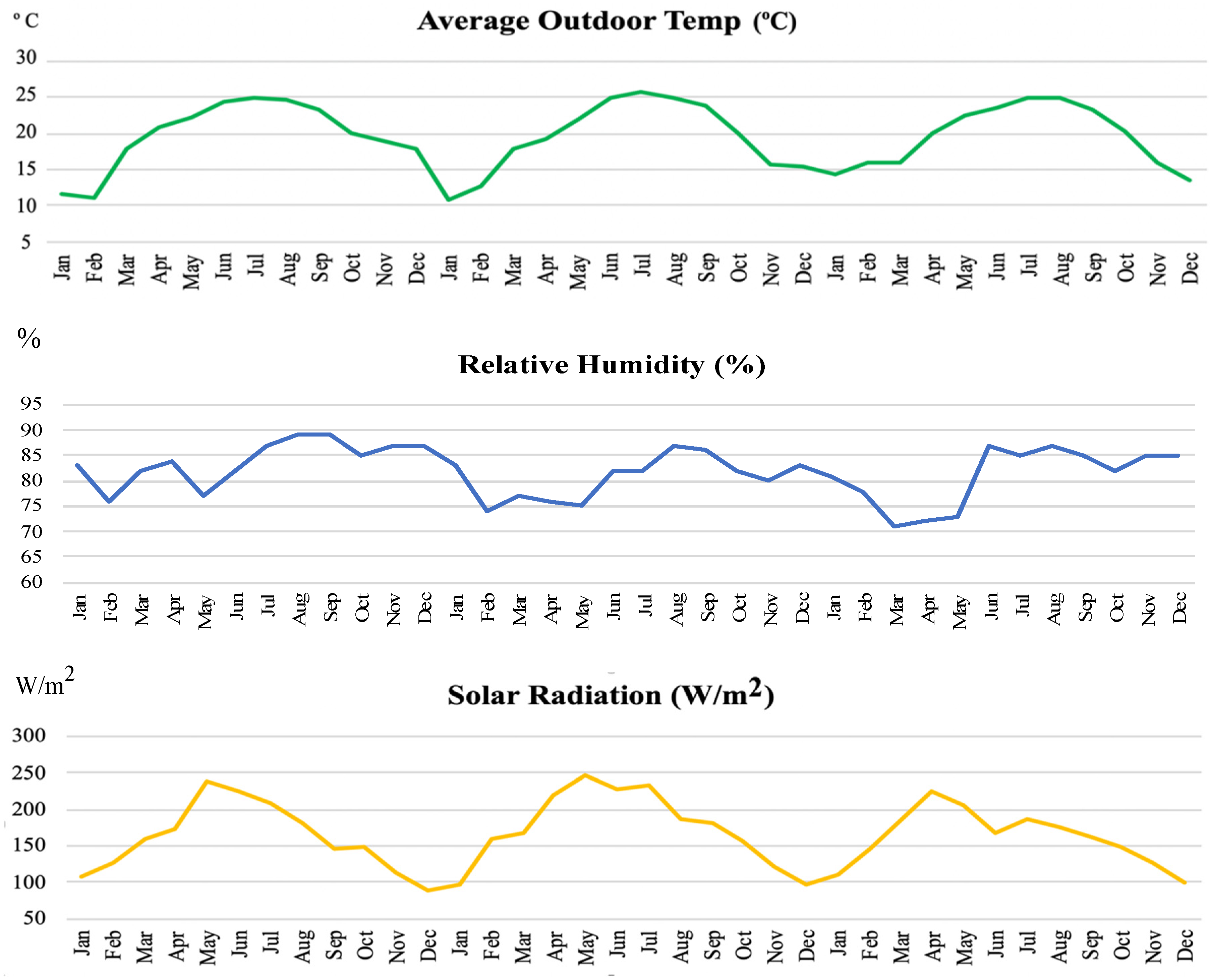
(D) Monthly and hourly average outdoor temperatures (°C), relative humidity (%), and solar radiation (W/m²) for UF campus were collected from the Florida Automated Weather Network (FAWN) and can be seen in Figure 2. In addition, in order to assess the effects of climate change on campus energy consumption, we collected hourly average outdoor temperatures (°C), relative humidity (%), and solar radiation (W/m²) for the city of Gainesville, FL for three future weather scenarios based on their impact, namely the median (year 2063), hottest (2057), and coldest (2041), representing climate conditions for the 2038 to 2066 period. The climate scenarios were created by a proprietary algorithm developed by SeventhWave, a not-for-profit company in Madison, Wisconsin. The algorithm uses climate change variables from North American Regional Climate Change Assessment Program (NARCCAP), which is an international program that serves the high-resolution climate scenario needs of the United States, Canada, and northern Mexico, and uses a regional climate model, coupled global climate model, and time-slice experiments.

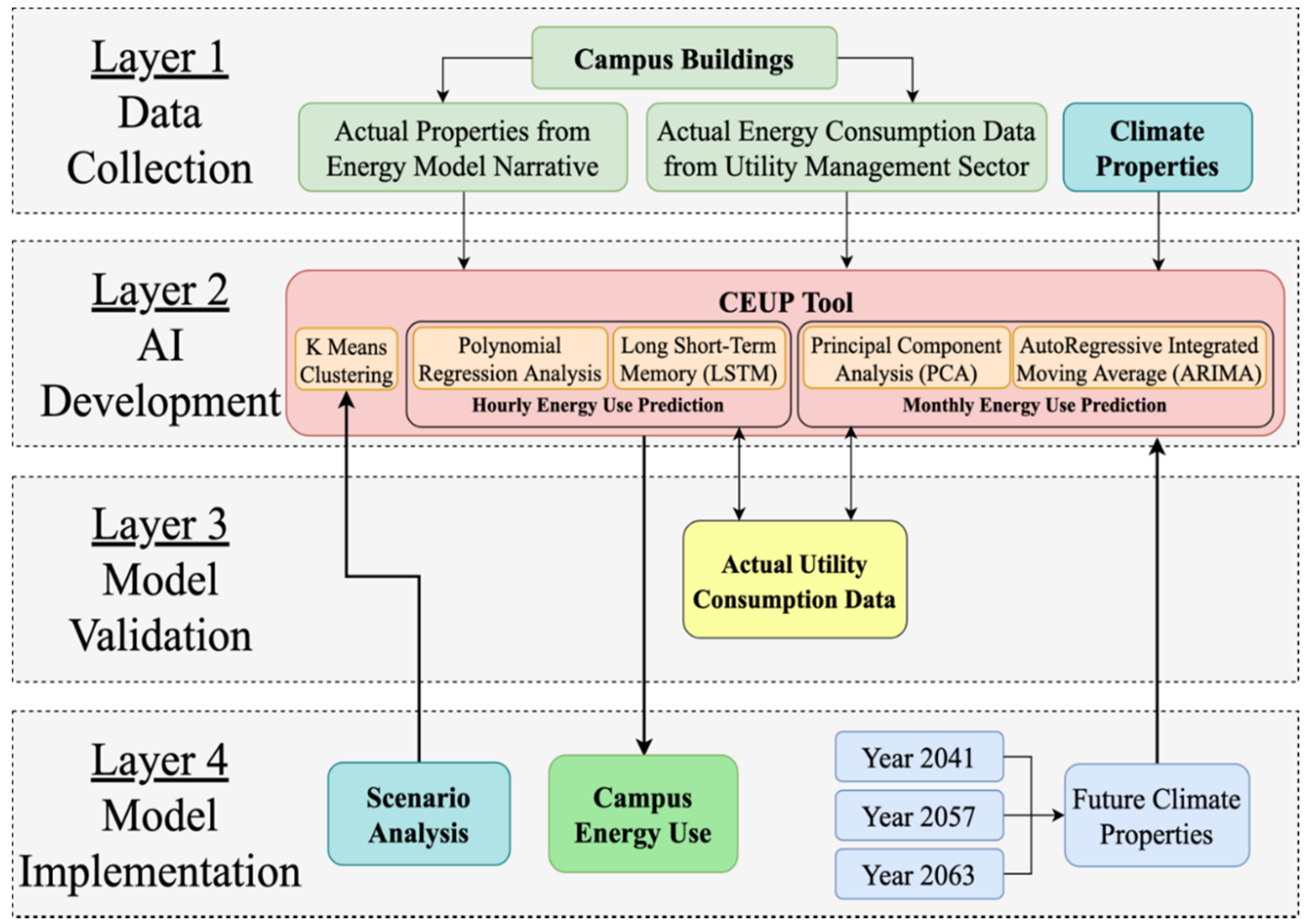
4.2. Layer 2: AI Development

This section describes how the model was developed for AI model implementation. In order to forecast the energy performance of buildings based on their historic consumption and climate data and thermophysical properties, we implemented k-means clustering, PCA, ARIMA, polynomial regression analysis, and Long Short-Term Memory (LSTM) methods.

4.2.1. K-Means Clustering

For clustering, we used eight input variables which are a linear combination of the initially introduced thermophysical and space functionality variables as follows:

• Building Thermophysical Properties: 1.1. Total U-value × Area (W/°C), 1.2. Windows SHGC × Area (m²), and 1.3. Total Power (W).
• Space Functionality Percentages: 2.1. Classroom, 2.2. Office, 2.3. Residential, 2.4. Teaching Laboratories, and 2.5. Research Laboratories.

Variable 1.1 is the sum–product of exterior walls and windows U-values and their surface areas in W/°C, variable 1.2 is the sum–product of window SHGC and their surface area in m², and variable 1.3 is building total lighting and equipment power in Watts.

The buildings were clustered into similar building types using the k-means approach to reduce the complexity of forecasting, so that there was no need to model each and every campus building in order to predict its energy consumption. Also, building clusters were used in extrapolating representative building energy use to campus energy use. K-means is usually used for cluster analysis in data mining. It aims to partition n observations into k clusters in which each observation fits to the cluster with the closest mean, that is, the cluster prototype.

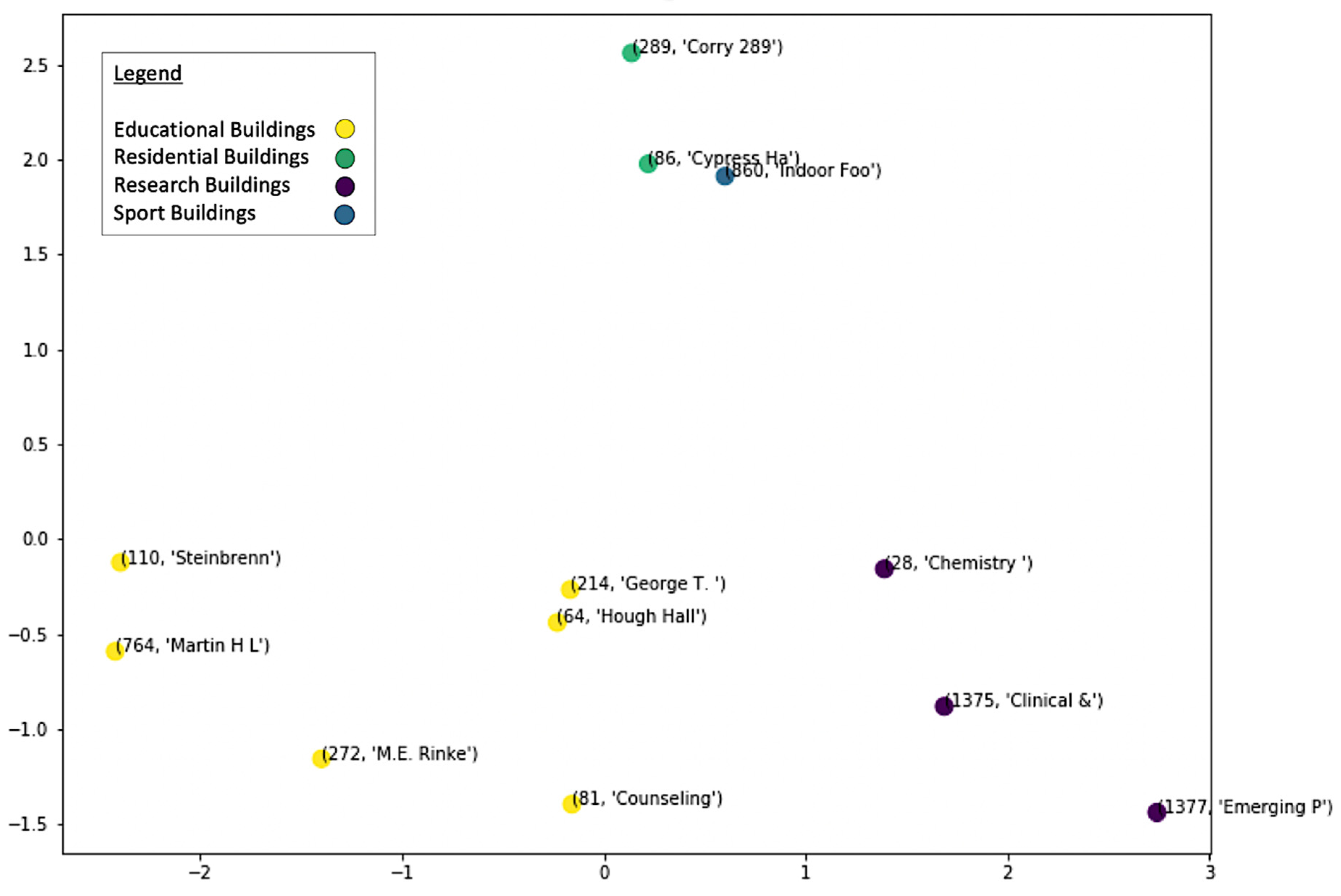
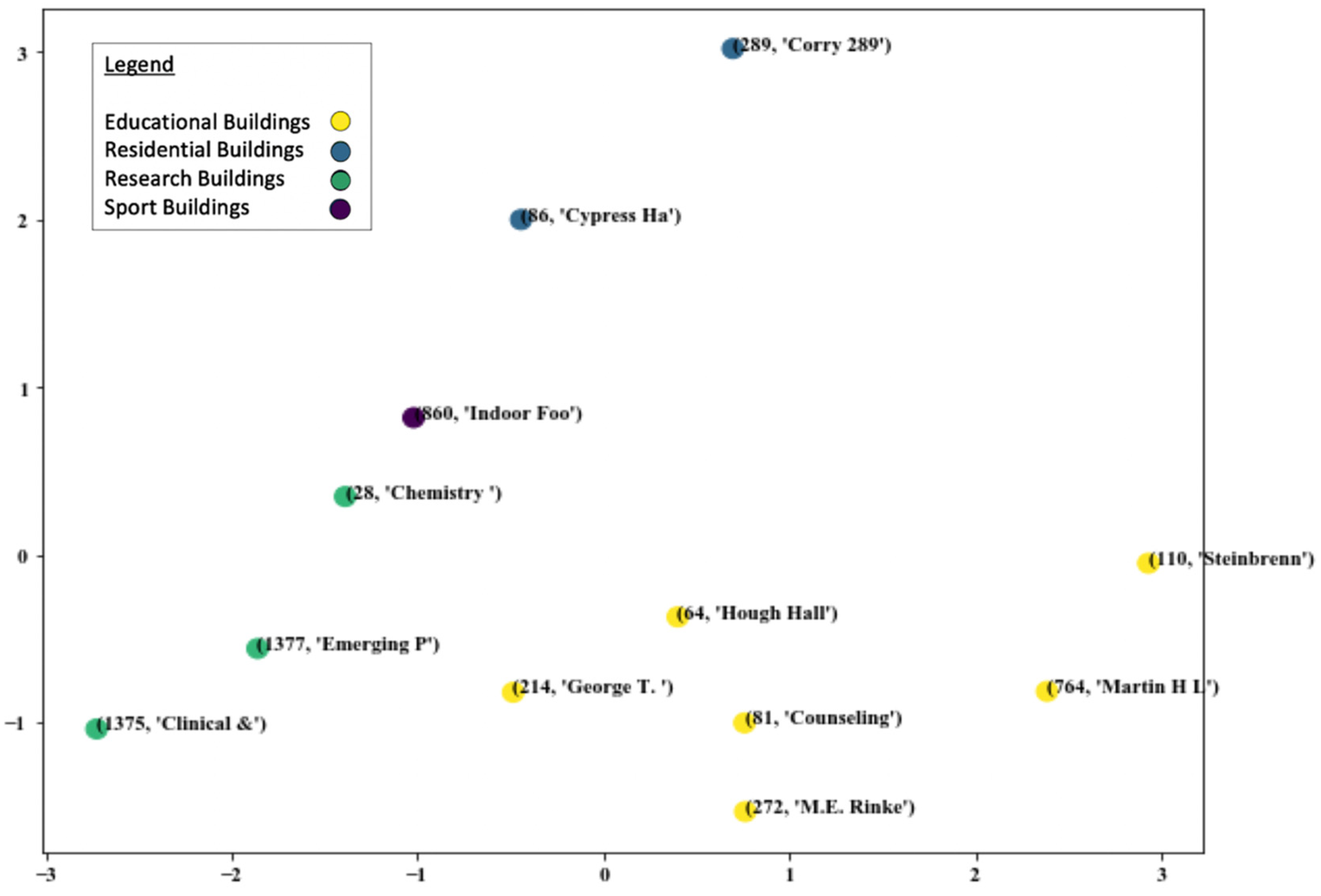
Figure 3 shows the results of clustering buildings based on their thermophysical and space functionality properties using k-means clustering. The method alternates between two steps:

• Assigning each observation to the cluster with the least-squared Euclidean distance from its mean.
• Calculating the new means of the observations in the new clusters.

Here, each axis is a unitless linear combination of the eight independent thermophysical and space functionality variables that we defined in our study. The reason for using such functions was simply that we were unable to map each of the buildings in an 8-dimensional space. Therefore, we needed to use these functions to map the buildings in a 2-dimensional space. As a result, we could partition the buildings into four clusters of educational (yellow), residential (green), research (purple), and sport (blue) buildings. We could observe that buildings with similar space functionalities and thermophysical properties are located closer to each other in the k-means clustering 2-dimensional map. Also, we see that building 0860 is located near the residential buildings, but as we knew the sport functionality of this building, we categorized it in a different cluster.

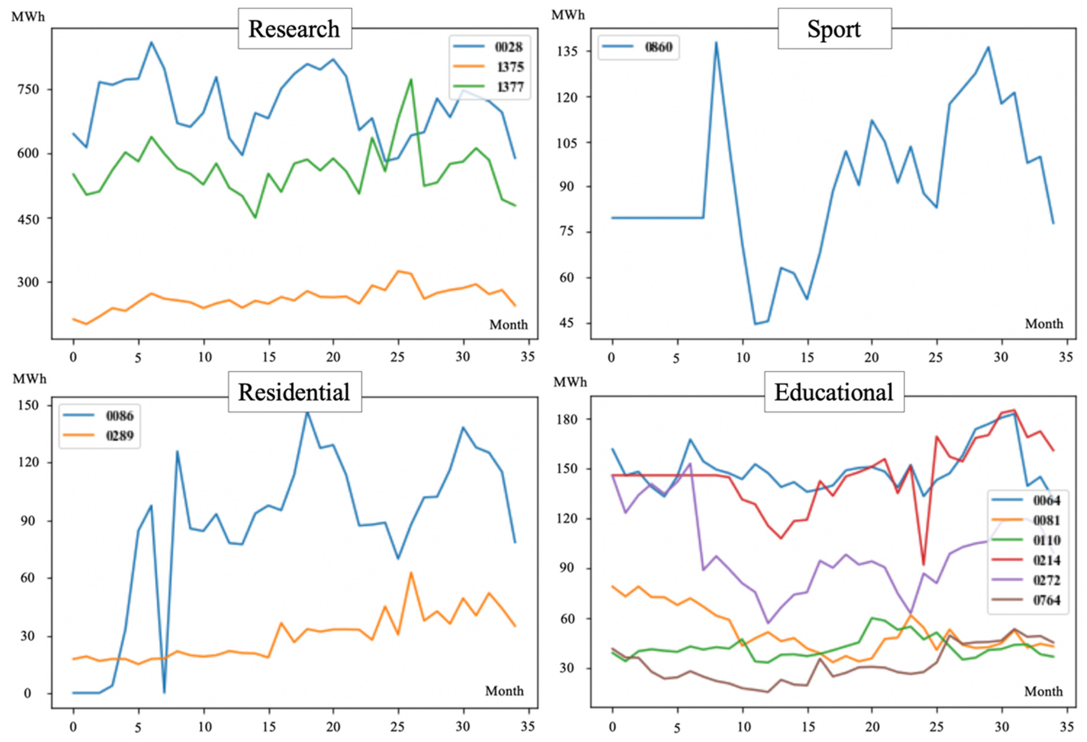
Figure 4 shows the 3-year (2015–2017) monthly energy consumption in MWh for buildings within each of the clusters. Clusters 0, 1, 2, and 3 are of type research, sport, residential, and educational buildings, respectively. The relative similarity of the consumption patterns over time for the buildings within a cluster could be observed.

4.2.2. PCA and ARIMA

PCA is a multivariate statistical approach for assessing the correlations existing among a set of intercorrelated variables. Being able to categorize a complex and highly intercorrelated set of variables, PCA gives a better understanding of cause and effect relationships. Tardioli et al. [31] used PCA, k-means clustering, and RF to identify representative buildings and building groups in a set of commercial urban buildings by using building typology, construction period, district location, building final use and geometric information. In this study, we conducted PCA in order to prioritize the eight independent variables based on their effects on campus building energy consumption.

ARIMA models are the most typical model of time series prediction methods. Lu et al. [32] used ARIMA, ANN, and SVR to predict the hourly electricity, heating, and cooling energy consumption for a set of community sports buildings, in which they considered building heterogeneity to improve forecast accuracy. Initially, ARIMA forecasting was conducted for each cluster prototype representing the average amount of energy consumption of buildings within each cluster. Here, the training size was 75% of the available data and the testing size was 25%. After training, the overall energy consumption of buildings could be forecasted using their cluster prototype for 2018. The dependent variable was the total monthly energy consumption, normalized by the average outdoor temperature in each month, in order to include the effects of this climate variable in the prediction model.

As a measure of accuracy, we used Mean Squared Error (MSE). We calculated the error percentages by dividing MSE by the cluster’s representative building energy consumption, which was the average amount of energy consumption of buildings within each cluster.

Table 3. Comparison of prediction error percentages.

Bldg. ID	MSE/Mean Percentage of Error
	Autoregressive Integrated Moving Average (ARIMA)	Principal Component Analysis (PCA) + ARIMA
0028	8.13	8.87
0064	15.60	12.16
0081	30.19	20.37
0086	19.68	17.48
0110	18.62	11.40
0214	16.29	12.66
0272	17.18	17.17
0289	13.50	10.70
0764	27.17	4.49
0860	20.12	17.64
1375	29.62	21.05
1377	8.87	6.38

shows the comparison of output errors of the forecasting results.

Based on this comparison, we concluded that for the majority of buildings, conducting PCA with ARIMA forecasting would result in better accuracy. Also, it should be noted that PCA reduces the dimension of input variables significantly and hence results in better accuracy. Consequently, in order to increase the model accuracy levels, instead of forecasting only based on cluster representative buildings, we conducted PCA and ARIMA for all the 12 buildings used in this study.

4.3. Layer 3: Model Validation

To make CEUP more reliable, we needed to validate it with the buildings’ actual energy use. The validation process was essential in order to produce realistic energy use predictions. Our validation method followed these steps:

• Compare CEUP results with the buildings’ actual energy use;
• Calculate validation measures (i.e., RMSE, etc.);
• Compare the validation measures to the allowable range according to building energy codes.

For validation of CEUP monthly energy forecasting, according to availability of actual energy consumption data, we used the buildings’ monthly energy consumption data from year 2017. As an example, Figure 5 shows actual versus CEUP simulated energy use for the educational cluster representative, UF Rinker School of Construction Management. Other than the month of February, the actual versus CEUP simulated energy consumption patterns were quite similar. The inconsistency can by due to energy sensor malfunction in that specific month.

Referring to the American Society of Heating, Refrigerating and Air-Conditioning Engineers (ASHRAE) guidelines, the acceptable range of CVRMSE for monthly validation is ±15%.

Table 4. CVRMSE for actual vs. CEUP results in MWh for Rinker Hall, the educational cluster representative.

	Actual	CEUP
Jan	85.95	98.45
Feb	79.23	113.69
Mar	96.38	97.28
Apr	100.35	109.59
May	102.43	115.16
Jun	103.67	113.40
Jul	115.13	123.07
Aug	116.71	119.84
Sept	116.66	135.38
Oct	112.69	127.17
Nov	97.07	102.55
Dec	85.42	78.52
	CVRMSE	14.1%

shows the CVRMSE calculations for actual energy use versus CEUP simulations for Rinker Hall. The calculated 14.1% CVRMSE is within the acceptable ranges of ASHRAE code.

Accordingly, the CVRMSE for actual energy use versus CEUP simulations for research, sport, and residential cluster representative buildings were calculated as 9.22%, 8.3%, and 9.13%, meeting ASHRAE requirements and validating CEUP acceptable levels of accuracy.

4.4. Layer 4: Model Implementation

4.4.1. Hourly Energy Use Prediction Based on Climate and Temporal Properties

In order to predict the energy use of campus buildings in hourly time intervals, and regarding data availability, we collected hourly utility consumption data for eight of the sample buildings used in this study for two years between January 2016 to December 2017 (dependent variables). In addition, average outdoor temperature (°C), relative humidity (%), and solar radiation (W/m²) values were collected for the two years of study, as well as the three years of future climate scenarios for the years 2041, 2057, and 2063. Furthermore, to account for the effects of seasonality, we introduced hour of day as the temporal variable (independent variables). Also, we have considered the absolute deviation of average outdoor temperature and cooling degree days baseline (Tcdd, 18.3 °C) and its squared values as two other independent variables for our study. In order to predict a campus building’s hourly energy use, we assessed the performance of two methods that we describe in the following sections.

Polynomial Regression Analysis

Initially, we calculated the correlation coefficients between the buildings’ energy use and the four climatic and temporal predictive variables for hourly values, which can be found in

Table 5. Correlation coefficients between dependent and independent variables for hourly energy consumption values.

	Hour of Day	T.Avg	T.Cdd	Sq T.Cdd	Rel. Hum.	Sol. Rad.	Bldg. 0064	Bldg. 0081	Bldg. 0110	Bldg. 0272	Bldg. 0764	Bldg. 0028	Bldg. 1375	Bldg. 1377
Hour of Day	1	0.23	0.06	0.04	−0.35	0.06	0.28	0.01	0.29	0.00	0.07	−0.14	0.16	0.06
T.Avg	0.23	1	0.16	0.10	−0.34	0.53	0.73	−0.14	0.17	−0.04	0.62	−0.69	0.82	0.81
T.Cdd	0.06	0.16	1	0.96	−0.35	0.42	0.30	0.00	0.11	0.02	0.35	0.11	0.34	0.23
Sq T.Cdd	0.04	0.10	0.96	1	−0.34	0.39	0.24	0.01	0.08	0.02	0.31	0.17	0.28	0.18
Rel. Hum.	−0.35	−0.34	−0.35	−0.34	1	−0.61	−0.22	−0.16	−0.20	−0.03	−0.30	0.02	−0.25	0.00
Sol. Rad.	0.06	0.53	0.42	0.39	−0.61	1	0.44	0.18	0.29	0.00	0.49	−0.18	0.52	0.36
Bldg. 0064	0.28	0.73	0.30	0.24	−0.22	0.44	1	−0.02	0.26	−0.01	0.73	−0.48	0.73	0.73
Bldg. 0081	0.01	−0.14	0.00	0.01	−0.16	0.18	−0.02	1	0.13	0.01	0.06	0.20	−0.11	−0.16
Bldg. 0110	0.29	0.17	0.11	0.08	−0.20	0.29	0.26	0.13	1	0.00	0.20	−-0.04	0.19	0.06
Bldg. 0272	0.00	−0.04	0.02	0.02	−0.03	0.00	−0.01	0.01	0.00	1	0.00	0.06	−0.02	−0.03
Bldg. 0764	0.07	0.62	0.35	0.31	−0.30	0.49	0.73	0.06	0.20	0.00	1	−0.35	0.66	0.61
Bldg. 0028	-0.14	−0.69	0.11	0.17	0.02	−0.18	−0.48	0.20	−0.04	0.06	−0.35	1	−0.56	−0.59
Bldg. 1375	0.16	0.82	0.34	0.28	−0.25	0.52	0.73	−0.11	0.19	−0.02	0.66	−0.56	1	0.84
Bldg. 1377	0.06	0.81	0.23	0.18	0.00	0.36	0.73	−0.16	0.06	−0.03	0.61	−0.59	0.84	1

. The correlations between the buildings’ hourly energy consumptions and average outdoor temperature was considerably higher than the other two climatic variables and the temporal variable. This shows that among climatic and temporal variables, average outdoor temperature is a better measure to predict hourly energy consumption of campus buildings given the available consumption data. Then, we conducted regression analysis to assess the performance of the four variables in predicting the buildings’ hourly energy consumption. Six degrees of regression were tested for the prediction variables. R-squared values which are statistical measures of how close the data are to the fitted regression line, were calculated for each degree of regression analysis.

As it can be seen in

Table 6. R-squared values of various degrees of polynomial regression analysis of the buildings’ hourly energy use.

Building	Polynomial Regression Degrees
	1	2	3	4	5	6
Bldg. 0064	0.598	0.782	0.823	0.837	0.855	0.859
Bldg. 0081	0.135	0.283	0.325	0.366	0.395	0.426
Bldg. 0110	0.172	0.295	0.381	0.407	0.436	0.451
Bldg. 0272	0.004	0.009	0.013	0.021	0.032	0.047
Bldg. 0764	0.465	0.689	0.737	0.774	0.789	0.783
Bldg. 0028	0.559	0.612	0.620	0.627	0.636	0.647
Bldg. 1375	0.737	0.767	0.776	0.783	0.789	0.792
Bldg. 1377	0.777	0.850	0.856	0.861	0.865	0.867

, as we increased the polynomial degrees, the R-squared values tended to increase, toward higher accuracy of fitted lines. However, raising the polynomial regression degrees can result in higher chances of overfitting the regression, which we wanted to avoid. Therefore, we concluded that polynomial regression analysis is not an appropriate method for predicting hourly energy use of campus buildings over an entire year, given the amount of available data. It was expected that other models that can capture more feedbacks would perform better than regression models.

Long Short-Term Memory (LSTM)

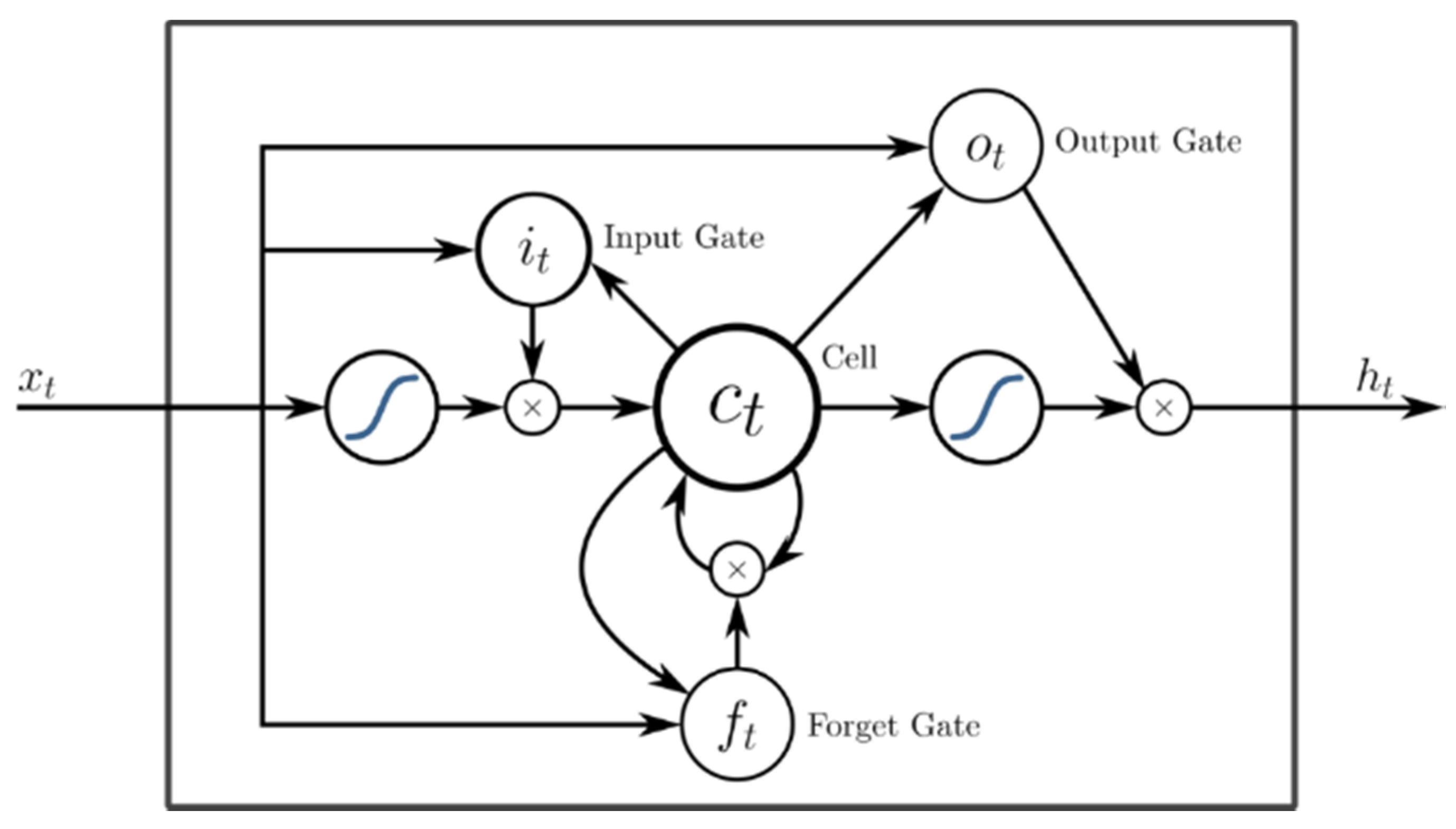
LSTM blocks are building units for layers of Recurrent Neural Networks (RNN). RNNs composed of LSTM units are usually called LSTM networks. LSTM units have various architectures. A usual LSTM unit is composed of a cell, an input gate, an output gate, and a forget gate. The cell accounts for memorizing values over random time intervals and, as a result, the memory in LSTM. The three gates can be considered as an artificial neuron, the same as a feedforward/multilayer neural network. Figure 6 shows a typical LSTM cell used to forecast time series data, where $x_t$ is the input vector for LSTM unit, $f_t$, $i_t$, and $o_t$ are the activation vectors for the forget gate, the input gate, and the output gate, $h_t$ is the output vector for the LSTM unit, and $c_t$ is the cell state vector. Average outdoor temperature, relative humidity, solar radiation, and hour of the day were used as the predictor variables in this method.

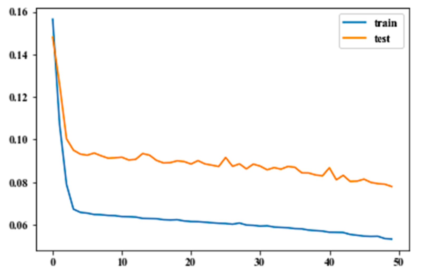
We allocated 50% of the consumption data to model training and the other 50% to model testing. Also, while training neural networks, one epoch refers to one passage of the entire training set. In this analysis, we considered 50 epochs for training and testing steps. Mean squared error was used as the objective loss function to minimize, in order to assess the accuracy levels of LSTM. As an example, Figure 7 shows the loss (unitless) values of training and testing hourly energy consumption for building 1377, Emerging Pathogens Institute, over 50 epochs. As can be seen, after 50 epochs, the error percentage of tested data was almost 8%, hence, representing the high level of LSTM accuracy for predicting the buildings’ hourly energy use based on the four climatic and temporal variables, as well as complying with the +/–15% acceptable error of the ASHRAE-14 guideline.

Accordingly, we predicted the hourly energy consumption of the eight buildings for the three climate scenarios. LSTM is a prediction method for time series data, and currently we only know the building’s consumption values as of now, and hence, there are no data from now to any of the future years for which we are interested in predicting the consumption pattern and values. As a result, the levels of error for predicting three years far in the future was relatively high. Consequently, the predicted scenario results were normalized by the mean values of consumptions over a year, in order to mitigate the effects of the induced error. As an example, Figure 8 shows the LSTM-predicted hourly energy consumption (in MWh) of building 0064, UF Hough Graduate School of Business, for the median (year 2063), hottest (2057), and coldest (2041) future scenarios.

It should be noted that, based on the nature of the LSTM prediction method, while normalizing and forecasting the hourly energy consumption values, a few negative values were observed, which were considered as 0.

4.4.2. Monthly Energy Use Prediction Based on Climate Properties

Table 7. CEUP simulated 2018 monthly energy consumption (MWh) for the twelve buildings used in the study.

Bldg. ID		0028	0064	0081	0086	0110	0214	0272	0289	0764	0860	1375	1377	Totals
Month	Tavg
2018-1	14.91	567.8	130.0	53.3	86.6	46.3	89.9	97.3	37.0	25.5	78.6	266.2	544.6	2023.1
2018-2	16.57	574.9	139.6	40.1	68.2	50.3	165.0	115.5	15.2	25.2	66.6	301.9	664.1	2226.7
2018-3	16.72	626.8	143.5	52.2	85.7	42.2	153.3	92.4	34.6	27.0	87.9	283.9	755.2	2384.5
2018-4	21.04	634.1	153.9	43.1	99.4	34.5	150.5	110.7	14.5	24.2	97.3	231.2	511.4	2104.9
2018-5	23.78	711.5	169.3	41.3	99.7	35.6	164.2	119.5	18.8	24.5	101.9	244.0	519.2	2249.5
2018-6	25.15	668.3	172.4	41.8	113.6	40.1	165.8	112.3	12.6	25.6	110.5	250.9	561.8	2275.7
2018-7	26.57	730.2	176.0	44.1	135.0	40.7	178.8	127.3	25.7	25.8	92.2	255.4	566.9	2398.1
2018-8	26.63	717.4	178.3	51.7	124.8	43.2	180.5	115.8	14.9	30.4	93.9	262.1	597.7	2410.6
2018-9	24.91	705.1	136.1	41.5	122.2	43.4	164.6	138.2	27.4	27.1	72.1	240.6	570.5	2288.9
2018-10	21.57	679.5	141.5	43.7	112.4	37.6	168.1	122.4	20.5	29.2	75.1	250.9	480.4	2161.3
2018-11	16.60	575.0	128.6	42.2	76.6	36.2	156.9	102.3	7.7	23.2	49.7	211.6	466.7	1876.7
2018-12	16.02	666.3	148.4	60.5	85.5	53.8	147.7	79.7	18.7	25.7	92.6	275.6	621.7	2276.2
												12 buildings total energy use		26676

shows the CEUP simulated monthly energy consumption values in MWh for the twelve buildings used in this study by using the ARIMA forecasting technique. The total energy consumption, normalized by average outdoor temperature values, was simulated with the CEUP tool for year 2018 and was calculated to be 26,676 MWh for the twelve buildings. According to the utility consumption data from UF PPD, we could extrapolate the consumption of this set of buildings to the entire UF campus, based on campus buildings space functionality percentages, and predict 2018 campus energy consumption to be 812,560 MWh.

4.4.3. Extrapolation to Campus Energy Consumption

We calculated UF campus buildings’ energy consumption by extrapolating the consumption of the set of representative buildings to the entire UF campus, based on campus buildings’ space functionality percentages. According to US NARCCAP future climate scenarios, in order to estimate campus operational energy consumption under long-term climate change, three future climate scenarios, median, hottest, and coldest annual average temperature, were used. Considering year 2018 as the simulation baseline, with the mentioned approaches for hourly and monthly CEUP, we predicted annual campus energy consumption values for the three future climate scenarios. The results in MWh can be found in

Table 8. Campus energy use and average outdoor temperature for baseline and future climate scenarios.

	Actual	CEUP Simulation
Year	2018	2018	2041	2063	2057
Scenario	Baseline	CEUP	Coldest	Median	Hottest
Avg. Outdoor Temp. (°C)	21.17	21.17	19.82	22.18	20.99
Campus Energy Demand (MWh)	752,858	812,560	780,262	901,999	838,458
Percentage Difference		7.93%	+3.64%	+11.37%	+19.81%

.

It can be seen that the variation of campus energy use in the upcoming 40 years, based on NARCCAP future weather scenarios, can be between +3.64% to +19.81%, and should be managed accordingly. CEUP is a credible tool for predicting campus energy use, and given various possible climate scenarios, CEUP can be helpful to campus energy managers to plan their energy strategies. Also, by using additional building data, we can increase the forecasting accuracy levels and develop the CEUP model to be representative of campus energy performance.

4.4.4. Scenario Analysis

After calculating the campus energy use for the three future scenarios, we wanted to assess how the changes in building thermophysical properties would change the campus energy consumption in the three future scenarios of the median (year 2063), hottest (2057), and coldest (2041). In order to conduct this analysis, we referred to the technology roadmap that is used to assess and present the development of technology products in building sector. The technology roadmap for building sectors can be categorized into five groups: building envelope, lighting, electronics, HVAC, and energy management, among which our focus is on the building envelope group. According to the Technology Roadmap—Energy Efficient Building Envelopes (IEA, 2013), we introduced five envelope scenarios for each of the future climate scenarios, as can be seen in

Table 9. Five envelope future scenarios based on Technology Roadmap, International Energy Agency (IEA), 2013 [30].

Envelope Scenario	Envelope Properties	Future Climate Scenario
		2041	2063	2057
		Coldest	Median	Hottest
1	Wall U-Value (W/m2 °C)	0.24	0.18	0.19
2	Roof U-Value (W/m2 °C)	1.99	1.99	1.99
3	Windows U-Value (W/m2 °C)	4.26	4.26	4.26
4	Windows SHGC	0.2	0.2	0.2
5	1 to 4 Combined	All Above	All Above	All Above

.

By updating CEUP results according to the properties of five envelope scenarios, the configurations of building clusters change, resulting in different campus energy use predictions for the three future climate scenarios. As an example, Figure 9 shows the updated building k-means clustering result for envelope scenario 5.

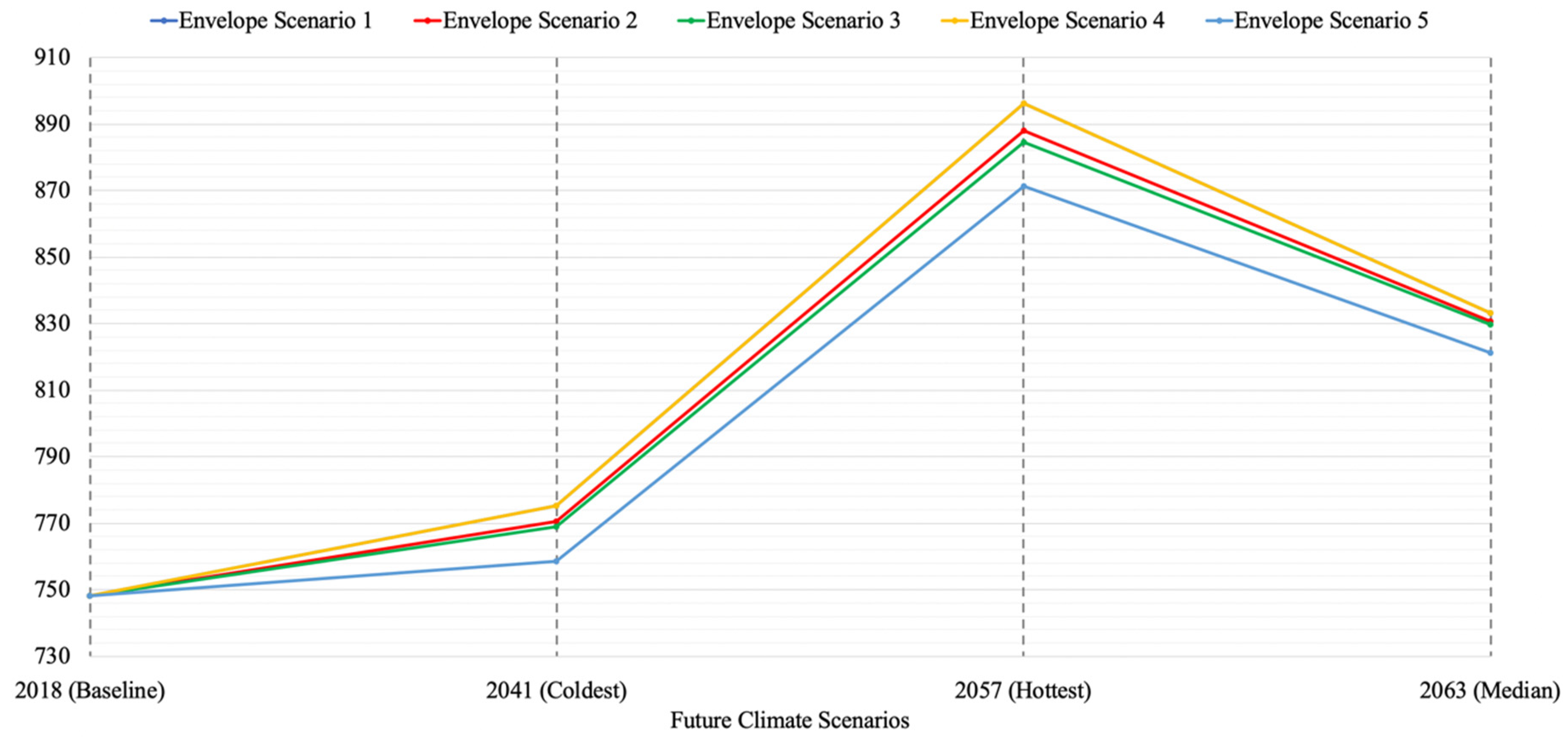
According to the updated building clustering, CEUP simulation results for the future climate and envelope scenarios can be seen in Figure 10 and

Table 10. CEUP simulation results for the future climate and envelope scenarios.

Envelope Scenario	CEUP for Future Climate Scenario (MWh)
	2041	Difference with 2018 Baseline (%)	2063	Difference with 2018 Baseline (%)	2057	Difference with 2018 Baseline (%)
	Coldest		Median		Hottest
1	775.36	3.64	833.19	11.37	896.33	19.81
2	770.42	2.98	830.57	11.02	887.87	18.68
3	768.85	2.77	829.74	10.91	884.51	18.23
4	775.36	3.64	833.19	11.37	896.33	19.81
5	758.52	1.39	821.14	9.76	871.19	16.45

. In all envelope scenarios, campus energy consumption rises when compared to the baseline year of 2018. It should be noted that the highest energy use level happens in year 2057 (hottest climate scenario).

According to the scenario analysis results, we could observe that scenario 5 had the most influence on campus energy use when compared to the other scenarios. According to this scenario, campus energy use can be between 1.39% to 16.45% higher when compared to the amount of energy used by the campus in the baseline year 2018, for the three future climate scenarios.

5. Conclusions

This study developed a data-driven, campus-scale energy use prediction, which implemented artificial intelligence in order to assess the effects of long-term climate change. Our study consisted of four layers: (1) Data Collection, (2) AI Development, (3) Model Validation, and (4) Model Implementation. We relied on energy use data for buildings at the University of Florida, Gainesville, FL. To study the impact of climate change, we used average outdoor temperature, solar radiation, and relative humidity of three future climate weather files of Gainesville, FL, represented and based on their impact: median (year 2063), hottest (2057), and coldest (2041). In order to conduct the scenario analysis, we referred to the Technology Roadmap—Energy Efficient Building Envelopes (IEA 2013), which is used to assess and present the development of technology products in the building sector. According to the roadmap, we assessed campus energy use for five envelope scenarios for each of the future climate scenarios.

In this study, we used space functionality characteristics of various buildings in relatively accurate gross square foot percentages as inputs to our prediction model. This approach is unique to its kind and has not been used in other data-driven, urban level building energy prediction studies. According to our results:

• CEUP model can predict the energy use of campus buildings with 90% accuracy.
• UF campus energy use in the upcoming 40 years, based on NARCCAP future weather scenarios, can be up to 20% higher.
• Among climatic and temporal variables, average outdoor temperature is a good measure to predict hourly energy consumption of campus buildings.
• Incorporating building functionalities in space-level can increase the accuracy of physics-based building clustering and hence result in better prediction accuracy.

CEUP can be a useful tool in predicting residential and commercial buildings’ energy consumption with more accuracy, and therefore also predict the aggregate energy consumption for urban areas as well. Given that, CEUP has the potential to be updated with additional buildings and incorporate various climate variables in order to be used as a comprehensive decision-making tool for city and community managers. Also, new buildings which are going be added to the community can be designed based on optimized building specifications, in order to better participate in the reduction of building environmental footprints. Therefore, CEUP can be both a decision making and sustainable design tool helpful to building architects as well.

The next steps are to obtain more building data as well as introduce more independent variables to increase the accuracy levels of the model. As more building data are collected and analyzed, other building characteristics such as HVAC specifications can be incorporated into the model to improve its prediction accuracy. In addition, shifting the modeling time intervals to subhourly and near real-time levels can improve accuracy. Furthermore, as the number of buildings is increased, it is likely that the number of clusters will also increase, expanding the range of building functionality types within campuses, communities, and cities. Such modifications can help in improving the level of accuracy and provide a more accurate building energy use prediction under various climate scenarios.

References

1. Melillo, J.M. Climate Change Impacts in the United States: The Third National Climate Assessment; Government Printing Office: Washington, DC, USA, 2014.
2. Intergovernmental Panel on Climate Change (IPCC). United Nations Body for Assessing the Science Related to Climate Change; IPCC: Geneva, Switzerland, 2018.
3. United States Energy Information Administration (EIA). International Energy Outlook 2017. Available online: https://www.eia.gov/outlooks/archive/ieo17/ (accessed on 4 October 2018).
4. International Energy Agency (IEA). Energy consumption by sector. Available online: http://www.eia.doe.gov/emeu/aer/pdf/pages/sec2.pdf (accessed on 4 October 2018).
5. Hill, M.C.; Banta, E.R.; Harbaugh, A.W.; Anderman, E.R. MODFLOW-2000, the US Geological Survey Modular Ground-Water Model; User Guide to the Observation, Sensitivity, and Parameter-Estimation Processes and Three post-Processing Programs; No. 2000-184; US Geological Survey: Virginia Reston, VA, USA, 2000.
6. EPBD Directive 2002/91/EC. Directive of the European parliament and of the council on the energy performance of buildings. Eur. Commun. Off. J. 2003, L001, 65–71. Available online: https://eur-lex.europa.eu/LexUriServ/LexUriServ.do?uri=OJ:L:2003:001:0065:0071:EN:PDF (accessed on 4 October 2018).
7. Kibert, C.J. Sustainable Construction: Green Building Design and Delivery; John Wiley & Sons: Hoboken, NJ, USA, 2016. [Google Scholar]
8. International Energy Agency (IEA). Global Engagement, United Kingdom. Available online: https://www.iea.org/countries/United%20Kingdom/ (accessed on 4 October 2018).
9. Committee on Climate Change (CCC), Independent advice to government on building a low-carbon economy and preparing for climate change. Available online: https://www.theccc.org.uk/ (accessed on 13 May 2017).
10. Perez-Lombard, L.; Ortiz, J.; Pout, C. A review on buildings energy consumption information. Energy Build. 2018, 40, 394–398. [Google Scholar] [CrossRef]
11. United Nations DESA Population Division. World Population Prospects. 2017. Available online: https://population.un.org/wpp/ (accessed on 6 December 2018).
12. City of New York. One City Built to Last; Mayor’s Office of Long-Term Planning and Sustainability: New York, NY, USA, 2014. [Google Scholar]
13. Greenovate Boston. 2014 Climate Action Plan Update; Greenovate Boston: Boston, MA, USA, 2014. [Google Scholar]
14. Song, H.; Srinivasan, R.; Jeschke, S.; Sookoor, T. Smart Cities: Foundations, Principles and Applications; John Wiley & Sons: Hoboken, NJ, USA, 2017. [Google Scholar]
15. Cajot, S.; Peter, M.; Bahu, J.M.; Guignet, F.; Koch, A.; Maréchal, F. Obstacles in energy planning at the urban scale. Sustain. Cities Soc. 2017, 30, 223–236. [Google Scholar] [CrossRef]
16. Berardi, U. A cross-country comparison of the building energy consumptions and trends. Resour. Conserv. Recycl. 2017, 123, 230–241. [Google Scholar] [CrossRef]
17. Al-Homoud, M.S. Computer-aided building energy analysis techniques. Build. Environ. 2001, 36.4, 421–433. [Google Scholar] [CrossRef]
18. Hong, T.; Luo, X. Modeling Building Energy Performance in Urban Context. In Proceedings of the Building Performance Analysis Conference and SimBuild co-organized by ASHRAE and IBPSA-USA, Chicago, IL, USA, 26–28 September 2018. [Google Scholar]
19. Deb, C.; Zhang, F.; Yang, J.; Lee, S.E.; Shah, K.W. A review on time series forecasting techniques for building energy consumption. Renew. Sustain. Energy Rev. 2017, 74, 902–924. [Google Scholar] [CrossRef]
20. Ostergard, T.; Jensen, R.L.; Maagaard, S.E. A comparison of six metamodeling techniques applied to building performance simulations. Appl. Energy 2018, 211, 89–103. [Google Scholar] [CrossRef]
21. Reinhart, C.F.; Davila, C.C. Urban building energy modeling – A review of a nascent field. Build. Environ. 2016, 97, 196–202. [Google Scholar] [CrossRef] [Green Version]
22. Wang, Z.; Srinivasan, R.S. A review of artificial intelligence based building energy use prediction: Contrasting the capabilities of individual and ensemble prediction models. Renew. Sustain. Energy Rev. 2017, 75, 796–808. [Google Scholar] [CrossRef]
23. Neto, A.H.; Fiorelli, F.A.S. Comparison between detailed model simulation and artificial neural network for forecasting building energy consumption. Energy Build. 2018, 40, 2169–2176. [Google Scholar] [CrossRef]
24. Fathi, S.; Srinivasan, R.S.; Ries, R. Campus energy use prediction (CEUP) using artificial intelligence (AI) to study climate change impacts. In Proceedings of the 2019 Building Simulation Conference, IBPSA, Rome, Italy, 2–4 September 2019. [Google Scholar]
25. Robert, C. Machine Learning, a Probabilistic Perspective; MIT press: Cambridge, MA, USA, 2014; pp. 62–63. [Google Scholar]
26. Eisenhower, B.; O’Neill, Z.; Narayanan, S.; Fonoberov, V.A.; Mezić, I. A methodology for meta-model based optimization in building energy models. Energy Build. 2012, 47, 292–301. [Google Scholar] [CrossRef]
27. Eisenhower, B.; O’Neill, Z.; Narayanan, S.; Fonoberov, V.A.; Mezić, I. Building cooling load prediction based on time series method and neural networks. Int. J. Grid Distr. Comput. 2015, 47, 1386–1390. [Google Scholar]
28. Fathi, S.; Srinivasan, R.S.; Fenner, A. Machine learning applications in urban building energy performance forecasting: A systematic review. Renew. Sustain. Energy Rev. 2019, (in press). [Google Scholar]
29. Fathi, S.; Srinivasan, R.S. Analysis of energy performance of university campus buildings using statistical and energy modeling approaches. In Proceedings of the 2015 Winter Simulation Conference, Huntington Beach, CA, USA, 6–9 December 2015; IEEE Press: River Street Hoboken, NJ, USA. [Google Scholar]
30. Marc LaFrance. Technology Roadmap: Energy Efficient Building Envelopes; IEA: Paris, France, 2013.
31. Tardioli, G.; Kerrigan, R.; Oates, M.; O’Donnell, J.; Finn, D.P. Identification of representative buildings and building groups in urban datasets using a novel pre-processing, classification, clustering and predictive modelling approach. Build. Environ. 2018, 140, 90–106. [Google Scholar] [CrossRef]
32. Lü, X.; Lu, T.; Kibert, C.J.; Viljanen, M. Modeling and forecasting energy consumption for heterogeneous buildings using a physical–statistical approach. Appl. Energy 2015, 144, 261–275. [Google Scholar] [CrossRef]
33. Greff, K.; Srivastava, R.K.; Koutník, J.; Steunebrink, B.R.; Schmidhuber, J. LSTM: A Search Space Odyssey. IEEE Trans. Neural Netw. Learn. Syst. 2017, 28, 2222–2232. [Google Scholar] [CrossRef] [PubMed] [Green Version]
Figure 1. Model development layers for AI-based campus energy use prediction.
Sustainability 12 03223 g001
Figure 2. Average outdoor temperature (°C), relative humidity (%), and solar radiation (W/m2) at the University of Florida (UF) for January 2015 to December 2017.
Sustainability 12 03223 g002
Figure 3. Building clustering using their thermophysical and space functionality properties.
Sustainability 12 03223 g003
Figure 4. 2015–2017 monthly energy consumption in MWh for buildings within each cluster.
Sustainability 12 03223 g004
Figure 5. Actual versus Campus Energy Use Prediction (CEUP) simulated energy.
Sustainability 12 03223 g005
Figure 6. Common Long Short-Term Memory (LSTM) cell architecture [33]; x t is the input vector for LSTM unit, f t ,   i t , and o t are the activation vectors for the forget gate, the input gate, and the output gate, h t is the output vector for the LSTM unit, and c t is the cell state vector.
Sustainability 12 03223 g006
Figure 7. Loss values of train and test over 50 epochs for Building 1377.
Sustainability 12 03223 g007
Figure 8. LSTM-predicted hourly energy consumption (in MWh) of building 0064, Hough Hall, for the median (year 2063), hottest (2057), and coldest (2041) future scenarios.
Sustainability 12 03223 g008
Figure 9. Updated building clustering for envelope scenario 5.
Sustainability 12 03223 g009
Figure 10. Forecasted campus energy use under various future climate and envelope scenarios.
Sustainability 12 03223 g010