Artificial Neural Network-Based Residential Energy Consumption Prediction Models Considering Residential Building Information and User Features in South Korea

Abstract

When researching the energy consumption of residential buildings, it is becoming increasingly important to consider how residents use energy. With the advancement of computing power and data analysis techniques, it is now possible to analyze user information using big data techniques. Here, we endeavored to integrate user information with the physical characteristics of residential buildings to analyze how these elements impact energy consumption. Regression analysis was conducted to accurately identify the impact of each element on energy consumption. It was found that six elements were influential in all seasons: the number of exterior walls, housing direction, housing area, number of years occupied, number of household members, and the occupation of the household head. The elements that had an impact in each period were then derived. Based on the results of the regression analysis, input variables for the training of an artificial neural network (ANN) model were selected for each period, and residential energy consumption prediction models were implemented based on actual consumption. The elements identified as those affecting energy consumption, through regression analysis, can be used for implementing prediction models with advanced forms. This study is significant in that we derived influential elements from an integrative perspective.

1. Introduction

In 2019, the World Green Building Council reported that the energy used by buildings accounted for 30% of the world’s total energy consumption, with residential buildings representing the highest proportion (22%) [1]. The figures are similar for South Korea; the residential sector represents 17.1% of total energy consumption, with electric energy being responsible for 38.8%. This demonstrates the necessity of preparing energy-saving measures for residential buildings [2].

To reduce energy consumption in buildings, various systems for managing energy have been introduced (e.g., the building energy management system (BEMS)), and energy-saving measures have been prepared (e.g., improving physical performances related to building energy). In South Korea, such energy-saving measures and their application scope have been gradually expanded to residential buildings. In residential buildings, energy consumption is significantly affected by the attributes or sociology of the inhabitants, as well as the performance of the building. Therefore, the importance of researching energy saving using user information is increasing [3]. Moreover, it is necessary to effectively conduct sustainable energy utilization by preparing an energy reduction plan that considers user features.

Thus far, research on how the physical environment affects energy consumption has been intensively conducted; however, it is difficult to collect a large amount of user information owing to its personal nature. It is also difficult to quantitatively reduce and analyze the information on individuals. Nevertheless, the analysis of qualitative data has become possible through national surveys and new methodologies that are capable of nonlinear analysis, such as artificial neural networks (ANNs). In this study, the energy consumption in residential buildings in South Korea was investigated, by integrating the physical characteristics of residential buildings with information on occupant behavior and characteristics, to identify elements that affect residential energy consumption. The elements that were found to be influential were subsequently used to construct energy consumption prediction models.

2. Literature Review

Most studies on the energy consumption of residential buildings have focused on physical characteristics, and those that considered user behavior only considered one or two user elements. However, user information cannot be defined with such few elements; therefore, studies that reflect user information from various perspectives are required. In this study, elements that affect energy consumption were derived considering both the physical characteristics of buildings and user information.

2.1. Effects of Physical Building Characteristics on Energy Consumption

Kim [4] reported that annual power consumption varied depending on the housing type, construction year, number of floors, building structure, and building location. It was found that detached houses with relatively less energy-related facilities consumed more energy than apartments, as did old buildings and those with fewer floors. Kim et al. [5] discovered that the residential area, heating method, number of floors, and building direction all affected heating energy consumption for 181 apartment complexes in Seoul. Similarly, Eum et al. [6] reported that the construction year, household area, building direction, and heating method affected energy consumption in 21 apartment complexes in Daegu, which is located in central South Korea. In another region in central South Korea—Gyeongbuk—Lee and Chae [7] proposed that the main elements affecting energy consumption were the heating method and exterior walls and windows.

2.2. Effects of User Sociology on Energy Consumption

Van den Brom et al. [8] analyzed the actual energy consumption data of 14,000 households to examine how user features affect energy consumption. Schipper et al. [9] and Noh [10] mentioned that the relationship between energy consumption and users varies because the method and pattern of using energy are different depending on a user’s sociology [9,11].

Kim and An [12] considered the types of Korean users and reported that energy consumption was higher as income increased, because users with higher income were more sensitive to changes in their surroundings. Conversely, the energy consumption of users with relatively lower income was more affected by the physical attributes of their buildings, such as building age, than by changes in their surroundings [9].

In residential spaces, energy consumption varies depending on the residence time and lifestyle of household members. Kim et al. [5] proposed that the occupation, type of household members, and number of household members were influential elements [8]. In the case of occupation, office workers consumed more energy than the self-employed. In addition, members with longer residence times consumed more power [13].

Seo et al. [14] reported that power consumption tendency differed depending on the occupants’ income level and the type of residents. Single-person households and families without children consumed less energy, because they were socially and economically more active and thus spent less time in their houses. However, energy consumption increased upon childbirth, when their residence time and economic activity patterns changed [15].

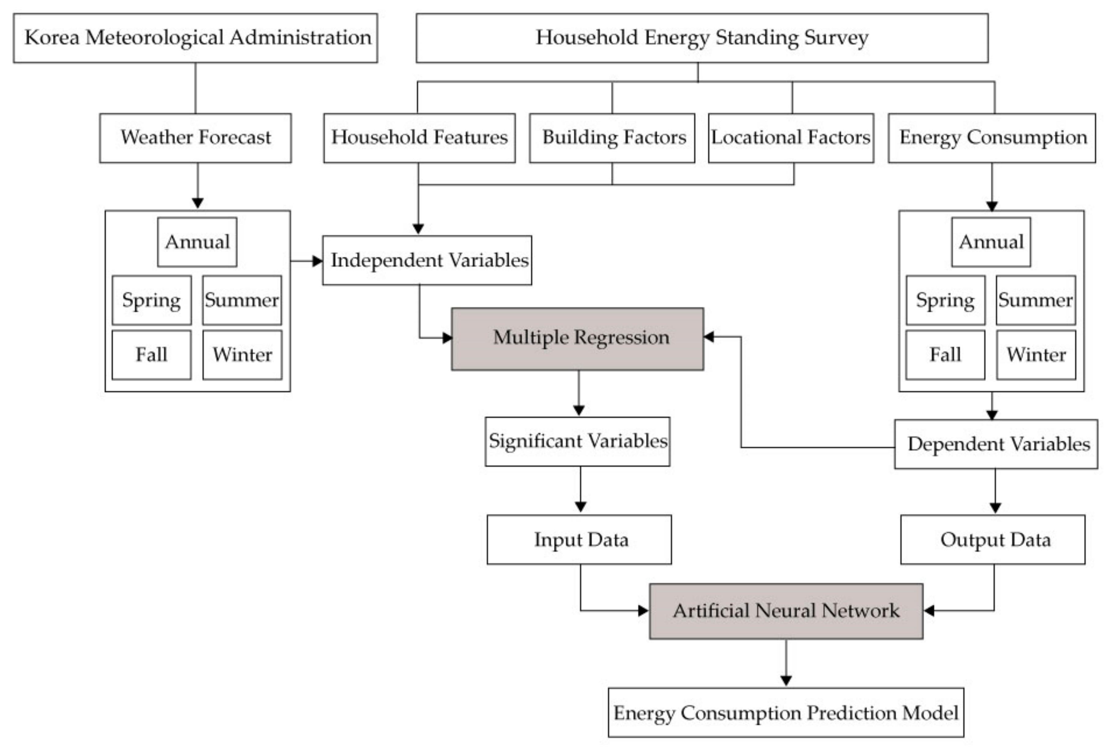
3. Materials and Methods

Figure 1 shows the research process of this study. First, data from the Household Energy Standing Survey were integrated with the annual regional temperature data of the Korea Meteorological Administration. Second, multiple regression analysis was conducted using the integrated data to obtain the elements affecting energy consumption in each season. Elements found to be influential were then used as input data to construct an ANN model and implement energy consumption prediction models. To accurately derive the elements and construct the prediction model, regression analysis and prediction model construction were conducted for five periods: spring, summer, fall, and winter, as well as annually.

3.1. Household Energy Standing Survey Data

The user data used in this study were collected from the 2016 and 2017 Household Energy Standing Survey, which is conducted annually by the Korea Energy Economics Institute. The survey respondents were from 2520 households in 16 cities and provinces and 3 metropolitan cities, with data on 19 physical housing elements, 14 heating, cooling, and cooking elements, and 14 household and household member elements. The survey also provided the monthly consumption data from 18 energy sources, including general electricity, midnight electricity, and total electricity. It was found that the earlier data were not suitable for integrating and analyzing multi-year data because of limitations in way the composition of items and code disclosure scope were recorded. Therefore, 5040 items of data from 2016 and 2017 were used in this study.

3.2. Seasonal Characteristics in South Korea and their Effects on Energy Consumption

South Korea has four distinct seasons; consequently, different home appliances and energy sources are used in each season. The seasons also affect the length of time residents spend indoors. In spring and fall, residential energy consumption is low, because there are many clear and dry days under the influence of migratory anticyclones. In summer, cooling-related energy consumption increases because the weather is hot and humid under the influence of the North Pacific anticyclone. In winter, heating-related energy consumption increases because the weather is generally cold and dry under the influence of the continental anticyclone [16].

Figure 2 shows the monthly average temperature data of 16 regions in South Korea in 2016 and 2017. In Seoul and Kyunggi-do, the cities with the highest population densities in South Korea, the average annual temperatures were approximately 30.8 and 29.5 °C in 2016, and 31.2 and 30.5 °C in 2017, respectively. The lowest temperature was observed in Kyunggi-do in January 2016, and the highest in Gwangju in July 2017.

Figure 3 shows the seasonal energy consumption data of 4943 households, excluding outliers. It was found that energy consumption was highest in winter. Moreover, energy consumption was high in spring and winter when relatively lower temperatures were observed compared to other seasons. This indicates that heating-related energy consumption significantly affects the total energy consumption of buildings.

Analysis was conducted for each of the four seasons to reflect the influence of energy sources and energy-using devices in each season. Annual energy consumption was examined to identify overall influential elements.

3.3. Derivation of Significant Elements through Multiple Regression Analysis

Machine learning techniques, such as ANNs, can estimate prediction results when trained to predict nonlinear elements. However, it is difficult for them to determine the influence of these elements [17]. In this study, regression analysis was conducted to examine the influence of individual elements and to derive influential elements. The elements found to affect energy consumption were then used as input data to implement the prediction model.

The multiple regression analysis was conducted using SPSS180.0 statistical software. The coefficient ($b_n$) of each variable and the constant term ($a_n$) of the model were estimated by applying the seasonal energy consumption to the dependent variable ($Y_k$) and substituting the physical characteristics of the building, household characteristics, and seasonal local temperature into independent variables ($x_n$), as shown in Equation (1):

$$Y_k = a_n+b_1{x}_1+b_2{x}_2+\cdots +b_n{x}_n.$$

(1)

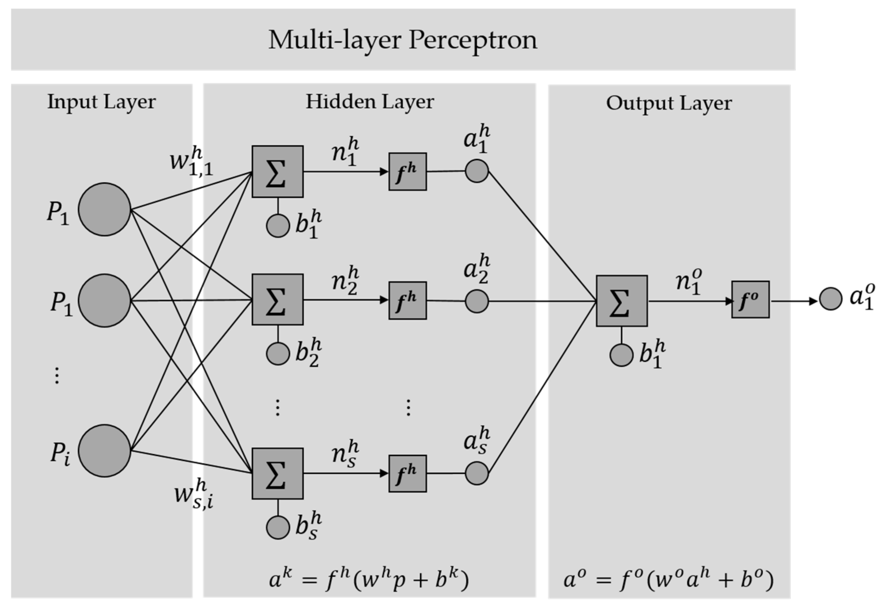
3.4. Prediction of Energy Consumption Using ANNs

According to Neto and Fiorelli [13], simulations and ANNs are both efficient for predicting energy consumption; however, each has its own benefits and drawbacks. In the case of simulation, it is possible to input the operating hours of home appliances by the user, however there are limitations in inputting other detailed information. In the case of ANNs, energy consumption can be predicted by quantifying nonlinear user information [13]. In this study, the ANN method was considered more appropriate to use because a large amount of user information could be integrated and considered.

ANNs are machine-learning algorithms proposed by McCulloch and Pitts [18]. When they were first proposed, implementing the learning models was complicated and there was lack of clear connection between the input and output data. Nevertheless, these issues were solved with the development of deep neural networks (DNNs) that combined the backpropagation algorithm with multi-layers with multiple nodes [19]. Owing to the proposal of new functions and algorithms, as well as improved computer hardware, it is now possible to implement DNN models with one or more hidden layers. DNN models can analyze vast amounts of elements that were previously overlooked for analysis, and it is now possible to implement prediction models to derive outputs through the weight of each node [20].

Figure 4 shows the basic structure of the ANN model described by Equation (2). R is the number of input variables and S is the number of hidden neurons. p represents each input variable, b each hidden layer, and w its weight. The weight of each calculated element is used as the input of the activation function. The output is derived through the sum of the weighted values [15]. The activation function utilized the most commonly used sigmoid function:

$$n_k^h = {\displaystyle \sum }_{j=1}^R{w}_{k_j}^h{p}_j+b_{b\prime }^{k}k = 1 to S.$$

(2)

When an ANN prediction model is created, hidden nodes and layers must be constructed, as shown in Figure 5. As there is no clear standard or methodology for this, it is necessary to find the optimal model with the lowest mean squared error (MSE) value after making as many attempts as possible. For successful learning, the minimum numbers of hidden nodes and layers must be larger than the number of input variables n, and the maximum number must not exceed 2n + 1 [21]. In this study, the ANN model was examined while the number of layers was increased from 1 to 9. In addition, for each number of layers, five cases were created with the minimum number of hidden nodes, the maximum number of hidden nodes, and three intermediate numbers. The model with the lowest MSE, i.e., the highest model performance, was examined.

To verify the performance of the model, three methods were used to construct the household member information input data, and the performance of the three cases were compared. As previously mentioned, influential elements were found through regression analysis. The performance of models using the influential elements as input data were compared to a model that used all the original variables as input data, as well as to a model that used the four household member data derived by a number of previous studies as input data.

The ANN prediction model for residential buildings in South Korea by Whaid and Kim [22] was implemented using 14,260-hour data of 20 apartment complexes in Seoul. Their model used the physical elements of the buildings that had optimal MSE values as input data. Research on a prediction model that integrates user information with the model based on such physical attributes is required.

Lee et al. [15] derived the energy consumption from the same buildings according to the behavioral patterns of the users, and implemented a DNN model for predicting energy consumption through six elements, i.e., gender, age, occupation, income, education level, and length of residency. Their prediction model exhibited 64% accuracy, indicating that the six elements had an impact on energy consumption. As the energy consumption was derived through simulation rather than records of actual energy consumption, the influence of the six elements must be verified through a comparison with the actual energy consumption. In addition, as the research was conducted based on annual energy consumption, it is difficult to determine detailed seasonal consumption and influential elements. It is also necessary to conduct research on different types of residential buildings, such as apartments and detached houses, as the research was based only on multi-family houses.

It is difficult to accurately measure data such as energy consumption in residential buildings owing to its spatiotemporal variability [23]. Data-based models are widely used because they can calculate results through repeated learning, even for cases with limited input variables. ANN techniques are actively used in various areas, as it is easy to identify relationships between different variables, and nonlinear correlations can be analyzed without analyzing the physical phenomena [24].

4. Results and Discussion

4.1. Derivation of Influential Elements

4.1.1. Analysis Process (Multi-Collinearity, Outliers, and Dependent and Independent Variables)

Prior to the analysis, among the 2520 households in 2016 and 2520 households in 2017, the following were removed as outliers: 92 households with unidentifiable data in each item, 2 households located on the 100th or higher floors, and 3 households where there were 4 or more household members aged 65 or older.

The data from all 16 regions comprised 12 physical building elements and 12 user information elements, as shown in

Table 1. Data construction, descriptive statistics, and variance inflation factor (VIF) analysis results.

Code	Variable	Category		Mean	Standard Deviation	N	Common Difference	VIF
city	City	11	Seoul *	−	−	−	−	−
		21	Pusan	00.0647	0.24609	4943	0.703	1.423
		22	Daegu	00.0475	0.21282	4943	0.778	1.285
		23	Incheon	00.0477	0.21325	4943	0.774	1.292
		24	Gwangju	00.0473	0.21239	4943	0.756	1.322
		25	Daejun	00.0471	0.21195	4943	0.791	1.264
		26	Ulsan	00.0324	0.17700	4943	0.818	1.222
		31	Kyunggi	0.1107	0.31374	4943	0.628	1.593
		32	Kangwon	00.0475	0.21282	4943	0.733	1.364
		33	Chungbuk	00.0453	0.20802	4943	0.744	1.345
		34	Chungnam	00.0637	0.24429	4943	0.667	1.500
		35	Jeonbuk	00.0473	0.21239	4943	0.714	1.402
		36	Jeonnam	00.0627	0.24247	4943	0.676	1.479
		37	Kyungbuk	00.0803	0.27181	4943	0.636	1.573
		38	Kyungnam	00.0807	0.27243	4943	0.626	1.598
		39	Jeju	00.0152	0.12225	4943	0.879	1.137
B_a1	Housing type	1	Detached	0.3862	0.48693	4943	0.400	2.500
		2	Apartment	0.4574	0.49823	4943	0.226	4.433
		3	Others *	−	−	−	−	−
B_a2	Number of floors	Numeric		8.22	7.805	4943	0.182	5.485
B_a3	Floor number	Numeric		4.34	4.943	4943	0.443	2.258
B_a4	Number of exterior walls	Numeric		4.33	1.278	4943	0.582	1.718
B_a5	Housing direction	1	East	0.1194	0.32425	4943	0.303	3.305
		2	West	00.0641	0.24501	4943	0.426	2.346
		3	South	0.4200	0.49361	4943	0.162	6.189
		4	North *	−	−	−	−	−
		5	Southeast	0.1993	0.39949	4943	0.224	4.473
		6	Southwest	0.1034	0.30448	4943	0.327	30.055
		7	Northeast	00.0299	0.17044	4943	0.610	1.640
		8	Northwest	00.0190	0.13660	4943	0.694	1.440
B_a6	Construction year	Numeric		3.82	1.298	4943	0.597	1.674
B_a7	Housing area	Numeric		3.17	0.867	4943	0.411	2.432
B_a8	Number of bedrooms (rooms)	Numeric		2.72	0.728	4943	0.488	20.050
B_a9	Number of exterior wall windows	Numeric		8.11	3.961	4943	0.737	1.357
B_a10	Main heating method	1	Individual	0.9092	0.28740	4943	0.785	1.274
		2	Central heating *	−	−	−	−	−
B_a11	Cooling method	1	Air conditioner	0.3045	0.46023	4943	0.180	5.558
		2	No air conditioner *	−	−	−	−	−
B_a12	Air conditioner set temperature	Numeric		3.13	20.049	4943	0.160	6.239
H_a1	Number of years occupied	Numeric		10.91	8.722	4943	0.154	6.513
H_a2	Housing ownership	1	Owned	0.7589	0.42782	4943	0.827	1.209
		2	Not owned *	−	−	−	−	−
H_a3	Number of household members	Numeric		2.97	1.242	4943	0.487	20.054
H_a4	Number of economically active household members	Numeric		1.45	0.767	4943	0.622	1.608
H_a5	Number of household members aged 65 or older	Numeric		0.47	0.743	4943	0.557	1.795
H_a6	Composition of household members	1	Children	00.0500	0.21790	4943	0.756	1.322
		2	No children *	−	−	−	−	−
H_a7	Gender of household head	1	Male	0.7499	0.43309	4943	0.742	1.348
		2	Female *	−	−	−	−	−
H_a8	Age of household head	Numeric		3.74	10.052	4943	0.486	20.056
H_a9	Education level of household head	1	High school graduate or below	0.5855	0.49269	4943	0.624	1.602
		2	University graduate or above *	−	−	−	−	−
H_a10	Occupation of household head	1	Regular employee	0.4965	0.50004	4943	0.360	2.775
		2	Temporary employee	00.0558	0.22963	4943	0.770	1.298
		3	Owner operator	0.2320	0.42218	4943	0.459	2.179
		4	Etc.	−	−	−	−	−
H_a11	Unusual features of household	1	Unusual features	00.0981	0.29750	4943	0.633	1.579
		2	General *	−	−	−	−	−
H_a12	Annual gross income	Numeric		3.67	1.862	4943	0.426	2.347

. Regional variables were applied to the analysis to use them as proxy variables that represent the geographic characteristics, social atmosphere, economic characteristics, and annual weather of each region. Among the user information data, the gender, age, education level, and occupation were analyzed using the information about the household head due to the nature of the data.

Nominal variables were determined by regression analysis through dummy coding. The reference variables of each dummy variable are as follows. The regional variables were based on Seoul, which exhibited the largest temperature changes in 2016 and 2017. In South Korea, as energy efficiency is lowest when a building faces north, coding was performed based on northward facing buildings. Other variables were analyzed based on items for which it was difficult to derive meaningful conclusions when analysis and interpretation were conducted. Variables that were relatively few in number were not applied.

Prior to the analysis, multi-collinearity verification was performed, which could potentially reveal independent variables with high correlations. If multi-collinearity occurs, correlations among independent variables may affect the analysis and lead to wrong results. Consequently, independent variables that have a significant impact on the dependent variable may appear meaningless, or the sign of the regression coefficient may change [25]. The multi-collinearity verification showed that there was no collinearity between the variables, because the variance inflation factor (VIF) value was less than 10 for all items.

Table 2. Model explanatory power and suitability analysis results.

	R	R2	Revised R2	Estimated Standard Error	Durbin–Watson	F	Significant Probability
Annual	0.346	0.120	0.111	5284.355	1.664	130.084	00.000
Spring	0.354	0.125	0.116	1643.510	1.674	140.031	00.000
Summer	0.377	0.142	0.134	7740.096	1.749	16.251	00.000
Fall	0.332	0.110	0.101	1263.190	1.661	120.081	00.000
Winter	0.351	0.123	0.114	25,570.053	1.674	13.778	00.000

shows that the regression analysis models for residential energy consumption in the annual period, spring, summer, fall, and winter were appropriate. The Durbin–Watson results were between 1.661 and 1.749; Durbin–Watson numbers close to 2 indicate that there is no autocorrelation. The explanatory power for residential energy consumption, which was the dependent variable of each independent variable, was found to be 12% (annual), 12.5% (spring), 14.2% (summer), 11% (fall), and 12.3% (winter). These values are low compared to previous studies on energy consumption in buildings. This appears to be because user attributes, which are sociological and humanistic elements, were included in the analysis in large quantities.

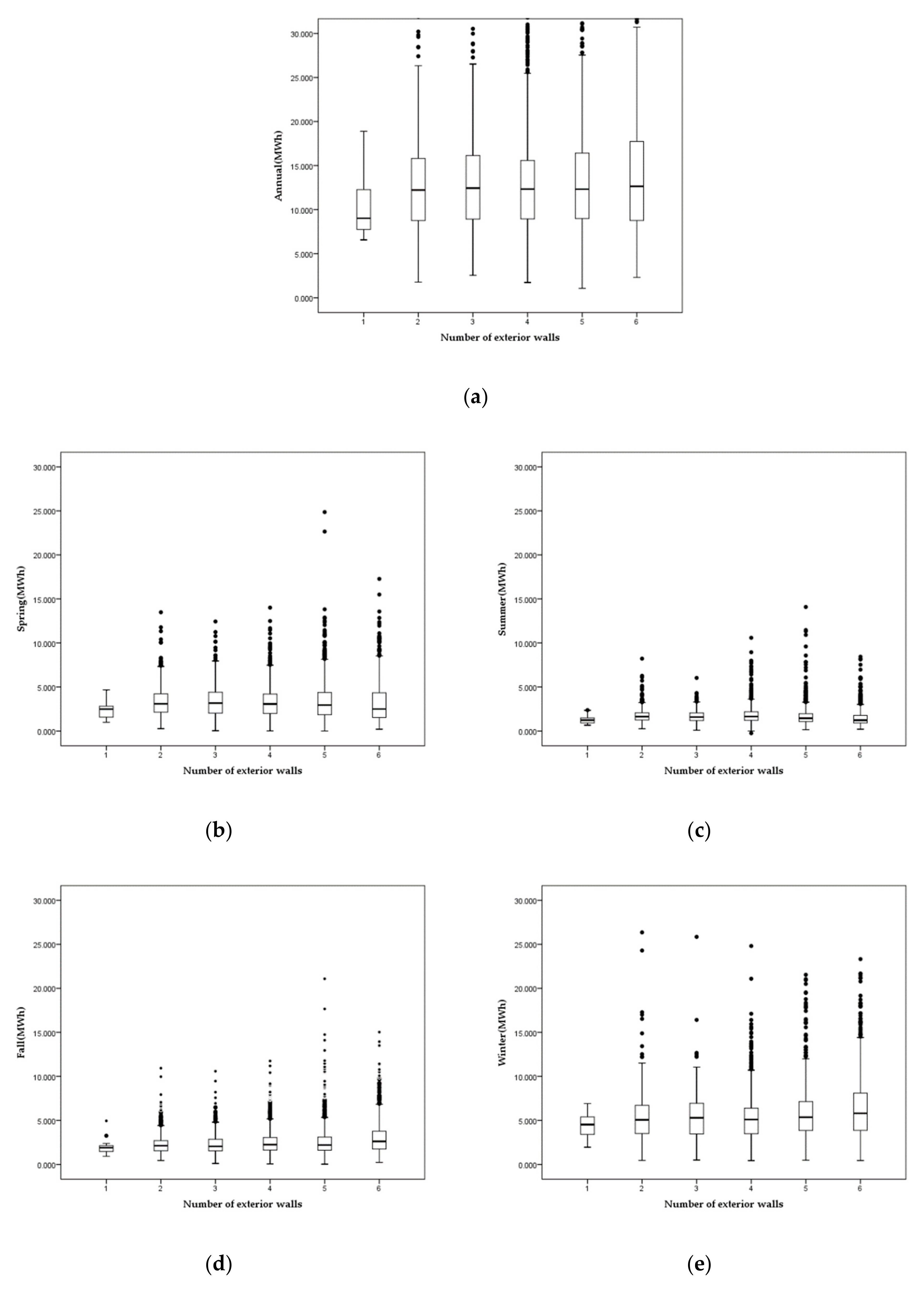
4.1.2. Elements Affecting Energy Consumption

Table 3. List of significant variables for seasonal residential building energy consumption.

Section	Code	Variable	Spring	Summer	Fall	Winter	Annual
Temp		Temperature	O		O
city		City	O	O	O	O	O
Building factors (12)	B_a1	Housing type		O	O	O	O
	B_a2	Number of floors				O
	B_a3	Floor number
	B_a4	Number of exterior walls	O	O	O	O	O
	B_a5	Housing direction	O	O	O	O	O
	B_a6	Construction year	O	O	O	O
	B_a7	Housing area	O	O	O	O	O
	B_a8	Number of bedrooms (rooms)		O
	B_a9	Number of exterior wall windows				O	O
	B_a10	Main heating method	O	O	O
	B_a11	Cooling method		O	O		O
	B_a12	Air conditioner set temperature			O	O
User features (12)	H_a1	Number of years occupied	O	O	O	O	O
	H_a2	Housing ownership
	H_a3	Number of household members	O	O	O	O	O
	H_a4	Number of economically active household members
	H_a5	Number of household members aged 65 or older		O
	H_a6	Composition of household members			O
	H_a7	Gender			O	O	O
	H_a8	Age of household head				O
	H_a9	Education level of household head				O
	H_a10	Occupation of household head	O	O	O	O	O
	H_a11	Unusual features of household		O		O
	H_a12	Annual gross income	O	O		O	O
Total			11	15	15	17	12

shows the physical elements and user attributes identified through the regression analysis as affecting residential energy consumption annually, as well as in the spring, summer, fall, and winter periods. The detailed results are given in the Appendix A

Table A1. Results of deriving elements that affect energy consumption in the annual period and spring.

	Annual					Spring
	Unstandardized Coefficient		Standardized Coefficient	t	p	Unstandardized Coefficient		Standardized Coefficient	t	p
	B	Standard Error				B	Standard Error
item	0.357	20.728	00.000	00.017	0.986	430.039	14.879	00.051	2.893	*** 00.004
cityD2	−1814.663	364.398	−00.080	−4.980	*** 00.000	−907.482	113.356	−0.128	−80.006	*** 00.000
cityD3	−1016.515	400.446	−00.039	−2.538	** 00.011	−391.367	126.351	−00.048	−30.097	*** 00.002
cityD4	814.586	400.820	00.031	20.032	** 00.042	308.361	127.427	00.038	2.420	** 00.016
cityD5	−11310.071	4070.010	−00.043	−2.779	*** 00.005	−741.729	126.291	−00.090	−5.873	*** 00.000
cityD6	−7080.094	398.812	−00.027	−1.776	* 00.076	−300.561	124.220	−00.036	−2.420	** 00.016
cityD7	433.798	469.603	00.014	0.924	0.356	−83.532	145.999	−00.008	−0.572	0.567
cityD8	291.769	302.461	00.016	0.965	0.335	−830.080	94.586	−00.015	−0.878	0.380
cityD9	2138.199	412.616	00.081	5.182	*** 00.000	219.506	129.448	00.027	1.696	* 0.090
cityD10	−1339.813	419.101	−00.050	−3.197	*** 00.001	−508.758	130.348	−00.061	−3.903	*** 00.000
cityD11	−40.925	376.899	−00.002	−0.109	0.914	−509.335	124.624	−00.071	−40.087	*** 00.000
cityD12	271.929	4190.089	00.010	0.649	0.516	−376.520	138.285	−00.046	−2.723	*** 00.006
cityD13	−9540.095	3770.056	−00.041	−2.530	00.011	−805.814	119.814	−0.112	−6.726	*** 00.000
cityD14	−260.189	346.897	−00.013	−0.750	0.453	−297.113	109.483	−00.046	−2.714	*** 00.007
cityD15	−1647.383	348.892	−00.080	−4.722	*** 00.000	−751.381	109.655	−0.117	−6.852	*** 00.000
cityD16	−30600.076	655.856	−00.067	−4.666	*** 00.000	−1345.139	202.957	−00.094	−6.628	*** 00.000
B_a1D1	732.460	244.133	00.064	30.000	*** 00.003	76.721	75.923	00.021	10.011	0.312
B_a1D2	−734.310	317.726	−00.065	−2.311	** 00.021	117.963	98.802	00.034	1.194	0.233
B_a2	33.173	22.561	00.046	1.470	0.142	2.494	70.016	00.011	.356	0.722
B_a3	−12.186	22.855	−00.011	−0.533	0.594	−3.610	7.105	−00.010	−0.508	0.611
B_a4	269.490	77.128	00.061	3.494	*** 00.000	81.979	240.000	00.060	3.416	*** 00.001
B_a5D1	−308.573	421.521	−00.018	−0.732	0.464	−156.118	1310.077	−00.029	−1.191	0.234
B_a5D2	173.711	4700.051	00.008	0.370	0.712	51.469	146.164	00.007	0.352	0.725
B_a5D3	−825.806	378.932	−00.073	−2.179	** 00.029	−243.738	117.820	−00.069	−20.069	** 0.039
B_a5D4	−577.103	3980.033	−00.041	−1.450	0.147	−1270.065	123.751	−00.029	−10.027	0.305
B_a5D5	−353.640	431.583	−00.019	−0.819	0.413	−87.611	134.185	−00.015	−0.653	0.514
B_a5D6	35.501	564.874	00.001	00.063	0.950	−42.340	175.641	−00.004	−0.241	0.810
B_a5D7	27400.077	660.559	00.067	4.148	*** 00.000	798.281	205.397	00.062	3.887	*** 00.000
B_a6	−64.802	74.977	−00.015	−0.864	0.387	53.711	23.309	00.040	2.304	** 00.021
B_a7	617.644	135.289	00.096	4.565	*** 00.000	1800.037	420.047	00.089	4.282	*** 00.000
B_a8	124.599	147.855	00.016	0.843	0.399	48.553	45.975	00.020	10.056	0.291
B_a9	50.639	22.108	00.036	2.291	** 00.022	10.929	6.854	00.025	1.595	0.111
H_a2	146.845	193.209	00.011	0.760	0.447	−0.575	600.077	00.000	−0.010	0.992
H_a1	81.183	21.999	0.126	3.690	*** 00.000	31.475	6.839	0.157	4.602	*** 00.000
H_a1′	−0.747	.495	−00.050	−1.509	0.131	−0.435	0.154	−00.094	−2.823	*** 00.005
B_a10D1	171.356	295.268	00.009	0.580	0.562	393.854	91.814	00.065	4.290	*** 00.000
B_a11D1	−6680.002	385.133	−00.055	−1.734	* 00.083	−127.971	110.536	−00.034	−1.158	0.247
B_a12	6.388	91.652	00.002	00.070	0.944	2.708	25.294	00.003	0.107	0.915
H_a3	462.611	86.738	0.103	5.333	*** 00.000	132.854	26.966	00.094	4.927	*** 00.000
H_a4	−44.999	124.266	−00.006	−0.362	0.717	−31.374	38.633	−00.014	−0.812	0.417
H_a5	−28.372	135.552	−00.004	−0.209	0.834	−39.405	42.151	−00.017	−0.935	0.350
H_a6D1	−29.574	396.759	−00.001	−00.075	0.941	70.830	123.367	00.009	0.574	0.566
H_a7D1	341.354	201.582	00.026	1.693	* 00.090	15.726	62.698	00.004	0.251	0.802
H_a8	1570.023	102.477	00.029	1.532	0.126	220.078	31.828	00.013	0.694	0.488
H−a9D1	−255.470	193.122	−00.022	−1.323	0.186	−78.738	600.050	−00.022	−1.311	0.190
H_a10D1	211.767	250.475	00.019	0.845	0.398	52.686	77.883	00.015	0.676	0.499
H_a10D2	4670.059	3730.087	00.019	1.252	0.211	126.967	1160.006	00.017	10.094	0.274
H_a10D3	762.147	262.911	00.057	2.899	*** 00.004	156.110	81.754	00.038	1.910	* 00.056
H_a11D1	−430.564	317.554	−00.023	−1.356	0.175	−143.325	98.641	−00.024	−1.453	0.146
H_a12	192.451	61.871	00.064	3.111	*** 00.002	53.379	19.237	00.057	2.775	*** 00.006

Note. * 90% Confidence interval (p-value < 0.10). ** 95% Confidence interval (p-value < 00.05). *** 99% Confidence interval (p-value < 00.01).

,

Table A2. Results of deriving elements that affect energy consumption in summer and fall.

	Summer					Fall
	Unstandardized Coefficient		Standardized Coefficient	t	p	Unstandardized Coefficient		Standardized Coefficient	t	p
	B	Standard Error				B	Standard Error
item	1.718	1.751	0.016	0.981	0.327	−6.695	30.084	−0.036	−2.171	** 0.030
cityD2	−30.664	53.397	−0.009	−0.574	0.566	−71.580	87.106	−0.013	−0.822	0.411
cityD3	−9.140	58.628	−0.002	−0.156	0.876	−204.944	960.022	−0.033	−2.134	** 0.033
cityD4	2360.065	58.826	0.061	40.013	*** 0.000	181.359	95.966	0.029	1.890	* 0.059
cityD5	340.312	59.359	0.087	5.733	*** 0.000	400.273	96.896	0.064	4.131	*** 0.000
cityD6	47.889	58.428	0.012	0.820	0.412	−75.236	95.503	−0.012	−0.788	0.431
cityD7	391.711	68.883	0.083	5.687	*** 0.000	255.787	112.213	0.034	2.279	** 0.023
cityD8	103.617	44.592	0.039	2.324	** 0.020	120.392	72.378	0.028	1.663	* 0.096
cityD9	185.195	60.793	0.047	30.046	*** 0.002	938.350	98.907	.150	9.487	*** 0.000
cityD10	−1100.012	61.396	−0.028	−1.792	* 0.073	−126.288	100.152	−0.020	−1.261	0.207
cityD11	−64.592	55.404	−0.019	−1.166	.244	388.833	900.043	0.071	4.318	*** 0.000
cityD12	1640.007	61.551	0.042	2.665	*** 0.008	492.574	100.279	0.079	4.912	*** 0.000
cityD13	162.858	55.292	0.047	2.945	*** 0.003	292.507	90.636	0.053	3.227	*** 0.001
cityD14	−46.584	50.822	−0.015	−0.917	0.359	102.193	82.815	0.021	1.234	0.217
cityD15	14.558	510.090	0.005	0.285	0.776	−108.530	83.428	−0.022	−1.301	0.193
cityD16	−201.902	95.623	−0.030	−2.111	** 0.035	−94.801	156.221	−0.009	−0.607	0.544
B_a1D1	−34.260	35.755	−0.020	−0.958	0.338	260.596	58.346	0.095	4.466	*** 0.000
B_a1D2	125.811	46.530	0.075	2.704	*** 0.007	−220.313	75.932	−0.082	−2.901	*** 0.004
B_a2	−0.182	3.304	−0.002	−0.055	0.956	8.567	5.392	0.050	1.589	0.112
B_a3	1.888	3.347	0.011	0.564	0.573	1.167	5.462	0.004	.214	0.831
B_a4	20.318	11.292	0.031	1.799	* 0.072	59.347	18.429	0.057	3.220	*** 0.001
B_a5D1	−1050.092	61.738	−0.041	−1.702	* 0.089	−28.303	100.742	−0.007	−0.281	0.779
B_a5D2	−89.253	68.842	−0.026	−1.296	0.195	29.479	112.338	0.005	0.262	0.793
B_a5D3	−144.406	55.502	−0.086	−2.602	*** 0.009	−184.830	90.565	−0.068	−20.041	** 0.041
B_a5D4	−101.954	58.298	−0.049	−1.749	* 0.080	−1480.091	95.132	−0.044	−1.557	0.120
B_a5D5	−20.276	63.213	−0.007	−0.321	0.748	−106.717	103.150	−0.024	−10.035	0.301
B_a5D6	−7.870	82.730	−0.002	−0.095	0.924	93.114	1350.002	0.012	0.690	0.490
B_a5D7	239.719	96.752	0.039	2.478	** 0.013	550.689	157.874	0.056	3.488	*** 0.000
B_a6	28.788	10.979	0.045	2.622	*** 0.009	−60.368	17.921	−0.059	−3.369	*** 0.001
B_a7	60.879	19.819	0.063	30.072	*** 0.002	117.791	32.336	0.077	3.643	*** 0.000
B_a8	37.742	21.655	0.033	1.743	* 0.081	20.892	35.337	0.011	0.591	0.554
B_a9	2.548	3.241	0.012	0.786	0.432	3.274	5.284	0.010	0.620	0.535
H_a2D1	−14.784	28.296	−0.008	−0.522	0.601	34.190	46.176	0.011	0.740	0.459
H_a1	120.076	3.222	0.127	3.748	*** 0.000	120.068	5.258	0.079	2.295	** 0.022
H_a1′	−0.223	0.073	−0.101	−30.070	*** 0.002	−0.076	0.118	−0.021	−0.640	0.522
B_a10D1	253.457	43.243	0.088	5.861	*** 0.000	−242.139	70.567	−0.052	−3.431	*** 0.001
B_a11D1	−207.917	56.601	−0.115	−3.673	*** 0.000	−308.712	92.132	−0.107	−3.351	*** 0.001
B_a12	−20.675	13.500	−0.051	−1.531	0.126	−40.965	21.942	−0.063	−1.867	** 0.062
H_a3	69.217	12.703	0.103	5.449	*** 0.000	76.511	20.732	0.071	3.690	*** 0.000
H_a4	7.816	18.199	0.007	0.429	0.668	31.957	29.700	0.018	10.076	0.282
H_a5	−33.428	19.852	−0.030	−1.684	* 0.092	−10.478	32.396	−0.006	−0.323	0.746
H_a6D1	−54.115	58.107	−0.014	−0.931	0.352	−54.274	94.823	−0.009	−0.572	0.567
H_a7D1	12.509	29.522	0.007	0.424	0.672	133.117	48.173	0.043	2.763	*** 0.006
H_a8	9.950	150.009	0.013	0.663	0.507	23.400	24.493	0.018	0.955	0.339
H_a9D1	18.369	28.285	0.011	0.649	0.516	−23.159	46.154	−0.009	−0.502	0.616
H_a10D1	8.149	36.683	0.005	0.222	0.824	88.442	59.861	0.033	1.477	0.140
H_a10D2	0.109	54.641	0.000	0.002	0.998	187.926	89.164	0.032	2.108	** 0.035
H_a10D3	70.701	38.506	0.036	1.836	* 0.066	166.152	62.833	0.053	2.644	*** 0.008
H_a11D1	−82.654	46.515	−0.030	−1.777	* 0.076	−109.995	75.904	−0.025	−1.449	0.147
H_a12	44.186	90.060	0.099	4.877	*** 0.000	180.026	14.788	0.025	1.219	0.223

Note. * 90% Confidence interval (p-value < 0.10). ** 95% Confidence interval (p-value < 00.05). *** 99% Confidence interval (p-value < 00.01).

and

Table A3. Results of deriving elements that affect energy consumption in winter.

	Winter
	Unstandardized Coefficient		Standardized Coefficient	t	p
	B	Standard Error
item	−0.723	16.868	−0.001	−0.043	0.966
cityD2	−7930.038	197.362	−0.072	−40.018	*** 0.000
cityD3	−363.774	199.398	−0.028	−1.824	* 0.068
cityD4	158.162	202.879	0.012	0.780	0.436
cityD5	−1142.696	223.802	−0.089	−5.106	*** 0.000
cityD6	−371.881	197.825	−0.029	−1.880	* 0.060
cityD7	−113.413	243.285	−0.007	−0.466	0.641
cityD8	179.269	1510.027	0.021	1.187	0.235
cityD9	738.232	214.639	0.058	3.439	*** 0.001
cityD10	−581.945	213.632	−0.045	−2.724	*** 0.006
cityD11	263.793	192.844	0.024	1.368	0.171
cityD12	118.786	218.915	0.009	0.543	0.587
cityD13	−546.911	195.663	−0.049	−2.795	*** 0.005
cityD14	−72.352	188.881	−0.007	−0.383	0.702
cityD15	−758.888	184.372	−0.076	−4.116	*** 0.000
cityD16	−1359.103	341.562	−0.061	−3.979	*** 0.000
B_a1D1	432.979	118.122	0.078	3.666	*** 0.000
B_a1D2	−761.329	153.708	−0.140	−4.953	*** 0.000
B_a2	22.486	10.915	0.065	20.060	** 0.039
B_a3	−11.662	110.057	−0.021	−10.055	0.292
B_a4	105.273	37.345	0.050	2.819	*** 0.005
B_a5D1	−24.133	203.936	−0.003	−0.118	0.906
B_a5D2	179.642	227.420	0.016	0.790	0.430
B_a5D3	−255.944	183.316	−0.046	−1.396	0.163
B_a5D4	−203.349	192.537	−0.030	−10.056	0.291
B_a5D5	−143.873	208.770	−0.016	−0.689	0.491
B_a5D6	−7.363	273.268	0.000	−0.027	0.979
B_a5D7	1141.306	319.547	0.057	3.572	*** 0.000
B_a6	−86.523	36.265	−0.041	−2.386	** 0.017
B_a7	256.882	65.425	0.082	3.926	*** 0.000
B_a8	18.179	71.536	0.005	0.254	0.799
B_a9	340.052	10.677	0.050	3.189	*** 0.001
H_a2D1	129.345	93.460	0.020	1.384	0.166
H_a1	25.484	10.642	0.082	2.395	** 0.017
H_a1’	−0.010	.240	−0.001	−0.042	0.966
B_a10D1	−232.919	142.860	−0.025	−1.630	0.103
B_a11D1	−13.605	176.178	−0.002	−0.077	0.938
B_a12	68.367	40.644	0.052	1.682	* 0.093
H_a3	185.219	41.961	0.085	4.414	*** 0.000
H_a4	−54.963	60.132	−0.016	−0.914	0.361
H_a5	560.098	65.579	0.015	0.855	0.392
H_a6D1	6.379	191.959	0.001	0.033	0.973
H_a7D1	175.735	97.560	0.028	1.801	* 0.072
H_a8	103.519	49.491	0.040	20.092	** 0.037
H_a9D1	−172.529	93.428	−0.031	−1.847	* 0.065
H_a10D1	64.481	121.169	0.012	0.532	0.595
H_a10D2	151.951	180.518	0.013	0.842	0.400
H_a10D3	371.304	127.200	0.058	2.919	*** 0.004
H_a11D1	−94.230	153.444	−0.010	−0.614	0.539
H_a12	77.452	29.931	0.053	2.588	** 0.010

Note. * 90% Confidence interval (p-value < 0.10). ** 95% Confidence interval (p-value < 00.05). *** 99% Confidence interval (p-value < 00.01).

the dummy-coded variables were analyzed through a comparison with the reference group. It was determined that energy consumption increased by the value of the non-standardized coefficient (B) when each of the continuous variables increased by 1.

In addition to the regional variables, it was found that among the physical elements of the building, the number of exterior walls, housing direction, and housing area were influential in all seasons. Among the user attributes, the number of years occupied, number of household members, and occupation of household head were found to be influential in all seasons. Figure 6, Figure 7, Figure 8, Figure 9, Figure 10 and Figure 11 show the annual and seasonal energy consumption distribution charts for these six elements.

Figure 6 shows the seasonal energy consumption distribution charts for the number of exterior walls. Exterior walls refer to walls that directly face the outside air. The number of exterior walls is a continuous variable, from 0 (for the basement) to 6. As shown in the figure, energy consumption showed a tendency to increase as the number of exterior walls increased, because exterior walls are vulnerable to insulation and release heat to the surroundings [19].

The housing direction is the direction that the front of the building faces. In South Korea, it is usually determined based on the position of the living room [26]. This is because Korean users spend a considerable amount of time in the living room. In South Korea, north-facing walls have the lowest daily average solar radiation, resulting in low energy efficiency. Hence, houses are usually designed to avoid the north. The reference variable therefore considered buildings in a north facing direction. The analysis results in Figure 7 show that energy consumption was highest in the northwest direction and lowest in the south direction. This indicates that the northwest direction is more vulnerable to residential energy consumption than the north direction, which is the reference variable, in South Korea.

In South Korea, the “pyeong” unit is usually used in calculating the area of a building. 1 pyeong corresponds to 3.3 m². Five groups were prepared with intervals of 33 m² (10 pyeong) to analyze the effect of housing area. As the area relates to the volume of the building and therefore the volume of internal air, buildings with larger areas are more vulnerable to energy consumption [27]. Figure 8 shows that energy consumption generally increased as the building area increased.

Time-related variables, such as construction year and number of years occupied, may form a curved distribution. In such cases, general regression analysis for analyzing linear samples may not produce significant results. Nevertheless, regression analysis can be used if the data is converted to a linear distribution by squaring the value of each point. In the case of the construction year, significant results were not obtained. However, for the number of years occupied, a point of inflection appeared between 4 and 6 years, as shown in Figure 9, indicating that the variable had a curve-type distribution. This suggests that energy consumption increases with an increase in number of years occupied up to 4–6 years, but decreases afterward.

Energy consumption increases as the number of household members increases, because there are more users that directly consume energy. As shown in Figure 10, energy consumption showed a tendency to increase as the number of household members increased in the annual period and all seasons. Moreover, the number of household members appear to be more influential in winter and spring, when energy related to heating and hot water are consumed more frequently, than in summer, when cooling-related energy is consumed.

For ordinary households in South Korea, the household head is responsible for all household members. The occupation of the household head was applied as occupational data in this study; the occupation was classified as regular employees, temporary employees, business owners, and others. The analysis results showed that business owners had an influence on energy consumption in most periods as shown in Figure 11. This is because many business owners in South Korea use homes for business and residence, and thus their residence time is longer than that of other occupations.

In addition to the six common influential elements, the elements that had an influence in each season are as follows. The temperature was found to be more influential in spring and fall when considered in a comprehensive manner. Detached houses were found to be more vulnerable to higher energy consumption in all periods other than spring. Energy consumption showed a tendency to increase for all seasons as buildings became older, but the influence of building age was lower than that of other elements on an annual basis. The number of exterior walls was only influential in winter and annual periods, while the main heating method was influential in the spring, summer, and fall. The cooling method was influential in summer, fall, and the annual period, and energy consumption was affected by the air conditioner set temperature in fall and winter. Occupant gender had an influence on energy consumption in fall, winter, and the annual period, and the unusual features of household were influential in summer and winter. The annual gross income was influential in all periods except fall. Several elements exhibited an influence in specific seasons. In summer, energy consumption varied depending on the number of bedrooms and the number of household members aged 65 or older. In fall, it varied depending on the composition of household members. In winter, the number of floors, the age of household head, and the education level of the household head were found to be influential.

4.2. Energy Consumption Prediction Model

4.2.1. Input/Output Data

The ANN model was constructed for five periods (annual, spring, summer, fall, and winter). Elements that were found to be influential in each season were selected as input variables for the analysis. In the case of nominal variables, the ANN model was constructed by including the reference group as input variables after performing dummy coding. When the input variables of each model were examined based on the significant elements, it was found that the number of input variables were as follows: 42 for the annual model, 38 for the spring model, 46 for the summer model, 47 for the fall model, and 48 for the winter model.

As shown in

Table 4. Information on the use of data.

No. of Samples	Training	Validation	Testing
4943	70%	15%	15%
	3461	741	741

, 4943 data were used for the analysis, excluding outliers. Among them, 3461 data were used for training, 741 for validation, and 741 for testing.

4.2.2. Hidden Layer and Node

Table 5. Performances of seasonal energy consumption prediction models according to the hidden layers.

Period	Min	Max	Layer	Neuron	R Value of Training	R Value of Validation	R Value of Test	MSE	Terminated Epoch
Annual	42	85	1	70	0.257	0.303	0.278	${10}^7$ × 2.5250	12th
			2	35	0.351	0.279	0.306	${10}^7$ × 2.7545	5th
			3	21	0.419	0.299	0.312	${10}^7$ × 3.4674	5th
			4	11	0.361	0.288	0.262	${10}^7$ × 2.6649	4th
			5	13	0.427	0.270	0.272	${10}^7$ × 2.8077	7th
			6	14	0.535	0.348	0.256	${10}^7$ × 3.1436	12th
Spring	38	77	1	47	0.363	0.296	0.235	${10}^6$ × 2.6339	14th
			2	24	0.391	0.284	0.279	${10}^6$ × 2.5981	5th
			5	8	0.477	0.312	0.246	${10}^6$ × 2.7300	7th
			6	12	0.457	0.256	0.331	${10}^6$ × 2.7304	4th
			7	6	0.376	0.283	0.324	${10}^6$ × 2.7068	8th
			8	7	0.404	0.278	0.317	${10}^6$ × 2.6193	9th
Summer	46	93	1	58	0.322	0.315	0.283	${10}^5$ × 5.3157	12th
			2	23	0.543	0.264	0.243	${10}^5$ × 7.9380	5th
			3	16	0.382	0.318	0.270	${10}^5$ × 5.1060	7th
			4	17	0.382	0.247	0.213	${10}^5$ × 6.1292	2nd
			5	10	0.450	0.389	0.353	${10}^5$ × 5.4341	8th
			6	8	0.442	0.342	0.372	${10}^5$ × 5.9818	6th
Fall	47	95	1	47	0.336	0.278	0.217	${10}^6$ × 1.4318	27th
			2	30	0.152	0.158	0.131	${10}^6$ × 1.6054	19th
			3	16	0.399	0.273	0.201	${10}^6$ × 1.6571	3rd
			4	17	0.288	0.208	0.167	${10}^6$ × 1.8019	3rd
			5	10	0.423	0.248	0.293	${10}^6$ × 1.6133	4th
			6	15	0.565	0.244	0.316	${10}^6$ × 1.8063	7th
Winter	48	97	1	84	0.336	0.287	0.261	${10}^6$ × 6.1731	15th
			2	24	0.287	0.234	0.212	${10}^6$ × 5.7602	8th
			3	24	0.732	0.359	0.336	${10}^6$ × 5.9531	2nd
			4	18	0.425	0.293	0.256	${10}^6$ × 5.9060	11th
			6	16	0.402	0.182	0.241	${10}^6$ × 7.2293	3rd
			7	13	0.485	0.252	0.293	${10}^6$ × 6.3134	4th

shows six cases with the highest model performances for each seasonal prediction model according to the number of layers. Gradient vanishing, in which prediction models cannot be used when the number of layers exceeds the number presented in the table, occurred.

4.2.3. ANN Simulation Result

Figure 12 shows the R-values of the training, validation, and test data of the highest performing annual energy consumption prediction model. The R-value was found to be 0.25745 for the training data, 0.30359 for the validation data, and 0.27886 for the test data. The MSE value was ${10}^7$ × 2.5250. This model had one layer and 70 nodes. It was found that the neural network (NN) model exhibited the highest performance.

Figure 13 shows the R-values of the training, validation, and test data of the highest performing spring energy consumption prediction model. The R-value was found to be 0.39154 for the training data, 0.28441 for the validation data, and 0.27913 for the test data. The MSE value was ${10}^6$ × 2.5981, and the model had two layers and 24 nodes. It was found that the DNN model with two layers exhibited the highest performance.

Figure 14 shows the R-values of the training, validation, and test data of the highest performing summer energy consumption prediction model. The R-value was 0.38204 for the training data, 0.31832 for the validation data, and 0.27092 for the test data. The MSE value was ${10}^5$ × 5.1060, and the model had three layers and 16 nodes. It was found that the DNN model with three layers exhibited the highest performance.

Figure 15 shows the R-values of the training, validation, and test data of the highest performing fall energy consumption prediction model. The R-value was 0.33652 for the training data, 0.2783 for the validation data, and 0.21787 for the test data. The MSE value was ${10}^6$ × 1.4318, and the model had one layer and 47 nodes. It was found that the NN model with one layer exhibited the highest performance.

Figure 16 shows the R-values of the training, validation, and test data of the highest performing winter energy consumption prediction model. The R-value was 0.28741 for the training data, 0.23453 for the validation data, and 0.21289 for the test data. The MSE value was ${10}^6$ × 5.7602. This model had two layers and 24 nodes. It was found that the DNN model with two layers exhibited the highest performance.

For the annual and fall periods, the performances of the NN models with one layer were found to be excellent. However, the DNN models with two or more layers did not have significantly different MSE values. This indicates that if a sufficient amount of data from the Household Energy Standing Survey were used, the model performance would be improved and the application of DNN models will be possible.

Table 6. Performances of seasonal energy consumption prediction models according to the input data type.

Period	Input Type	Layer	Neuron	R Value of Training	R Value of Validation	R Value of Test	MSE	Terminated Epoch
Annual	A	1	70	0.257	0.303	0.278	${10}^7$ × 2.5250	12th
	B	1	70	0.327	0.238	0.262	${10}^7$ × 3.160	17th
	C	1	70	0.320	0.215	0.270	${10}^7$ × 4024	24th
Spring	A	2	24	0.391	0.284	0.279	${10}^6$ × 2.5981	5th
	B	2	24	−	−	−	−	−
	C	2	24	0.724	0.363	0.297	${10}^6$ × 3.2416	9th
Summer	A	3	16	0.382	0.318	0.270	${10}^5$ x 5.1060	7th
	B	3	16	−	−	−	−	−
	C	3	16	0.629	0.279	0.339	${10}^5$ × 7.6997	6th
Fall	A	1	47	0.336	0.278	0.217	${10}^6$ × 1.4318	27th
	B	1	47	0.260	0.168	0.297	${10}^6$ × 1.5061	15th
	C	1	47	0.374	0.326	0.245	${10}^6$ × 1.6476	15th
Winter	A	2	24	0.287	0.234	0.212	${10}^6$ × 5.7602	8th
	B	2	24	0.588	0.375	0.220	${10}^6$ × 6.4005	4th
	C	2	24	0.477	0.287	0.318	${10}^6$ × 6.3853	6th

compares models with three input data types. The type A prediction models were constructed by conducting regression analysis on the household information elements of the original data, with the influential elements from each season set as input data. The type B prediction models were constructed using all 12 sets of household data as input data for all seasons. The type C prediction models were constructed by applying elements commonly derived as influential elements in previous studies as input data, i.e., the income, number of household members, occupation, composition of household members, etc.

To compare standards for household information, influential elements for each season were applied to models A, B, and C in the same manner as the physical elements of buildings. The same numbers of layers and neurons were also applied to types A, B, and C to control the influence of other factors except the input data of the model. The analysis results showed that type A, which used significant household information as input data in all seasons through regression analysis, exhibited the highest model accuracy. For type B, which used the original data, gradient vanishing occurred in the spring and summer models. Type C had higher prediction accuracy than type A, except in the annual period; however, there was a significant difference in prediction accuracy between the training and test models, resulting in an overfitting problem.

Based on the comparison and analysis results of each model, it was found that identifying the most significant variables through regression analysis could improve model performance, especially when variables that are difficult to quantify, such as household information, are included as input data.

5. Conclusions

An increasing number of studies have been conducted on the energy consumption of residential buildings. This study is different from previous studies in three aspects. First, this study was conducted based on the actual energy consumption of residential buildings in South Korea. Furthermore, the elements were derived by integrating the physical information of buildings with user information and reflecting mutual influence. Finally, energy consumption prediction models were implemented by dividing energy consumption into four seasons and deriving influential elements for each season.

This study found that user information has as much influence on energy consumption as the physical elements of buildings. In each season, the influence of the physical characteristics of buildings and household characteristics as well as the importance of each element was identified. The three representative elements that exhibited the highest influence in each season are as follows.

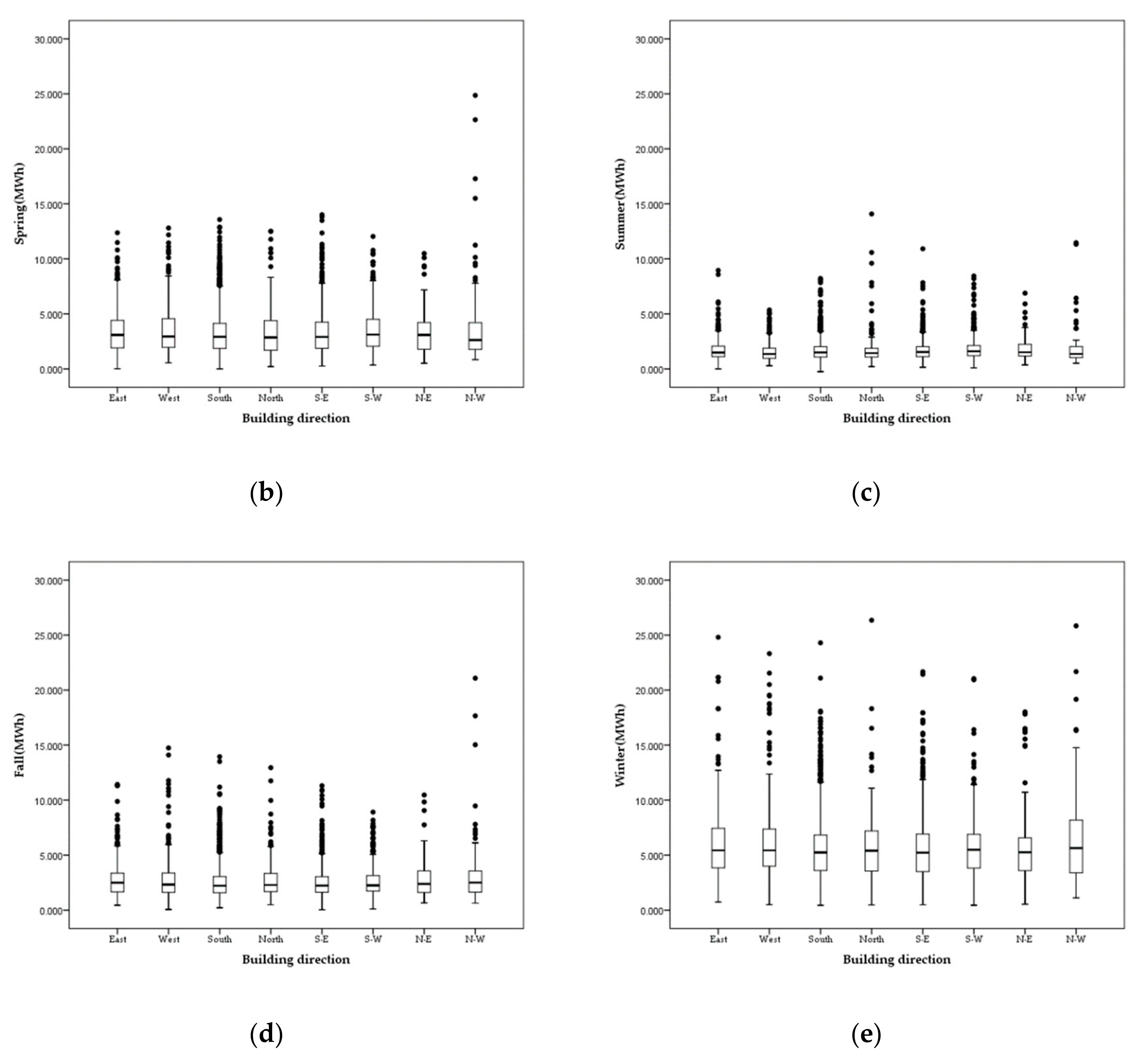
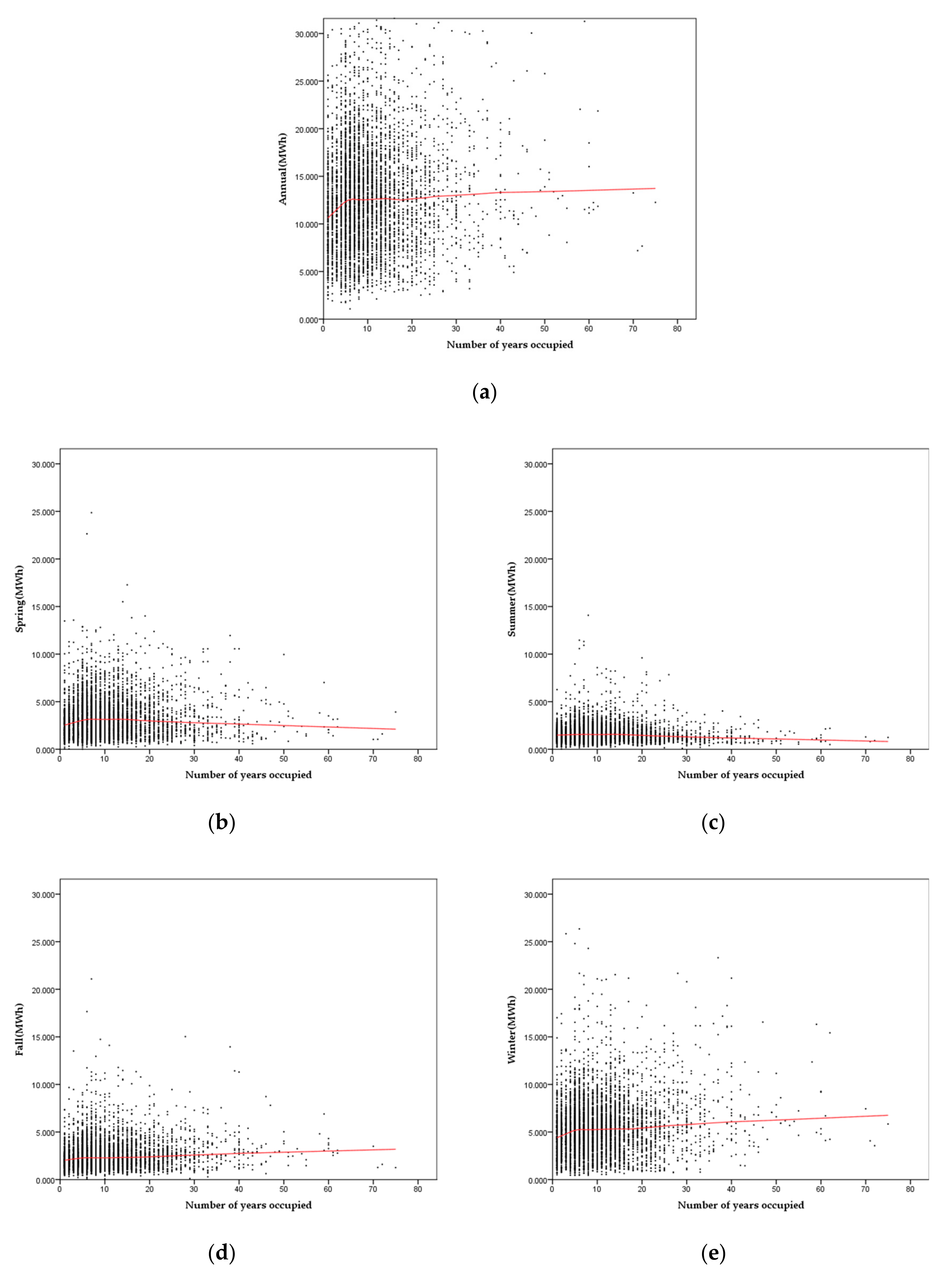
• In spring, the building direction was found to be the most influential element, followed by the occupation and cooling method. Buildings facing northwest—the direction with the lowest annual average solar radiation—exhibited the highest energy consumption. Buildings inhabited by to business owners, who typically have longer residence times than other occupations, also consumed more energy. Households that used air conditioners for cooling consumed more energy.
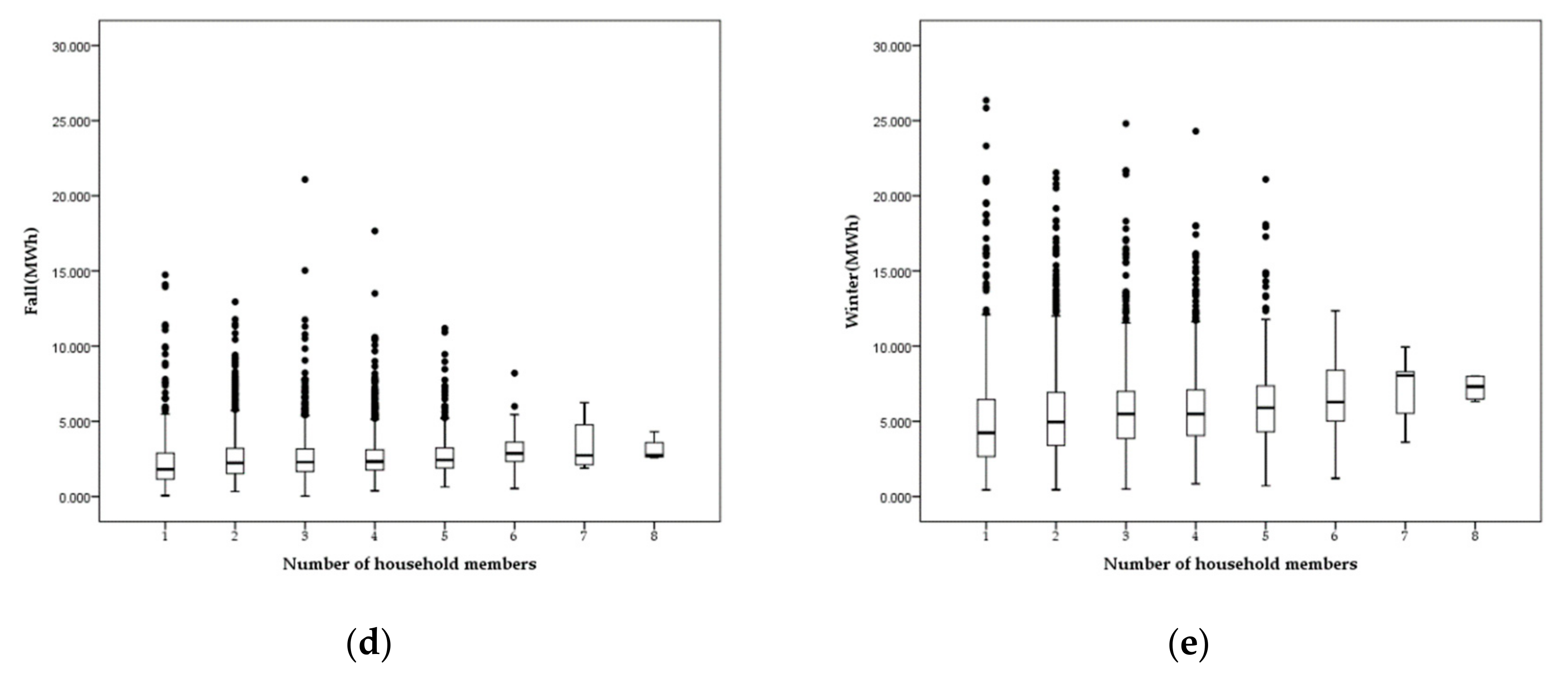
• In summer, the heating method was the most influential, followed by the cooling method and housing area. For residential buildings in South Korea, individual heating and central heating are the two representative heating methods. Households with individual heating were found to consume more energy. Heating energy was mostly concentrated on the use of hot water in summer, indicating that individual heating was more vulnerable to the use of energy related to hot water. As in spring, households that used air conditioners consumed more energy, as did households with larger areas.
• In fall, the housing area was the most influential factor, followed by the housing type and occupation. Households with larger areas consumed more energy, as did detached houses that managed energy individually. As in spring, buildings inhabited by to business owners exhibited the highest energy consumption.
• In winter, the building direction was the most influential, followed by the housing area and occupation. As in spring, the northwest direction with the lowest solar radiation exhibited the highest energy consumption. As the housing area increased, energy consumption increased. As for the occupation, to business owners with the longest residence time exhibited the highest energy consumption, as in spring and fall.

As seen above, different elements affected energy consumption in each season. The various elements had different influences depending on the season. This must be reflected when preparing systematic energy saving and management measures in the future. Providing data on seasonal energy usage will be possible when people with households displaying specific features will live in the target residential area. If enough information is obtained via matching these users with residential buildings, more sophisticated policies can be implemented, and greater awareness of energy use can be aroused individually. Such measures could be further developed by adding impact-reflecting factors and expanding the scope of the analysis in order to continuously reduce energy.

The suitability of the energy consumption prediction models implemented in this study was compared through a comparison of three types. For type A, a prediction model was constructed using the influential variables of each season derived through regression analysis as input data. For type B, a prediction model was constructed using the four representative user information elements derived in previous studies, i.e., the income, occupation, composition of household members, and number of household members. For type C, a prediction model was constructed using all the household information included in the original data. When the models were compared, it was found that type A exhibited the highest suitability. This indicates that prediction models with a higher performance can be implemented by verifying the influence of individual elements through regression analysis. It can then be applied to future prediction models that measure how atypical data affects energy consumption, such as the household member information. Predictive models of type B can identify influential factors and provide information that can be utilized when drafting a plan for continuous energy reduction from simple usage forecasting. Based on the influence of these individual factors, it is possible to formulate countermeasures in related fields when developing sustainable energy saving measure.

Currently, in South Korea, when evaluating the energy impact of users and buildings, the post-occupancy evaluation (POE) method is used to evaluate the energy impact of users and buildings. If the energy impact of the building and the user can be predicted using the model such as the one proposed in this study, a novel form of energy impact assessment can be conducted. Such assessments can reduce the unreasonable energy consumption of post-occupancy assessments and, furthermore, provide a way to create customized energy-saving residential spaces provided by both, the state or by individuals to create their own living environments.

In the model of this study, although the prediction rate increased by using only influential factors through regression analysis, the performance of the predictive model was limited because only two years’ worth of data were used. However, the dataset used in this study, the Household Energy Standing Survey, is conducted annually; hence, the current limitations owing to this lack of data will be eventually overcome.

The seasonal influential elements derived in this study are expected to be utilized as basic elements that can be used for further research on more accurate energy prediction if they are integrated with the information on detailed climate and building information, such as microclimate information, and information on the ownership and usage of home appliances. Such attempts will be useful as basic research to derive and predict common elements that have an influence on energy consumption on a national level, beyond residential energy research in the scope of single buildings and survey-based investigations in small areas.

References

1. U.S. Energy Information Administration. Annual Energy Outlook 2019; Government Printing Office: Washington, DC, USA, 2019. [Google Scholar]
2. Korea Energy Economics Institute. 2018 Energy Info. Korea; Yong-Sung Cho: Seoul, Korea, 2018. [Google Scholar]
3. Santamouris, M. Cooling the buildings–past, present and future. Energy Build. 2016, 128, 617–638. [Google Scholar] [CrossRef]
4. Kim, M.-K. An Estimation Model of Residential Building Electricity Consumption in Seoul. Seoul Stud. 2013, 14, 179–192. [Google Scholar]
5. Kim, Y.-L.; Hong, W.-H.; Seo, Y.-K.; Jeon, G.-Y. A Study on the Electricity Consumption Propensity by Household Members in Apartment Houses. J. Korean Hous. Assoc. 2011, 22, 43–50. [Google Scholar] [CrossRef] [Green Version]
6. Eum, M.-R.; Hong, W.-H.; Lee, J.-A. Deriving Factors Affecting Energy Usage for Improving Apartment Energy Consumption Evaluation. J. Archit. Inst. Korea Struct. Constr. 2018, 34, 27–34. [Google Scholar]
7. Lee, K.-H.; Chae, C.-U. Estimation Model of the Energy Consumption under the Building Exterior Conditions in the Apartment Housing—Focused on the Maintenance Stage. J. Archit. Inst. Korea Plan. Des. 2008, 24, 85–92. [Google Scholar]
8. Van den Brom, P.; Meijer, A.; Visscher, H. Performance gaps in energy consumption: Household groups and building characteristics. Build. Res. Inf. 2018, 46, 54–70. [Google Scholar] [CrossRef] [Green Version]
9. Schipper, L.; Bartlett, S.; Hawk, D.; Vine, E. Linking life-styles and energy use: A matter of time? Annu. Rev. Energy 1989, 14, 273–320. [Google Scholar] [CrossRef]
10. Noh, S.C.; Lee, H.Y. An analysis of the factors affecting the energy consumption of the household in Korea. J. Korea Plan. Assoc. 2013, 48, 295–312. [Google Scholar]
11. Jung, J.; Yi, C.; Lee, S. An integrative analysis of the factors affecting the household energy consumption in Seoul. J. Korea Plan. Assoc. 2015, 50, 75. [Google Scholar] [CrossRef]
12. Kim, K.; An, Y.; Seungil, L. Analysis of influencing factors of building and urban planning on building energy consumption considering income gap-focused on electricity consumption on August in Seoul. J. Korea Plan. Assoc. 2017, 52, 253–267. [Google Scholar]
13. Neto, A.H.; Fiorelli, F.A.S. Comparison between detailed model simulation and artificial neural network for forecasting building energy consumption. Energy Build. 2008, 40, 2169–2176. [Google Scholar] [CrossRef]
14. Seo, H.-C.; Hong, W.-H.; Nam, G.-M. Characteristics of Electric-Power Use in Residential Building by Family Composition and Their Income Level. J. Korean Hous. Assoc. 2012, 23, 31–38. [Google Scholar] [CrossRef]
15. Lee, S.; Jung, S.; Lee, J. Prediction model based on an artificial neural network for user-based building energy consumption in South Korea. Energies 2019, 12, 608. [Google Scholar] [CrossRef] [Green Version]
16. Domestic Climate Data. Available online: http://www.weather.go.kr/weather/climate/average_south.jsp (accessed on 5 October 2019).
17. Benítez, J.M.; Castro, J.L.; Requena, I. Are artificial neural networks black boxes? IEEE Trans. Neural Netw. 1997, 8, 1156–1164. [Google Scholar] [CrossRef]
18. McCulloch, W.S.; Pitts, W. A logical calculus of the ideas immanent in nervous activity. Bull. Math. Biol. 1990, 52, 99–115. [Google Scholar] [CrossRef]
19. Rumelhart, D.E.; Hinton, G.E.; Williams, R.J. Learning representations by back-propagating errors. Nature 1986, 323, 533–536. [Google Scholar] [CrossRef]
20. Salakhutdinov, R.; Mnih, A.; Hinton, G. Restricted Boltzmann machines for collaborative filtering. In Proceedings of the 24th International Conference on Machine Learning, Corvalis, OR, USA, 20–24 June 2007; ACM: New York, NY, USA, 2007; pp. 791–798. [Google Scholar]
21. Huang, W.; Foo, S. Neural network modeling of salinity variation in Apalachicola River. Water Res. 2002, 36, 356–362. [Google Scholar] [CrossRef]
22. Wahid, F.; Kim, D.H. Short-term energy consumption prediction in korean residential buildings using optimized multi-layer perceptron. Kuwait J. Sci. 2017, 44, 67–77. [Google Scholar]
23. Akhtar, M.; Corzo, G.; Van Andel, S.; Jonoski, A.; Sciences, E.S. River flow forecasting with artificial neural networks using satellite observed precipitation pre-processed with flow length and travel time information: Case study of the Ganges river basin. Hydrology 2009, 13, 1607–1618. [Google Scholar]
24. Park, J.-A.; Kim, G.-S. Estimation of spatial distribution of soil moisture at Yongdam dam watershed using artificial neural networks. J. Korean Geogr. Soc. 2011, 46, 319–330. [Google Scholar]
25. Pan, D.; Chan, M.; Deng, S.; Lin, Z.; Energy, J.A. The effects of external wall insulation thickness on annual cooling and heating energy uses under different climates. Appl. Energy 2012, 97, 313–318. [Google Scholar] [CrossRef]
26. Suh, D.; Chang, S. A heuristic rule-based passive design decision model for reducing heating energy consumption of Korean apartment buildings. Energies 2014, 7, 6897–6929. [Google Scholar] [CrossRef] [Green Version]
27. Yeo, M.-S.; Yang, I.-H.; Kim, K.-W. Historical changes and recent energy saving potential of residential heating in Korea. Energy Build. 2003, 35, 715–727. [Google Scholar] [CrossRef]
Figure 1. Research process.
Sustainability 12 00109 g001
Figure 2. Monthly average temperature distribution in 16 regions of South Korea; (a) 2016; (b) 2017.
Sustainability 12 00109 g002
Figure 3. Household energy consumption distribution by season; (a) spring; (b) summer; (c) fall; (d) winter.
Sustainability 12 00109 g003aSustainability 12 00109 g003b
Figure 4. Artificial neural network (ANN) model structure.
Sustainability 12 00109 g004
Figure 5. Structure of a seasonal energy consumption prediction model.
Sustainability 12 00109 g005
Figure 6. Seasonal energy consumption according to the number of exterior walls: (a) annual; (b) spring; (c) summer; (d) fall; (e) winter.
Sustainability 12 00109 g006
Figure 7. Seasonal energy consumption according to building direction: (a) annual; (b) spring; (c) summer; (d) fall; (e) winter.
Sustainability 12 00109 g007aSustainability 12 00109 g007b
Figure 8. Seasonal energy consumption according to building area: (a) annual; (b) spring; (c) summer; (d) fall; (e) winter.
Sustainability 12 00109 g008
Figure 9. Seasonal energy consumption according to the number of years occupied: (a) annual; (b) spring; (c) summer; (d) fall; (e) winter.
Sustainability 12 00109 g009
Figure 10. Seasonal energy consumption according to the number of household members: (a) annual; (b) spring; (c) summer; (d) fall; (e) winter.
Sustainability 12 00109 g010aSustainability 12 00109 g010b
Figure 11. Seasonal energy consumption according to the occupation of household head: (a) annual; (b) spring; (c) summer; (d) fall; (e) winter.
Sustainability 12 00109 g011aSustainability 12 00109 g011b
Figure 12. Annual energy consumption prediction model (layer: 1, node: 70); (a) Training data regression result; (b) Validation data regression result; (c) Test data regression result.
Sustainability 12 00109 g012
Figure 13. Spring energy consumption prediction model (layer: 2, node: 24); (a) Training data regression result; (b) Validation data regression result; (c) Test data regression result.
Sustainability 12 00109 g013
Figure 14. Summer energy consumption prediction model (layer: 3, node: 16); (a) Training data regression result; (b) Validation data regression result; (c) Test data regression result.
Sustainability 12 00109 g014
Figure 15. Fall energy consumption prediction model (layer: 1, node: 47); (a) Training data regression result; (b) Validation data regression result; (c) Test data regression result.
Sustainability 12 00109 g015
Figure 16. Winter energy consumption prediction model (layer: 2, node: 24); (a) Training data regression result; (b) Validation data regression result; (c) Test data regression result.
Sustainability 12 00109 g016