A Compact Pigeon-Inspired Optimization for Maximum Short-Term Generation Mode in Cascade Hydroelectric Power Station

Abstract

Pigeon-inspired optimization (PIO) is a new type of intelligent algorithm. It is proposed that the algorithm simulates the movement of pigeons going home. In this paper, a new pigeon herding algorithm called compact pigeon-inspired optimization (CPIO) is proposed. The challenging task for multiple algorithms is not only combining operations, but also constraining existing devices. The proposed algorithm aims to solve complex scientific and industrial problems with many data packets, including the use of classical optimization problems and the ability to find optimal solutions in many solution spaces with limited hardware resources. A real-valued prototype vector performs probability and statistical calculations, and then generates optimal candidate solutions for CPIO optimization algorithms. The CPIO algorithm was used to evaluate a variety of continuous multi-model functions and the largest model of hydropower short-term generation. The experimental results show that the proposed algorithm is a more effective way to produce competitive results in the case of limited memory devices.

1. Introduction

The metaheuristic algorithm [1] has emerged as a very promising tool to solve complex optimization problems. Original pigeon-inspired optimization (OPIO) is a new type of metaheuristic search algorithm [2]. The algorithm simulates the behavior of pigeons going home. Preliminary studies indicate that it is a very promising optimization algorithm and can outperform excellent existing algorithms [3]. OPIO exploits a population of pigeons as candidate solutions by setting boundaries and optimizing the problem by moving the candidate solutions to approach the best solutions based on a given measure of quality. The general steps of the algorithm are described below.

OPIO can solve continuous solution space problems. In addition, many versions of OPIO in the literature are proposed to solve the problem of continuous and discrete solution spaces in recent years. An improved Gaussian pigeon inspired optimization algorithm preserves the diversity of early evolution to avoid premature convergence. The entire algorithm shows excellent performance in global optimization and is effective for solving multimodal and non-convex problems with higher dimensions. Multi-objective pigeon-inspired optimization (MPIO) is used for multi-objective optimization in designing the parameters of brushless direct current motors  [4]. The multimodal multi-objective pigeon-inspired optimization algorithm (MMPIO) was proposed to figure out the multimodal multi-objective optimization problems [5,6].

With the continuous development of metaheuristic algorithms, intelligent group optimization has become an emerging technology to solve many engineering problems. Metaheuristic algorithms perform well on wireless sensor networks [7,8]. Since 2000, many scholars have designed many ant colony optimization algorithms, particle swarm optimization algorithms (PSO) [9], gray wolf optimization algorithms (GWO) [10,11], bat inspired algorithms (BA) [12,13], flower pollination algorithms (FPA) [14,15], cat swarm optimization (CSO) [16,17], differential evolution algorithm (DE) [18,19], quasi-affine transformation evolution algorithms (QUATRE) [20,21], genetic algorithms (GA) [22,23], etc. Based on the simulation of the above-mentioned functional mechanisms through an in-depth study, it is easy to observe that the adaptive phenomenon can widely exist in nature. Among them, OPIO was proposed by Duan and other scholars in 2014 [24]. It is a new intelligent optimization algorithm based on the homing behavior of pigeons. While it has not been long since its introduction, this algorithm has been used in model improvement and application, obtaining many research results. Because the algorithm has good adaptability and high calculation accuracy, various optimizations have been carried out in the fields of unmanned aerial vehicle (UAV) formation [25], control parameter optimization  [26], and image processing [27].

A country’s development and social progress are inseparable from its demand for energy [28,29]. Electric energy is a very flexible form of energy that is increasingly obtained from the sun. Electrical energy can be converted into heat, chemical energy, and mechanical energy. Its power is also convenient to use, easy to control, safe, and clean. More importantly, most of the development of today’s society relies on the development of science and technology. The main ways to generate electricity are thermal, wind, hydropower, and nuclear power generation. Hydropower is a renewable energy source that can continuously generate and deliver electricity. The main advantage of hydropower generation is that it can eliminate fuel cost. The cost of operating a hydropower station is not affected by rising fossil fuel prices such as oil, natural gas, and coal. Hydroelectric power stations do not require fuel. The economic life of a hydroelectric power station is longer than those of fuel-fired power plants. In addition, hydropower stations are mostly operated automatically and normally. In addition, such power plants have low operating costs [30,31].

The short-term optimal dispatching of cascade hydropower stations refers to the maximum value of the objective function in the case of meeting the various constraints of the cascade hydropower stations on one or several days [32]. In general, this mainly refers to the following three mathematical models: The model with the shortest power generation, the short-term water consumption minimum model [33], and the short-term peak power maximum model [34]. These three mathematical models have the same properties, i.e., under certain constraints, the nonlinear multi-stage optimization problem is obtained. This paper only analyzes the model with the maximization of the short-term power generation.

In this paper, we combine the compact technique with the pigeon-inspired optimization to propose the compact pigeon-inspired optimization algorithm. The proposed CPIO not only improves the time efficiency but also reduces the hardware memory. The algorithm proposed in this paper has very good spatial complexity. The algorithm only has one particle to update, and the original algorithm uses the population to update. After expanding our work, our goal is to solve the problem of reducing memory usage and parameter selection in optimizing the short-term power generation of cascade hydropower stations. The reasons for expanding our work include adding sample probability functions that must control the perturbation vector and comparing them with other compact algorithms in this article. The probability function operates to solve the optimal value of the compact pigeon-inspired optimization (CPIO) algorithm, and uses a real-valued prototype vector to generate each candidate solution. The algorithm has been tested on multiple continuous multi-modal functions as well as the short-term power generation of cascade hydropower stations [35,36,37].

2. Related Work

2.1. Principle of Electricity Generation of Cascade Hydropower Station

The hydropower process is actually a process of energy conversion. By constructing a hydraulic structure on a natural river, concentrating the water head, and then guiding the high water to the low-position turbine through the water channel, the water energy is converted into rotational mechanical energy, and the generator coaxial with the turbine is used to generate electricity. It is pivotal to note the conversion from water energy to electricity. The electricity generated by the generator is sent to the user through the transmission line to form the entire process of for generating electricity, as listed in Figure 1. The water body in the high-altitude reservoir has a large potential energy. When the water body flows into the downstream of the hydropower station through the hydraulic pipe installed in the hydropower station, the water flow drives the runner of the water turbine to rotate, so that the hydrodynamic energy is converted into the rotating mechanical energy. The turbine drives the coaxial generator rotor to cut the magnetic lines of force, and generates an induced electromotive force on the stator winding of the generator. When the stator winding is connected to the external circuit, the generator supplies power to the outside. This way, the selected mechanical energy of the turbine is converted into electrical energy by the generator.

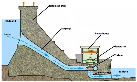
Figure 1. The principle of hydroelectricity.

Water energy resources are potential energy and kinetic energy existing in rivers and are a part of renewable resources, but the reserves of water energy are related to factors such as river flow, evaporation, precipitation, etc. Rivers vary greatly from region to region and climate varies. There is also a large difference in the amount of water energy resources in the region. Due to the current technical conditions, the water volume and the drop of the river part will not be utilized, and the mutual transition between energy also has a certain loss. Therefore, the technically developable hydropower resources are usually lower than their theoretical reserves. Taking the amount of technology developable resources as the basis, the economically available hydropower resources obtained by considering factors such as transmission distance, cost, and flooding loss are smaller than the technically exploitable amount.

Hydropower station reservoirs are generally divided into two categories, one is conventional scheduling and the other is optimized scheduling. Conventional scheduling is a commonly used scheduling method. It can also be called traditional scheduling. It is the most basic adjustment method. It only bases on historical data, no longer considers any other relevant factors, and then uses classical hydraulics and runoff regulation. The scheduling diagram and scheduling rules are used to guide the operation of the reservoir, and the water level of the reservoir is calculated and then expressed as the objective function, that is, the most basic scheduling method is used to ensure the operation of the hydropower station. These schedules are drawn based on past hydrological data and tasks when the reservoir is at different water storage levels, that is, the reservoir scheduling rules when the reservoir is in different states.

The optimal dispatching model of the hydropower station reservoir is based on the optimal theory to establish a mathematical model based on the actual conditions of the hydropower station reservoir, and then using modern computer technology to find the optimal scheduling method that meets the scheduling principle in the process of establishing the optimal scheduling model of the hydropower station. In addition, there are many factors to be considered, including the connection between water and electricity as well as numerous constraints on cascade water inventory, This will minimize pollution in terms of ecological environment, and maximize profits and social benefits in terms of economic benefits. In order to meet the above requirements to the maximum extent and to minimize the water abandonment of hydropower stations, this paper establishes a short-term power generation model suitable for the optimal operation of cascade hydropower stations.

2.2. Maximum Short-Term Generation Model

With the completion and operation of a large number of hydropower stations, the effective solution of large-scale reservoir group optimization scheduling models has become an urgent problem to be solved. The reservoir optimization problem proposes a higher solution quality and running speed for the meta heuristic algorithm. Therefore, this paper proposes a new algorithm called CPIO. This aspect of research not only improves the speed of the operation, but also ensures that the quality of the solution is not worse than the original algorithm and can suppress the premature phenomenon.

Under the given inner diameter flow of the control period, the objective function of the long-term optimal scheduling model of the cascade hydropower station group is defined as: The maximum amount of cascade power generation under the condition of ensuring the output of the cascade is considered during the control period. Under the premise of satisfying the actual situation, this paper selects the maximum benefit of cascade power generation as one of the objective functions. At the same time, it is necessary in the medium and long-term optimization scheduling, it is necessary to consider the output of the period with the least output during the year as much as possible. Medium and long-term optimized dispatching provides the largest possible uniform and reliable output for the power grid, giving full play to the capacity benefits of hydropower generation which can replace thermal power.

$$E=maxF=max\sum _{i=1}^N\sum _{j=1}^{T}A\times q\times \Delta h\times \Delta t$$

(1)

In the formula, A, q, $\Delta h$, $\Delta t$ represents the output coefficient, the outflow rate, the upstream and downstream water level difference respectively. In addition, unit time E is the maximum annual power generation benefit of the cascade hydropower station, N is the total number of cascade hydropower stations, and T is within one year. Calculate the total number of time slots $(T=12)$.

In the process of optimizing the power generation of cascade hydropower stations, it is necessary to understand the water reservoir data in order to first calculate the reservoir upstream capacity and the outflow flow value, and then calculate the downstream water level value based on the outflow flow value.

$$V_{i,j}=\frac{c_1+h_{i,j}^1-c_2}{c_3-c_4}\ast (c_5-c_6)\ast {10}^8$$

(2)

In the formula $c_1$, $c_2$, $c_3$, $c_4$, $c_5$, $c_6$ are a set of variable constants. This set of constants has different values according to the water level in each interval, and $h_{i,j}^1$ is the upstream water level value of the j-th time period of the i-th hydropower station.

$$q_{i,j}=h_j^o-\frac{V_{i,j+1}-V_{i,j}}{t_j\ast 3600}$$

(3)

In the Equation (3), $q_{i,j}$ is the outflow of the j-th time period of the i-th hydropower station, $h_j^o$ is the initial flow of the j-th hydropower station, and $t_j$ is the number of hours of the j-th time period.

$$h_{i,j}^2=\frac{c_7+(q_{i,j}-c_8)}{c_9-c_{10}}\ast (c_{11}-c_{12})$$

(4)

In this Equation (4), $c_7$, $c_8$, $c_9$, $c_{10}$, $c_{11}$, $c_{12}$ are a set of variable constants. This set of constants has different values according to the water level in each interval, and $h_{i,j}^2$ is the downstream water level value of the j-th time period of the i-th hydropower station.

$$\Delta h_i=\frac{h_{i,j}^1+h_{i+1,j}^1}{2}-h_{i,j}^2$$

(5)

In the Equation (5), $\Delta h_i$ is the upstream and downstream water level difference of the i-th hydropower station. When the upstream and downstream water level difference is obtained, since the upstream water level is greatly affected, the average value of the upstream water level is selected for calculation in this paper.

Let us introduce the constraints of the objective function:

$$h_{i,min}\le h_{i,j}\le h_{i,max}$$

(6)

The level of the water level needs to be limited between $h_{min}$ and $h_{max}$.

$$q_{i,min}\le q_{i,j}\le q_{i,max}$$

(7)

The outflow of the reservoir must fluctuate between $q_{min}$ and $q_{max}$. In order to ensure the stable operation of the power generation of the entire cascade hydropower station, the output of the power has to be relatively stable, so the outflow of the reservoir cannot be lower than the minimum flow. In addition, in order to stabilize the life of the turbine and generator, the outflow of the reservoir cannot be higher than the maximum flow.

$$V_{i,min}\le V_{i,j}\le V_{i,max}$$

(8)

The capacity of the reservoir should fluctuate between the $V_{min}$ and $V_{max}$. In order to ensure that the reservoir will continue to work under special circumstances, the reservoir’s capacity cannot be lower than the originally set value to ensure the safe operation and that the downstream organisms are safe, so the capacity cannot be higher than the maximum reservoir capacity.

3. Pigeon-Inspired Optimization

Without prejudice, the minimization problem of the objective function $f\left(x\right)$ is discussed in this paper, where x is the vector that defines the n design variables in the domain D in the decision space.

The pigeon-inspired optimization is a meta-heuristic algorithm that is inspired by the behavior of the pigeons returning home and is widely used in most continuous or discrete optimization problems. This article mainly introduces continuity problems. Referring to extensive literature reviews, a group of pigeons move in decision space D according to the update rules to find the optimal value when looking for the solution of the problem. More formally, in order to gain the satisfactory value of the objective function $f\left(x\right)$, the population of the pigeons is randomly sprinkled in the previously set search space. The objective function judges the equivalent quality of solution based on the position information of each pigeon. At any stage t, the i-th pigeon has its own position vector $x_k^t$ and velocity vector $v_k^t$. For each pigeon, the best solution is the value of the objective function. The best position of the position where the pigeon has passed will be stored. The global optimal solution is continuously updated. To transition from the t step to the $t+1$ step, a more competitive solution will be taken, and each particle is perturbed according to the following formula:

$$v_k^{t+1}=e^{-R\ast t}\ast V_k^t+{\varphi }_1\ast (x_{gbest}-x_k)$$

(9)

and:

$$x_k^{t+1}={\varphi }_2\ast x_k^t+{\varphi }_3\ast v_k^{t+1}$$

(10)

As the formula above suggests, $x_k^t$ refers to the current position of the k-th pigeon, and $x_{gbest}$ is the best position ever found in the entire herd, and the vector $v_k^t$ is a perturbation vector, namely velocity. Finally, ${\varphi }_1$ is a variable constant, is a variable amount limited to 0–1, and ${\varphi }_2$, ${\varphi }_3$ are two weight factors can be constants or variables. This stage belongs to the map and the compass operator. When the pigeon approaches the destination, the dependence on the sun and the magnetic object is reduced, and then the landmark operator is entered.

$$x_{center}^t=\frac{{\sum }_{k=1}^{N^t}{x}_k^t\ast F\left(x_k^t\right)}{N^t\ast {\sum }_{k=1}^{N^t}F\left(x_k^t\right)}$$

(11)

From here on, the landmark operator is entered. In this operator, the pigeons continue to iterate according to the pigeons or landmarks of the roads understood by the population. In the above formula, the purpose of this operation is to find out the pigeons with a high fitness value in the flock. This pigeon is then considered to be the pigeon that knows the road, and the pigeons are iterated according to the pigeon. $N^t$ is the population number at the t-th iteration, and $F\left(X_k^t\right)$ is the fitness function value of the k-th pigeon position.

$$N^t=\frac{N^{t-1}}{2}$$

(12)

The significance of this operation is to halve the pigeons and discard the pigeons that do not have the way to know, to prevent such pigeons from misleading the population into local optimum.

$$x_i^{t+1}=x_i^t+{\varphi }_4\ast (x_{center}^t-x_i^t)$$

(13)

In the formula, ${\varphi }_4$ is a variable constant that value is a randomly generated value from $(0,1)$. In this operation, all pigeons that do not know the road will be iterated according to the pigeons that know the road.

$$F\left(x_i^t\right)=\frac{1}{Fitness\left(x_k^t\right)+\chi }\mathrm{For} \mathrm{minimization} \mathrm{problem}$$

(14)

$$F\left(x_i^t\right)=Fitness\left(x_k^t\right)\mathrm{For} \mathrm{maximization} \mathrm{problem}$$

(15)

For maximizing the problem, OPIO uses Equation (14) to calculate the value of $F\left(x_k^t\right)$ to find the pigeon with the ability to identify the function. For the minimization problem, OPIO uses Equation (15) to calculate the value of $F\left(x_k^t\right)$ to find the pigeon with the function of identifying. In Equation (14), $\chi$ is a non-zero constant whose purpose is to prevent the denominator from being zero.

4. Compact Pigeon-Inspired Optimization

The compact approach replicates the operation of the population-based algorithm by building the probability of a total solution. The optimal process encodes the probability representation of the actual population as a virtual counterpart. Compact pigeon-inspired optimization is a model built on a pigeon-inspired optimization-based framework. In the OPIO algorithm, the concept and design of the CPIO algorithm will be explored in more detail.

The purpose of CPIO is to simulate the operation of OPIO underlying overall algorithm in a smaller version of memory variable memory. By constructing a distributed data structure, the actual solution of the OPIO is transformed into a compact algorithm, the perturbation vector. The PV vector is a probabilistic model for the solution of the population.

$$P{V}^t=[{\mu }^t,{\delta }^t]$$

(16)

In the formula, $\mu$, $\delta$ are two parameters of the standard deviation and the average of the vector $PV$, and t is the current number of iterations. The value of $\mu$, $\delta$ is limited to probability density functions $\left(PDF\right)$ [38] and is changed within [–1, 1]. The magnitude of the PDF is normalized by keeping the area to 1, because by obtaining approximately sufficient in well it is the uniform distribution with a full shape.

The initialization of the virtual population is performed as follows. For each design variable $\mu =0$ and $\delta =\lambda$ , where $\lambda$ is a large constant ($\lambda$ = 10). This value is initialized to initially obtain a normal distribution of truncated wide shapes.

The sampling mechanism of the design variable $x_k^t$ associated with the generic candidate solution x in $PV$ is not a simple process and requires extensive interpretation. For each design variable indexed by k, a truncated Gaussian $PDF$ with the mean $\mu$ and standard deviation $\delta$ is associated, The $PDF$ is described by the following formula:

$$PDF=\frac{e^{-\frac{{(x-\mu \left[k\right])}^2}{2\times \sigma {\left[k\right]}^2}}\times \sqrt{\frac{2}{\pi }}}{\sigma \left[k\right]\times \left(erf(\frac{\mu \left[k\right]+1}{\sqrt{2}\times \sigma \left[k\right]}-erf\left(\frac{\mu \left[k\right]-1}{\sqrt{2}\times \sigma \left[k\right]}\right))\right)}$$

(17)

$PDF$ is the probability distribution function of $PV$, and a truncated Gaussian PDF-related $\mu$, and $\delta$ are formulated. A new candidate solution is generated by iteratively biasing towards a promising region of the optimal solution. Every component of the probability vector may be acquired by learning the previous generations. $erf$ is the error function established by  [39]. $PDF$ corresponds to the cumulative distribution function ($CDF$) by constructing a Chebyshev polynomial [39], and the upper domain of the $CDF$ is randomly changed between 0 and 1. $CDF$ can be described as a real-valued random variable x with a probability distribution, and the value that can be obtained can be less than or equal to $x_k^t$.

The relationship between $CDF$ and $PDF$ can be defined as $CDF={\int }_0^1$PDF$\left(x\right)dx$, and $PV$ operations can sample the design variable $x_k^t$ by randomly generating values within the range of $(0,1)$.

In the iterative process of the compact algorithm, in order to find a better individual, a function that can be compared by two parameters is proposed in this paper. The two variable pigeon parameters are two sample individuals of the $PV$ operation. The vector represented by the winner is the value of the fitness function. This value is higher than other virtual members, and the vector represented by the loser is that the individual fitness value is lower than the fitness evaluation standard. Two variables with return values, the winner and the loser are obtained from the calculation of the objective function, and a new candidate solution is generated to compare with the original global optimal solution to generate new winners and losers. For updating $PV$ operations, $\mu$ and $\sigma$ can be considered for updates according to the rules below. If the mean value of $\mu$ is 1, Then the update rule becomes ${\mu }^t$ and ${\sigma }^t$ for each of its elements ${\mu }^{t+1}$ and ${\sigma }^{t+1}$ [40] as described in the following:

$${\mu }_i^{t+1}={\mu }_i^t+\frac{winne{r}_i-lose{r}_i}{N},$$

(18)

where N is the virtual population size and the value of $\delta$ is described below. The update rule for each element is given in the formula below.

$${\sigma }_i^{t+1}=\sqrt{{\left({\sigma }_i^t\right)}^2+{\left({\mu }^{t+1}\right)}^2+\frac{winne{r}_i^2-lose{r}_i^2}{N}}$$

(19)

Mathematical details about construction Equations (18) and (19) have been given. The persistent and non-persistent structures of rcGA have been tested and can be seen in [41]. Seeing the virtual population size N as a parameter of a compression algorithm is not a true population-based algorithm. The virtual population size, in the real-valued compression algorithm, is an algorithm that depends on the convergence speed.

In general, a probabilistic model for compact OPIO is hired to represent all of the set of solutions for the pigeon group, neither storing location information nor storing speed information; however, storing newly generated candidate solutions. Therefore, the limited storage space is required to achieve the algorithm requirements which saves a lot of time and hardware resources for the cascade hydropower station to optimize the short-term power generation model.

CPIO uses a perturbation vector $PV$ that has the same structure as the one shown in Equation (16), at the beginning of the optimization algorithm, just like the process described in Equation (17). The $PV$ initialization is designed as $(\forall k,\mu [k]=0,\sigma [k]=\lambda ,\lambda =10)$ and the variables of each design are limited to one continuous space $[-1,1]$, and in addition, the position x and the velocity v are randomly initialized within a certain range.

Update velocity vector and position vector by slightly revised pigeon-inspired algorithm:

$$v_k^{t+1}={\omega }_1\ast e^{-R\ast t}\ast V_k^t+{\omega }_2\ast (x_{gbest}-x_k)$$

(20)

and:

$$x_k^{t+1}={\xi }_1\ast x_k^t+{\xi }_2\ast v_k^{t+1}$$

(21)

${\omega }_1$ is an inertia weight, ${\omega }_2$ is a random variable between 0 and 1, and ${\xi }_1$ and ${\xi }_2$ are weighting factors that control the position update of the pigeon.

It can be seen that the equation updating of speed (Equation (20)) and position (Equation (21)) is similar to the OPIO algorithm. In the original version, pigeon k was closely related to pigeon group N. In the compact version, there was no real population, but the relevance of a virtual population pigeon to the virtual population was not that great. It is easy to see that compact OPIO is just a pigeon that uses the update formula to update it, so updating it once produces a solution that saves a lot of memory.

In the landmark operator entering the second stage of CPIO, the original algorithm uses the Equation (11) to determine the pigeon with the function of identifying the function based on the fitness solution of each pigeon position, so that it becomes the center point and continues to update. Since the CPIO has only one particle to update, it is not suitable when selecting a pigeon with a path function. In this paper, a center point suitable for CPIO is proposed. By setting a virtual center position point, the guiding pigeon is updated. When the virtual center position is established, it is based on the historical fitness value of the pigeon. The number selected is also based on the size of the virtual population.

$$x_{center}^{t+1}=\frac{{\sum }_{i=l-N+1}^{N}F\left(x_k^t\right)}{N}$$

(22)

l is the number of iterations until now, N is the number of virtual populations. According to the Equation (22), the historical virtual center points of the pigeons can be selected, and it is known that they continue to iterate.

$$x_k^{t+1}=x_k^t+{\omega }_3\ast (x_{center}^t-x_k^t)$$

(23)

It is easy to see that CPIO saves a lot of memory space, so this approach can be applied to other variations of OPIO.

5. Numerical Results

The test results of the CPIO that have been tested by 29 test functions, and these test functions come from [42]. Each test function has a very detailed introduction in Table 1 and Table 2. Among these groups of questions, they have different search range and different expressions.

Table 1. Details of 29 test functions.

Name	Test Functions	Range	Global Minimum
Sphere	$f\left(x\right)={\sum }_{i=1}^d{x}_i^2$	$\pm 5.12$	0
Rastrigin	$f\left(x\right)=10d+{\sum }_{i=1}^d[x_i^2-10\ast cos\left(2\pi x_i\right)]$	$\pm 5.12$	0
Rosenbrock	$f\left(x\right)={\sum }_{i=1}^{d-1}[100\ast (x_{i+1}-x_i^2)+{(x_i-1)}^2]$	$x_i\in [-5,10]$	0
Griewank	$f\left(x\right)={\sum }_{i=1}^d\frac{x_i^2}{4000}-{\prod }_{i=1}^{d}cos\left(\frac{x_i}{\sqrt{i}}\right)+1$	$\pm 600$	0
Ackley	$f\left(x\right)=-a\ast exp(-b\sqrt{\frac{{\sum }_{i=1}^d{x}_i^2}{d}})$ $-exp\left(\frac{{\sum }_{i=1}^{d}cos\left(c{x}_i\right)}{d}\right)+a+exp\left(l\right)$	$\pm 32.768$	0
Quadric	$f\left(x\right)={\sum }_{i=1}^n{\sum }_{k=1}^i{x}_i$	$\pm 32.768$	0
Bukin6	$f\left(x\right)=100\ast \sqrt{\left|x_2-0.01\ast x_1^2\right|}+0.01\ast \left|x_1+10\right|$	$x_1\in [-15,5]x_2\in [-3,3]$	0
Crossit	$f\left(x\right)=-0.0001\ast$ ${\left(\left|sin\left(x_1\right)sin\left(x_2\right)\ast exp\left(\left|100-\frac{\sqrt{x_1^2+x_2^2}}{\pi }\right|\right)+1\right|\right)}^{0.1}$	$\pm 10$	−2.06261
Drop	$f\left(x\right)=-\frac{1+cos\left(12\sqrt{x_1^2+x_2^2}\right)}{0.5(x_1^2+x_2^2)+2}$	$\pm 5.12$	−1
Egg	$f\left(x\right)=-(x_2+47)\ast sin\left(\sqrt{\left|x_2+\frac{x_1}{2}+47\right|}\right)$ $-x_1\ast sin\left(\left|x_1-(x_2+47)\right|\right)$	$\pm 512$	−959.6407
Holder	$f\left(x\right)=-\left|sin\left(x_1\right)cos\left(x_2\right)exp\left(\left|1-\frac{\sqrt{x_1^2+x_2^2}}{\pi }\right|\right)\right|$	$\pm 10$	−19.2085
Levy	$f\left(x\right)=si{n}^2\left(\pi w_1\right)$ $+{\sum }_{i=1}^{d-1}{(w_i-1)}^2\left[1+10si{n}^2(\pi w_i+1)\right]$ $+{(w_d-1)}^2\left[1+si{n}^2\left(2\pi w_d\right)\right]$	$\pm 10$	−19.2085
Levy13	$f\left(x\right)=si{n}^2\left(3\pi w_1\right)+{(x_1-1)}^2[1+si{n}^2\left(3\pi x_2\right)]$ $+{(x_2-1)}^2[1+si{n}^2\left(2\pi x_2\right)])$	$\pm 10$	0
Schaffer2	$f\left(x\right)=0.5+\frac{si{n}^2(x_1^2-x_2^2)-0.5}{[1+0.001(x_1^2+x_2^2)]}$	$\pm 100$	0

Table 2. Details of 29 test functions.

Name	Test Functions	Range	Global Minimum
Schaffer4	$f\left(x\right)=0.5+\frac{cos\left(sin\left(\left|x_1^2-x_2^2\right|\right)\right)-0.5}{[1+0.001(x_1^2+x_2^2)]}$	$\pm 100$
Schwef	$f\left(x\right)=418.9829d-{\sum }_{i=1}^d{x}_{i}sin\left(\sqrt{\left|x_i\right|}\right)$	$\pm 500$	0
Shubert	$f\left(x\right)=\left({\sum }_{i=}^{5}icos\left((i+1)\right)\right)({\sum }_{i=1}^{5}icos(i+1)x_2+i)$	$\pm 5.12$	−186.7309
Boha1	$f\left(x\right)=x_1^2+2x_2^2-0.3cos\left(3\pi x_1\right)-0.4cos\left(4\pi x_2\right)+0.7$	$\pm 100$	0
Perm0db	$f\left(x\right)={\sum }_{i=1}^d\left({\sum }_{j=1}^d(j+\beta )(x_j^i-\frac{1}{j^i})\right)$	$\pm 30$	0
Rothyp	$f\left(x\right)={\sum }_{i=1}^d{\sum }_{j=1}^i{x}_j^2$	$\pm 65.536$	0
Sumpow	$f\left(x\right)={\sum }_{i=1}^d{\left|x_i\right|}^{i+1}$	$x_i\in [-1,1]$	0
Sumsqu	$f\left(x\right)={\sum }_{i=1}^{d}i{x}_i^2$	$\pm 10$	0
Trid	$f\left(x\right)={\sum }_{i=1}^d{(x_i-1)}^2-{\sum }_{i=2}^d{x}_i{x}_{i-1}$	$\pm 30$	0
Booth	$f\left(x\right)={(x_1+2x_2-7)}^2+{(2x_1+x_2-5)}^2$	$\pm 10$	0
Matya	$f\left(x\right)=0.26(x_1^2+x_2^2)-0.48x_1{x}_2$	$\pm 10$	0
Mccorm	$f\left(x\right)=sin(x_1+x_2)+{(x_1-x_2)}^2-1.5x_1+2.5x_2+1$	$x_1\in [-1.5,4]x_2\in [-3,4]$	−1.9133
Camel3	$f\left(x\right)=2x_1^2-1.05x_1^4+\frac{x_1^6}{6}+x_1{x}_2+x_2^2$	$\pm 5$	0
Beale	$f\left(x\right)={\left(1.5-x_1+x_1{x}_2\right)}^2$ $+{\left(2.25-x_1+x_1{x}_2^2\right)}^2$ $+{\left(2.625-x_1+x_1{x}_2^3\right)}^2$	$\pm 4.5$	0
Stybtang	$f\left(x\right)=\frac{1}{2}\ast {\sum }_{i=1}^d(x_i^4-16x_i^2+5x_i)$	$\pm 5$	−1174.9797

In Equations (20)–(23) and Algorithm 1, the parameters of the CPIO proposed herein are: $N=120,R=0.2$. The values of these parameters are referred to [43] and have a slight change. More specifically, in order to make CPIO work better, we modeled the virtual population size proposed by OPIO. In this article, CPIO is compared to the OPIO. In all test functions, CPIO is run 30 times and averaged. Take the minimum value of CPIO in all test functions.

Algorithm 1 Compact pigeon-inspired optimization (CPIO) pseudo-code.

1: Map and compass factors R, The maximum number of iterations in the first stage $MaxD{T}_1$ and The maximum number of iterations in the second stage $MaxD{T}_2$, dimension is $dim$; 2: for$k=1$ to $dim$ do 3:     $//$ $PV$ operation initialization; N is the total number of pigeons 4:     initialize $\mu \left[k\right]=0$ 5:     initialize $\sigma \left[k\right]=10$ 6: end for 7: $//$ Global Best initialization 8: Generate the global best solution $x_{best}$ by means of perturbation vector $PV$ 9: $//$ Local Best Solution initialization 10: Generate the local best solution $x_k$ by $PV$ 11: for$t=1$ to $MaxD{t}_1$ do 12:     $x_k^t=$ Generate from $PV$ operation 13:     $//$ Update position and velocity 14:     $v_k^{t+1}={\omega }_1\ast e^{-R\ast t}\ast V_k^t+{\omega }_2\ast (x_{gbest}-x_k)$ 15:     $x_k^{t+1}={\xi }_1\ast x_k^t+{\xi }_2\ast v_k^{t+1}$ 16:     $//$ Best Selection 17:     $[winner,loser]$=compete($x_k^{t+1},x_{gbest}$) 18:     $//$ Update $PV$ operation 19:     for $k=1:dim$ do 20:         ${\mu }^{t+1}\left[k\right]={\mu }^t\left[k\right]+\frac{winner\left[k\right]-loser\left[k\right]}{N}$ 21:         ${\sigma }^{t+1}\left[k\right]=\sqrt{{\left({\sigma }^t\left[k\right]\right)}^2+{\left({\mu }^t\left[k\right]\right)}^2-{\left({\mu }^{t+1}\left[k\right]\right)}^2+\frac{winne{r}_k^2-lose{r}_k^2}{N}}$ 22:     end for 23: end for 24: for$t=MaxD{t}_1+1$ to $MaxD{t}_1+MaxD{t}_2$ do 25:     $//$ Enter the second stage 26:     $//$ Select the virtual center pigeon from the historical best points 27:     $x_k^{t+1}=x_k^t+{\omega }_3\ast (x_{center}^t-x_k^t)$ 28:     $//$ Best Selection 29:     $[winner,loser]$=compete($x_k^{t+1},x_{gbest}$) 30:     $//$ Update $PV$ operation 31:     for $i=1:dim$ do 32:         ${\mu }^{t+1}\left[k\right]={\mu }^t\left[k\right]+\frac{winner\left[k\right]-loser\left[k\right]}{N}$ 33:         ${\sigma }^{t+1}\left[k\right]=\sqrt{{\left({\sigma }^t\left[k\right]\right)}^2+{\left({\mu }^t\left[k\right]\right)}^2-{\left({\mu }^{t+1}\left[k\right]\right)}^2+\frac{winne{r}_k^2-lose{r}_k^2}{N}}$ 34:     end for 35: end for

When initializing the two algorithms CPIO and original pigeon-inspired optimization (OPIO) , the map and compass factor R are set to 0.2, and the result is to compare CPIO and OPIO. The quality of solution and the number of runs of CPIO and OPIO optimal solutions are compared as below described. The CPIO and OPIO data results are the average of 30 runs. All algorithms operate 500 times, including 300 in the first phase and 200 in the second phase.

In Table 3, CPIO performs better than OPIO in many test functions, and most of the values perform well. In terms of the time cost comparison, it is easy to see that CPIO time spent is much better than PIO, especially in several of them, and the time spent is more than a hundred times more.

Table 3. Comparison, evaluation and speed of quality performance between CPIO and OPIO.

Test Functions	Fitness Function Value		Time
	CPIO	OPIO	CPIO	OPIO
Sphere	$1.96\times {10}^{-1}$	$2.09\times {10}^0$	1.62 $\times {10}^{-1}$	$4.23\times {10}^{-1}$
Rastrigin	$2.13\times {10}^1$	$4.42\times {10}^1$	$1.37\times {10}^{-1}$	$7.92\times {10}^{-1}$
Rosenbrock	$4.45\times {10}^1$	$7.92\times {10}^1$	$1.35\times {10}^{-1}$	$7.50\times {10}^{-1}$
Griewank	$5.51\times {10}^{-5}$	$1.04\times {10}^{-1}$	$1.67\times {10}^{-1}$	$1.15\times {10}^0$
Ackley	$5.93\times {10}^{-1}$	$2.43\times {10}^0$	$1.88\times {10}^{-1}$	$1.23\times {10}^1$
Quadric	$6.50\times {10}^{-1}$	$2.5\times {10}^1$	$1.84\times {10}^{-1}$	$1.03\times {10}^1$
Bukin6	$1.96\times {10}^0$	$6.24\times {10}^0$	$1.40\times {10}^{-1}$	$6.06\times {10}^{-1}$
Crossit	$-2.06\times {10}^0$	$-2.06\times {10}^0$	1.57$\times {10}^{-1}$	$8.48\times {10}^{-1}$
Drop	$-9.86\times {10}^{-1}$	$-9.36\times {10}^{-1}$	$1.48\times {10}^{-1}$	$7.93\times {10}^{-1}$
Egg	$-5.49\times {10}^1$	$-9.36\times {10}^{-1}$	$1.49\times {10}^{-1}$	$8.36\times {10}^{-1}$
Holder	$-1.73\times {10}^0$	$-1.73\times {10}^0$	$1.46\times {10}^{-1}$	$7.77\times {10}^{-1}$
Levy	$3.58\times {10}^{-1}$	$1.27\times {10}^{-1}$	$1.58\times {10}^{-1}$	$4.00\times {10}^0$
Levy13	$1.51\times {10}^{-1}$	$1.35\times {10}^{-31}$	$1.54\times {10}^{-1}$	$5.47\times {10}^{-1}$
Schaffer2	$3.12\times {10}^{-8}$	0	$1.63\times {10}^{-1}$	$5.18\times {10}^{-1}$
Schaffer4	$6.39\times {10}^{-1}$	$5.40\times {10}^{-1}$	$1.47\times {10}^{-1}$	$5.26\times {10}^{-1}$
Schwef	$-7.71\times {10}^{96}$	$1.25\times {10}^4$	$1.75\times {10}^{-1}$	$1.13\times {10}^0$
Shubert	$-1.57\times {10}^2$	$-7.45\times {10}^0$	$1.49\times {10}^{-1}$	$6.31\times {10}^{-1}$
Boha1	$1.92\times {10}^{-4}$	$3.33\times {10}^{-17}$	$1.61\times {10}^{-1}$	$4.82\times {10}^{-1}$
Perm0db	$2.24\times {10}^{-4}$	0	$1.60\times {10}^{-1}$	$4.76\times {10}^{-1}$
Rothyp	$3.24\times {10}^3$	$4.33\times {10}^3$	$4.10\times {10}^{-1}$	$7.80\times {10}^0$
Sumpow	$2.58\times {10}^0$	$2.84\times {10}^1$	$1.45\times {10}^{-1}$	$2.37\times {10}^0$
Sumsqu	$2.05\times {10}^{-6}$	$9.14\times {10}^{-3}$	$1.70\times {10}^{-1}$	$1.74\times {10}^0$
Trid	$3.08\times {10}^0$	$2.37\times {10}^1$	$1.39\times {10}^{-1}$	$6.03\times {10}^{-1}$
Booth	$-2.21\times {10}^2$	$-2.90\times {10}^1$	$1.47\times {10}^{-1}$	$6.92\times {10}^{-1}$
Matya	$1.51\times {10}^0$	$2.97\times {10}^{-1}$	$1.53\times {10}^{-1}$	$4.54\times {10}^{-1}$
Mccorm	$1.80\times {10}^{-6}$	$7.74\times {10}^{-11}$	$1.59\times {10}^{-1}$	$4.43\times {10}^{-1}$
Camel3	$-1.79\times {10}^0$	$-1.90\times {10}^0$	$1.57\times {10}^{-1}$	$4.56\times {10}^{-1}$
Beale	$8.34\times {10}^{-6}$	$5.35\times {10}^{-25}$	$1.61\times {10}^{-1}$	$5.58\times {10}^{-1}$
Stybtang	$2.77\times {10}^0$	$5.71\times {10}^{-2}$	$1.53\times {10}^{-1}$	$5.34\times {10}^{-1}$

According to the comparison of the two algorithms, it can be concluded that the running time of CPIO is much lower than that of the original algorithm. This is because the number of population used in the process of iteration is different. In the new algorithm, it uses an example to keep iterating, constantly adjusting the probability distribution according to the path that has been iterated, and the greater the possibility of generating particles where the function values are superior. However, this method also has a big problem, since in the search process of a single particle, randomness is often large, and it is thus easy to fall into the local optimal. It is also relatively simple to achieve the optimal, in the case of small dimension settings, the advantages of the algorithm are not obvious. Because of this characteristic of the new algorithm, it is easy to save time and reduce the time complexity of the algorithm.

Figure 2 shows the convergence trend of CPIO and OPIO. Best score obtained so far refers to the optimal value obtained by the algorithm during the iteration process. While the convergence speed of OPIO and the algebra needed to achieve optimal are small, the optimal value of CPIO is better or nearly equal to the value of OPIO. Here, CPIO uses one particle for updating and iteration, while OPIO uses the entire population for optimization. CPIO is far less than OPIO search capability, but CPIO can save a lot of memory and time to find excellence.

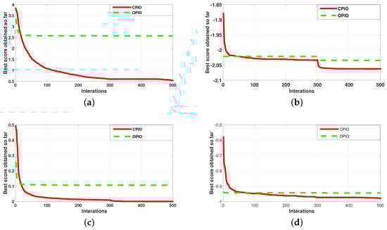
Figure 2. Compact pigeon-inspired optimization (CPIO) and original pigeon-inspired optimization (OPIO) performance in test functions. (a) Ackley; (b) Crossit; (c) Drop; (d) Griewank.

Among the four selected functions, Figure 3 shows the time trend of the four functions running 30 times. In general, the time spent by the CPIO and PIO algorithms does not change much, but the two algorithms compare. It is easy to see that CPIO runs much faster than the PIO.

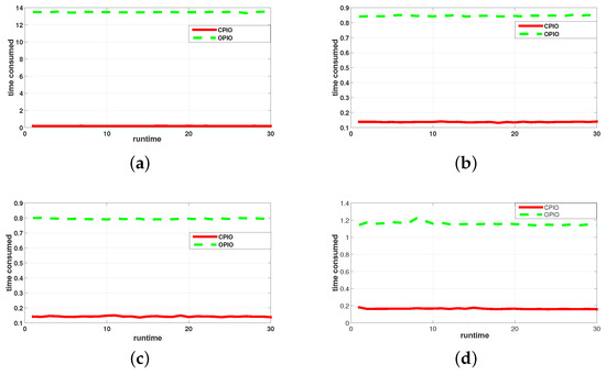
Figure 3. CPIO and OPIO performance in test functions. (a) Ackley; (b) Crossit; (c) Drop; (d) Griewank.

Table 4 shows the comparison of CPIO and PIO mentioned above in the memory variables, which makes it very convenient to implement the calculation algorithm. The number of variables of the two algorithms of CPIO and PIO proposed in this paper is calculated by the equation used in the computational optimization. In Table 4, it is easy to see that in the same computing situation, CPIO uses less memory than PIO. For example, during an iteration, CPIO uses an iteration Equations (16)–(23); the formula for PIO update iteration is Equations (9)–(13).

Table 4. The space complexity of the two algorithms.

Algorithm	Particle	Memory Size	Computing Complexity	Use Equations
CPIO	1	8	$8\times T\times iteration$	(16), (17), (18), (19), (20), (21), (22), (23)
OPIO	N	$5\times N$	$5\times T\times N\times iteration$	(9), (10), (11), (12), (13)

As can be seen from Table 4, the actual population size of the PIO is N, but the actual population size in the CPIO is 1, and the virtual population number is N. In the case where the number of iterations l and the running time t are the same, the memory usage of the variables of OPIO and CPIO is iterated by $4\times t\times N$ and $8\times t$, respectively. Here, it is seen that the memory occupancy of the PIO is larger than the memory usage of the CPIO.

In Figure 4, the consequence of the presented algorithm and the else three meta-heuristics are shown. According to Table 5, the trend and optimal value of CPIO are fundamentally better than the other three algorithms, and have a superior performance. Table 5 shows the comparison of CPIO, OPIO and other algorithms, such as CPSO and PSO algorithms. Among the four meta-heuristic algorithms, the performance is as follows in 29 test functions. In the process of algorithm simulation, as part of the images are not so obvious, four relatively obvious images are extracted for display.

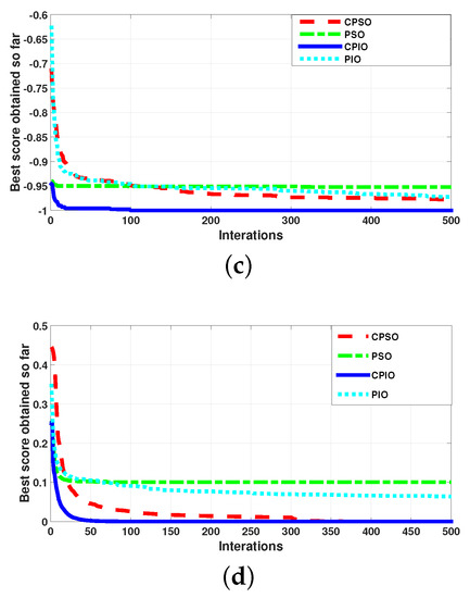
Figure 4. CPIO and three other meta-heuristic algorithms for testing function performance. (a) Ackley; (b) Crossit; (c) Drop; (d) Griewank.

Table 5. The optimal value and time cost of the four algorithms.

Test Functions	Fitness Function Value				Time
	CPIO	OPIO	PSO	CPSO	CPIO	OPIO	PSO	CPSO
Sphere	$5.16\times {10}^{-1}$	$9.79\times {10}^{-1}$	$3.73\times {10}^{-6}$	$4.69\times {10}^0$	$1.45\times {10}^{-1}$	$4.50\times {10}^0$	$9.94\times {10}^0$	$1.70\times {10}^0$
Rastrigin	$1.95\times {10}^2$	$1.68\times {10}^1$	$2.56\times {10}^1$	$2.14\times {10}^2$	$1.40\times {10}^{-1}$	$4.54\times {10}^0$	$1.63\times {10}^1$	$1.71\times {10}^{-1}$
Rosenbrock	$1.40\times {10}^2$	$7.21\times {10}^2$	$2.13\times {10}^4$	$4.68\times {10}^2$	$1.38\times {10}^{-1}$	$4.52\times {10}^0$	$1.21\times {10}^1$	$1.71\times {10}^{-1}$
Griewank	$9.53\times {10}^{-6}$	$1.78\times {10}^1$	$4.25\times {10}^2$	$1.38\times {10}^{-1}$	$1.14\times {10}^{-1}$	$4.42\times {10}^0$	$2.26\times {10}^1$	$8.34\times {10}^{-2}$
Ackley	$1.11\times {10}^0$	$3.12\times {10}^0$	$3.95\times {10}^0$	$3.12\times {10}^0$	$2.51\times {10}^{-1}$	$7.22\times {10}^0$	$1.97\times {10}^2$	$2.30\times {10}^{-1}$
Quadric	$1.49\times {10}^0$	$3.25\times {10}^0$	$2.89\times {10}^0$	$2.99\times {10}^0$	$2.30\times {10}^{-1}$	$7.22\times {10}^0$	$1.98\times {10}^2$	$2.29\times {10}^{-1}$
Bukin6	$3.66\times {10}^0$	$4.28\times {10}^{-2}$	$3.72\times {10}^{-2}$	$3.36\times {10}^0$	$1.41\times {10}^{-1}$	$4.47\times {10}^0$	$1.44\times {10}^1$	$1.67\times {10}^{-1}$
Crossit	−$2.06\times {10}^0$	−$2.06\times {10}^0$	−$2.06\times {10}^0$	−$2.06\times {10}^0$	$1.58\times {10}^{-1}$	$4.48\times {10}^0$	$1.67\times {10}^1$	$1.74\times {10}^{-1}$
Drop	−$9.76\times {10}^{-1}$	−$9.58\times {10}^{-1}$	−$9.93\times {10}^{-1}$	−$9.44\times {10}^{-1}$	$1.51\times {10}^{-1}$	$4.50\times {10}^0$	$1.60\times {10}^1$	$1.68\times {10}^{-1}$
Egg	−$3.85\times {10}^2$	−$8.90\times {10}^2$	−$9.15\times {10}^2$	−$5.80\times {10}^7$	$1.58\times {10}^{-1}$	$4.31\times {10}^0$	$1.64\times {10}^1$	$1.14\times {10}^{-1}$
Holder	−$6.24\times {10}^1$	−$1.92\times {10}^1$	−$1.92\times {10}^1$	−$1.92\times {10}^1$	$2.91\times {10}^{-2}$	$4.53\times {10}^{-1}$	$1.08\times {10}^0$	$3.42\times {10}^{-2}$
Levy	$1.78\times {10}^{-3}$	$1.22\times {10}^{-30}$	$1.50\times {10}^{-32}$	$1.30\times {10}^{-3}$	$4.07\times {10}^{-2}$	$5.93\times {10}^{-1}$	$2.12\times {10}^0$	$3.45\times {10}^{-2}$
Levy13	$7.49\times {10}^{-2}$	$2.39\times {10}^{-19}$	$1.35\times {10}^{-31}$	$6.53\times {10}^{-2}$	$2.56\times {10}^{-2}$	$3.98\times {10}^{-1}$	$8.40\times {10}^{-1}$	$2.60\times {10}^{-2}$
Schaffer2	$4.00\times {10}^{-9}$	$1.42\times {10}^{-3}$	0	$1.65\times {10}^{-4}$	$2.60\times {10}^{-2}$	$4.09\times {10}^{-1}$	$7.90\times {10}^{-1}$	$2.17\times {10}^{-2}$
Schaffer4	$5.09\times {10}^{-1}$	$5.00\times {10}^{-1}$	$5.00\times {10}^{-1}$	$5.00\times {10}^{-1}$	$2.95\times {10}^{-2}$	$4.07\times {10}^{-1}$	$7.63\times {10}^{-1}$	$3.25\times {10}^{-2}$
Schwef	$1.44\times {10}^3$	$9.30\times {10}^4$	$9.26\times {10}^4$	$1.40\times {10}^3$	$1.69\times {10}^{-1}$	$4.39\times {10}^0$	$2.15\times {10}^1$	$1.03\times {10}^{-1}$
Shubert	−$1.47\times {10}^2$	−$1.86\times {10}^2$	−$1.86\times {10}^2$	−$1.36\times {10}^2$	$2.62\times {10}^{-2}$	$4.09\times {10}^{-1}$	$8.83\times {10}^{-1}$	$2.64\times {10}^{-2}$
Boha1	$4.14\times {10}^{-4}$	0	0	$2.24\times {10}^{-1}$	$2.38\times {10}^{-2}$	$3.95\times {10}^{-1}$	$7.87\times {10}^{-1}$	$2.05\times {10}^{-2}$
Perm0db	$4.69\times {10}^{-1}$	$5.04\times {10}^2$	$1.24\times {10}^3$	$1.67\times {10}^2$	$1.91\times {10}^{-1}$	$4.07\times {10}^0$	$7.78\times {10}^1$	$1.59\times {10}^{-1}$
Rothyp	$1.69\times {10}^1$	$5.64\times {10}^4$	$4.82\times {10}^4$	$7.19\times {10}^1$	$1.44\times {10}^{-1}$	$4.78\times {10}^0$	$4.02\times {10}^1$	$1.34\times {10}^{-1}$
Sumpow	$1.19\times {10}^{-5}$	$1.87\times {10}^{-1}$	$1.64\times {10}^{-1}$	$4.71\times {10}^{-1}$	$1.79\times {10}^{-1}$	$4.49\times {10}^0$	$3.04\times {10}^1$	$1.79\times {10}^{-1}$
Sumsqu	$1.52\times {10}^1$	$5.80\times {10}^2$	$6.94\times {10}^3$	$5.3\times {10}^1$	$1.41\times {10}^{-1}$	$4.26\times {10}^0$	$1.28\times {10}^1$	$1.71\times {10}^{-1}$
Trid	−$8.08\times {10}^0$	−$7.35\times {10}^0$	−$1.99\times {10}^2$	−$2.88\times {10}^1$	$5.20\times {10}^{-2}$	$1.55\times {10}^0$	$4.03\times {10}^0$	$4.41\times {10}^{-2}$
Booth	$9.31\times {10}^{-1}$	$1.31\times {10}^{-3}$	0	$1.45\times {10}^1$	$2.44\times {10}^{-2}$	$3.82\times {10}^{-1}$	$6.90\times {10}^{-1}$	$2.31\times {10}^{-2}$
Matya	$2.97\times {10}^{-1}$	$1.51\times {10}^0$	$1.67\times {10}^0$	$9.72\times {10}^{-1}$	$1.53\times {10}^{-1}$	$4.51\times {10}^{-1}$	$7.56\times {10}^0$	$1.75\times {10}^{-1}$
Mccorm	−$1.82\times {10}^0$	−$1.81\times {10}^0$	−$1.83\times {10}^0$	−$1.64\times {10}^0$	$2.90\times {10}^{-2}$	$3.85\times {10}^{-1}$	$6.72\times {10}^{-1}$	$2.58\times {10}^{-2}$
Camel3	$8.12\times {10}^{-6}$	$1.29\times {10}^{-1}$	$2.80\times {10}^{-1}$	$4.41\times {10}^{-1}$	$2.79\times {10}^{-2}$	$3.88\times {10}^{-1}$	$7.88\times {10}^{-1}$	$2.69\times {10}^{-2}$
Beale	$1.89\times {10}^0$	$6.78\times {10}^{-1}$	$5.10\times {10}^{-1}$	$8.17\times {10}^0$	$2.55\times {10}^{-2}$	$3.77\times {10}^{-1}$	$7.66\times {10}^{-1}$	$2.51\times {10}^{-2}$
Stybtang	−$3.18\times {10}^2$	−$2.37\times {10}^2$	−$2.33\times {10}^2$	−$2.81\times {10}^2$	$5.99\times {10}^{-2}$	$1.55\times {10}^0$	$5.42\times {10}^0$	$6.77\times {10}^2$

6. Experiments of Short-Term Power Generation Model for Cascade Hydropower Stations

Wanjiazhai Water Conservancy Project: The Wanjiazhai Water Conservancy Project is located in the canyon of the Tuoketuo to Longkou section of the Yellow River in the north of the Yellow River. It is the first of the eight cascades planned for the development of the middle reaches of the Yellow River. and also the Shanxi Yellow River Diversion Project. The starting point of the project the left bank is affiliated to the Pianguan County of Shanxi Province, and the right bank is subordinate to the Zhungeer Banner of Inner Mongolia Autonomous Region. The dam site controls a drainage area of 395,000 square kilometers, with a total storage capacity of 896 million cubic meters and a storage capacity of 445 million cubic meters. It has comprehensive benefits such as water supply, power generation, flood control and anti-icing.

Longkou Hydropower Station is located at the junction of two provinces, Hequ County, Shanxi Province and Zhungeer Banner, Inner Mongolia. It is $25.6$ km from the upstream Wanjiazhai Water Control Project and 70 km from the downstream Tianqiao Hydropower Station. It is the regional center of energy and chemical bases in Shanxi Province and Inner Mongolia Autonomous Region, and controls the drainage area of $\mathrm{397,406}$ square kilometers.

Table 6 shows the monthly inflow values of the two cascade hydropower stations in the wet years, the flat water years and the dry years. ASP is Annual scheduling period.

Table 6. Cascade hydropower station monthly water supply.

ASP	1	2	3	4	5	6	7	8	9	10	11	12
high flow	149.7	193	176.2	900.1	1077.1	1441.7	343.9	318.1	177.9	36.6	28.6	45.9
median water	82.9	243.9	598.1	554	203.5	146.2	491.7	208.3	147.8	340.9	573.3	104.5
low flow	188.2	251	255.8	550.2	406.6	849.2	132.9	81	59	121.3	11.6	7.8

The short-term power generation model of cascade hydropower stations has been introduced above. Figure 5 showcases the main flow of the algorithm. In this paper, the three periods of the two cascade hydropower stations are scheduled and modeled by Equations (1)–(8) and the sum of the power generation of the two cascade hydropower stations is the largest. As shown in Figure 6, at any stage, CPIO has the largest scheduling capacity for the two cascade hydropower stations, and the total power generation is also relatively huge. CPIO dispatched the two cascade hydropower stations. The final result has the power generation at $3.968\times {10}^{17}$ KWH in the high flow year, and the total power generation at $3.108\times {10}^{17}$ KWH in the year of the median water. The power generation at $2.396\times {10}^{17}$ KWH in the low year.

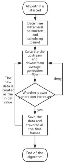
Figure 5. The main process of optimizing hydropower station.

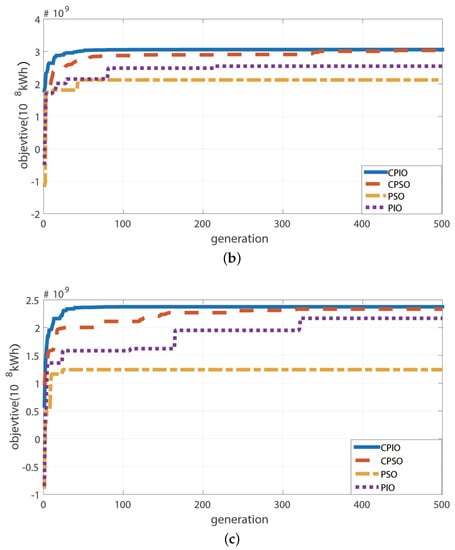
Figure 6. Comparison of four meta-heuristic algorithms in cascade hydropower stations: (a) Wet water years schedule; (b) flat water years schedule; and (c) dry water years schedule.

7. Conclusions

A novel optimization approach called compact pigeon-inspired optimization (CPIO) is proposed. The proposed CPIO was tested on 29 classical test functions to demonstrate the usefulness of the proposed optimization method. A compact method is successfully used in the pigeon-inspired optimization algorithm to reduce the usage of the memory size. The proposed CPIO was also applied to cascade hydroelectric power generation. Simulation results show the CPIO may reach better results compared with some existing algorithms for the cascade hydroelectric power station.

References

- Yang, X.S. Nature-Inspired Metaheuristic Algorithms; Luniver Press: Frome, UK, 2010; pp. 15–35. ISBN 978-1-905986-28-6. [Google Scholar]
- Jia, Z.; Sahmoudi, M. A type of collective detection scheme with improved pigeon-inspired optimization. Int. J. Intell. Comput. Cybern. 2016, 9, 105–123. [Google Scholar] [CrossRef]
- Chen, S.; Duan, H. Fast image matching via multi-scale Gaussian mutation pigeon-inspired optimization for low cost quadrotor. Aircr. Eng. Aerosp. Technol. 2017, 89, 777–790. [Google Scholar] [CrossRef]
- Qiu, H.; Duan, H. Multi-objective pigeon-inspired optimization for brushless direct current motor parameter design. Sci. China Technol. Sci. 2015, 58, 1915–1923. [Google Scholar] [CrossRef]
- Deng, X.W.; Shi, Y.Q.; Li, S.L.; Li, W.; Deng, S.W. Multi-objective pigeon-inspired optimization localization algorithm for large-scale agricultural sensor network. J. Huaihua Univ. 2017, 36, 37–40. [Google Scholar]
- Fu, X.; Chan, F.T.; Niu, B.; Chung, N.S.; Qu, T. A multi-objective pigeon inspired optimization algorithm for fuzzy production scheduling problem considering mould maintenance. Sci. China Inf. Sci. 2019, 62, 70202. [Google Scholar] [CrossRef]
- Pan, J.S.; Kong, L.; Sung, T.W.; Tsai, P.W.; Snášel, V. α-Fraction first strategy for hierarchical model in wireless sensor networks. J. Internet Technol. 2018, 19, 1717–1726. [Google Scholar]
- Wang, J.; Gao, Y.; Liu, W.; Sangaiah, A.K.; Kim, H.J. An intelligent data gathering schema with data fusion supported for mobile sink in wireless sensor networks. Int. J. Distrib. Sens. Netw. 2019, 15, 1550147719839581. [Google Scholar] [CrossRef]
- Wang, L.; Singh, C. Environmental/economic power dispatch using a fuzzified multi-objective particle swarm optimization algorithm. Electr. Power Syst. Res. 2007, 77, 1654–1664. [Google Scholar] [CrossRef]
- Hu, P.; Pan, J.S.; Chu, S.C.; Chai, Q.W.; Liu, T.; Li, Z.C. New Hybrid Algorithms for Prediction of Daily Load of Power Network. Appl. Sci. 2019, 9, 4514. [Google Scholar] [CrossRef]
- Emary, E.; Zawbaa, H.M.; Grosan, C.; Hassenian, A.E. Feature subset selection approach by gray-wolf optimization. In Afro-European Conference for Industrial Advancement; Springer: Berlin/Heidelberg, Germany, 2015; pp. 1–13. [Google Scholar]
- Yang, X.S. A new metaheuristic bat-inspired algorithm. In Nature Inspired Cooperative Strategies for Optimization (NICSO 2010); Springer: Berlin/Heidelberg, Germany, 2010; pp. 65–74. [Google Scholar]
- Dao, T.K.; Pan, T.S.; Pan, J.S. Parallel bat algorithm for optimizing makespan in job shop scheduling problems. J. Intell. Manuf. 2018, 29, 451–462. [Google Scholar] [CrossRef]
- Yang, X.S. Flower pollination algorithm for global optimization. In Proceedings of the International Conference on Unconventional Computation and Natural Computation, Orléans, France, 3–7 September 2012; Springer: Berlin/Heidelberg, Germany, 2012; pp. 240–249. [Google Scholar]
- Nguyen, T.T.; Pan, J.S.; Dao, T.K. An Improved Flower Pollination Algorithm for Optimizing Layouts of Nodes in Wireless Sensor Network. IEEE Access 2019, 7, 75985–75998. [Google Scholar] [CrossRef]
- Chu, S.C.; Tsai, P.W.; Pan, J.S. Cat swarm optimization. In Proceedings of the Pacific Rim International Conference on Artificial Intelligence, Guilin, China, 7–11 August 2006; Springer: Berlin/Heidelberg, Germany, 2006; pp. 854–858. [Google Scholar]
- Kong, L.; Pan, J.S.; Tsai, P.W.; Vaclav, S.; Ho, J.H. A balanced power consumption algorithm based on enhanced parallel cat swarm optimization for wireless sensor network. Int. J. Distrib. Sens. Networks 2015, 11, 729680. [Google Scholar] [CrossRef]
- Qin, A.K.; Huang, V.L.; Suganthan, P.N. Differential evolution algorithm with strategy adaptation for global numerical optimization. IEEE Trans. Evol. Comput. 2008, 13, 398–417. [Google Scholar] [CrossRef]
- Meng, Z.; Pan, J.S.; Tseng, K.K. PaDE: An enhanced Differential Evolution algorithm with novel control parameter adaptation schemes for numerical optimization. Knowl.-Based Syst. 2019, 168, 80–99. [Google Scholar] [CrossRef]
- Meng, Z.; Pan, J.S. Quasi-affine transformation evolutionary (QUATRE) algorithm: A parameter-reduced differential evolution algorithm for optimization problems. In Proceedings of the 2016 IEEE Congress on Evolutionary Computation (CEC), Vancouver, BC, Canada, 24–29 July 2016; pp. 4082–4089. [Google Scholar]
- Liu, N.; Pan, J.S. A bi-population QUasi-Affine TRansformation Evolution algorithm for global optimization and its application to dynamic deployment in wireless sensor networks. EURASIP J. Wirel. Commun. Netw. 2019, 2019, 175. [Google Scholar] [CrossRef]
- Koza, J.R. Genetic Programming: Automatic Programming of Computers. EvoNews 1997, 1, 4–7. [Google Scholar]
- Hsu, H.P.; Chiang, T.L.; Wang, C.N.; Fu, H.P.; Chou, C.C. A Hybrid GA with Variable Quay Crane Assignment for Solving Berth Allocation Problem and Quay Crane Assignment Problem Simultaneously. Sustainability 2019, 11, 2018. [Google Scholar] [CrossRef]
- Duan, H.; Qiao, P. Pigeon-inspired optimization: A new swarm intelligence optimizer for air robot path planning. Int. J. Intell. Comput. Cybern. 2014, 7, 24–37. [Google Scholar] [CrossRef]
- Li, C.; Duan, H. Target detection approach for UAVs via improved pigeon-inspired optimization and edge potential function. Aerosp. Sci. Technol. 2014, 39, 352–360. [Google Scholar] [CrossRef]
- Deng, Y.; Duan, H. Control parameter design for automatic carrier landing system via pigeon-inspired optimization. Nonlinear Dyn. 2016, 85, 97–106. [Google Scholar] [CrossRef]
- Duan, H.; Wang, X. Echo state networks with orthogonal pigeon-inspired optimization for image restoration. IEEE Trans. Neural Networks Learn. Syst. 2015, 27, 2413–2425. [Google Scholar] [CrossRef] [PubMed]
- Wang, C.N.; Le, A. Measuring the Macroeconomic Performance among Developed Countries and Asian Developing Countries: Past, Present, and Future. Sustainability 2018, 10, 3664. [Google Scholar] [CrossRef]
- Wang, C.N.; Nguyen, H.K. Enhancing urban development quality based on the results of appraising efficient performance of investors—A case study in vietnam. Sustainability 2017, 9, 1397. [Google Scholar] [CrossRef]
- Scieri, F.; Miller, R.L. Hydro Electric Generating System. U.S. Patent 4,443,707, 17 April 1984. [Google Scholar]
- Davison, F.E. Electric Generating Water Power Device. U.S. Patent 4,163,905, 7 August 1979. [Google Scholar]
- Ma, C.; Lian, J.; Wang, J. Short-term optimal operation of Three-gorge and Gezhouba cascade hydropower stations in non-flood season with operation rules from data mining. Energy Convers. Manag. 2013, 65, 616–627. [Google Scholar] [CrossRef]
- Jain, A.; Ormsbee, L.E. Short-term water demand forecast modeling techniques—CONVENTIONAL METHODS VERSUS AI. J. Am. Water Work. Assoc. 2002, 94, 64–72. [Google Scholar] [CrossRef]
- Fan, C.; Xiao, F.; Wang, S. Development of prediction models for next-day building energy consumption and peak power demand using data mining techniques. Appl. Energy 2014, 127, 1–10. [Google Scholar] [CrossRef]
- Fosso, O.B.; Belsnes, M.M. Short-term hydro scheduling in a liberalized power system. In Proceedings of the 2004 International Conference on Power System Technology, PowerCon 2004, Singapore, 21–24 November 2004; Volume 2, pp. 1321–1326. [Google Scholar]
- Nguyen, T.T.; Vo, D.N. An efficient cuckoo bird inspired meta-heuristic algorithm for short-term combined economic emission hydrothermal scheduling. Ain Shams Eng. J. 2016, 9, 483–497. [Google Scholar] [CrossRef]
- Nazari-Heris, M.; Mohammadi-Ivatloo, B.; Gharehpetian, G. Short-term scheduling of hydro-based power plants considering application of heuristic algorithms: A comprehensive review. Renew. Sustain. Energy Rev. 2017, 74, 116–129. [Google Scholar] [CrossRef]
- Billingsley, P. Probability and Measure; John Wiley & Sons: Hoboken, NJ, USA, 2008. [Google Scholar]
- Bronshtein, I.N.; Semendyayev, K.A. Handbook of Mathematics; Springer Science & Business: Berlin/Heidelberg, Germany, 2013; ISBN 978-3-662-21982-9. [Google Scholar]
- Neri, F.; Mininno, E.; Iacca, G. Compact particle swarm optimization. Inf. Sci. 2013, 239, 96–121. [Google Scholar] [CrossRef]
- Mininno, E.; Cupertino, F.; Naso, D. Real-valued compact genetic algorithms for embedded microcontroller optimization. IEEE Trans. Evol. Comput. 2008, 12, 203–219. [Google Scholar] [CrossRef]
- Surjanovic, S.; Bingham, D. Virtual Library of Simulation Experiments: Test Functions and Datasets. Available online: http://www.sfu.ca/~ssurjano (accessed on 26 December 2019).
- Hao, R.; Luo, D.; Duan, H. Multiple UAVs mission assignment based on modified pigeon-inspired optimization algorithm. In Proceedings of the 2014 IEEE Chinese Guidance, Navigation and Control Conference, Yantai, China, 8–10 August 2014; pp. 2692–2697. [Google Scholar]
© 2020 by the authors. Licensee MDPI, Basel, Switzerland. This article is an open access article distributed under the terms and conditions of the Creative Commons Attribution (CC BY) license (http://creativecommons.org/licenses/by/4.0/).