Article

Drainage Ditch Berm Delineation Using Lidar Data: A Case Study of Waseca County, Minnesota

1
Property & Environmental Resources, Blue Earth County, MN 56001, USA
2
Department of Geography, Minnesota State University, Mankato, MN 56001, USA
3
Geographic Information Systems, Steele County, MN 55060, USA
*
Author to whom correspondence should be addressed.
Sustainability 2020, 12(22), 9600; https://doi.org/10.3390/su12229600
Submission received: 9 October 2020 / Revised: 16 November 2020 / Accepted: 16 November 2020 / Published: 18 November 2020
(This article belongs to the Special Issue Landscape Planning for Sustainability)

Abstract

:
Within a drainage system, drainage ditches are designed to improve existing natural drainage. Although drainage ditches are mostly engineered, they can also be part of natural watercourses. For environmental sustainability, in many places there are guidelines to establish vegetative buffer strips along the boundary of drainage ditches. In this landscape planning study, a geospatial modeling framework was established to identify these drainage system landforms and the boundary that separates these landforms from their surrounding areas across Waseca County in south-central Minnesota. By employing almost 2000 GPS spot elevation measurements from five ditch systems and one-meter Light Detection and Ranging (LiDAR) derived digital elevation model (DEM) data, the drainage ditch berm polygons were delineated. Eight low light angle hillshade rasters at 45-degree azimuth intervals were used to construct the model. These hillshade rasters were combined to form a composite raster so that the effect of multiple azimuths can be captured during ditch berm delineation. The GPS points identified as the top of the berm were used to extract cell values from the combined hillshade. These cell values were modeled further using statistical distribution graphs. The statistical model derived +0.5 and +1 standard deviation values (cell values 812 and 827, respectively) of the combined hillshade raster were utilized to obtain complete berm polygons. In this semi-automated method, between 67.30% to 79.80% of ditch berm lengths were mapped with an average error that is less than the resolution of the DEM. Demarcation of these boundaries are important for local governments in Minnesota and throughout the world, as it could help guide land–water management and aid sustainable agriculture.

1. Introduction

Landforms have been described as specific segments of terrain within the land surface that may or may not be contiguous [1]. Specifically identified landforms should be separated from their surroundings by a complete boundary, however precise this boundary might be [2]. Recognizing landforms within land surface can aid in analyzing the processes that are impacting the landscape [3,4]. Additionally, understanding of formations on the earth’s surface is necessary for any engineering project that deals with landforms [5]. The clarity of specificity of landform identification is dependent on the scale at which the landform is being identified [2,6,7]. The idea that scale is required to identify the landform is well known [8,9,10]. Methods developed by [9] base landform identification on geometry and their context within the land surface. There are multiple landforms that could be considered as drainage landforms; some are natural and others are engineered. Agricultural drainage systems enhance the natural drainage or specifically claim waterlogged areas for agricultural purposes [11]. Agricultural drainage systems have been viewed as a benefit to the rural landscape [12]. However, this type of drainage landform has been perceived to have detrimental environmental impacts downstream [13]. During periods of low flow, these landforms can act as de-facto wetlands, while during periods of high flow, these landforms can act as water storage and transport systems [14]. Typically, drainage ditches are designed to improve existing natural drainage [12]. Drainage ditches are mostly engineered; however, they can be also part of natural watercourses that exist in the landscape. These aboveground systems are often augmented with underground tile systems that aid in the removal of water from the landscape. Roadside ditches are those engineered drainage areas adjacent to and alongside roads [15].
Drainage as an agricultural practice began in the United States when permanent European settlement occurred throughout the 1600s and 1700s [14,16]. The United States Congress encouraged drainage by passing the first Swamp Lands Act in 1849. The Swamp Lands Act granted States the right to reclaim swampland (wetlands) for other uses, which most often included agriculture [16,17,18]. This act would apply to Minnesota in the beginning of 1860s. Agricultural practices of draining wet areas expanded quickly into Minnesota during the 1880s with the use of machinery that was developed to quickly till the land. This same machinery was also used to dig out drainage lanes such as ditches to aid agricultural farmlands. Drain tile was also introduced to the area to specifically drain wet areas for more farmland. Due to the mechanization of farming practices and drainage tiles, millions of wetlands throughout the United States were replaced by farmland [16]. Drainage ditches alone accounted for the conversion of approximately 100,000 wetland acres to useable farmland in Western Minnesota [18]. Moreover, the Minneapolis Star Tribune from 1917 advertised homesteaders to the Red Lake area because the drainage ditches had been dug out and would make good agricultural land [19]. It was in the 1930s that the Federal Government provided engineering services for drainage projects to farmers, often at no cost or cost sharing [16,20]. In Minnesota, between 1949 and 1950, 188,000 wetland acres were drained for farmland through these programs [18]. Therefore, it can be assumed that drainage systems were considered an important part of the landscape planning in Minnesota and around the world.
Through the 1960s, tiled-ditch and open-ditch under certain agricultural conservation programs were considered conservation practices [21]. The 1970s saw the beginning of the environmental movement in the United States. Earlier, best management practices (BMPs) used to include removing water from the landscape as fast as possible, whereas now policies are focused on reducing pollution and erosion from drainage systems [16]. However, most agricultural programs are still focused towards increasing farmer’s incomes with majority being voluntary [22,23,24]. Since 1990s, other BMPs have been identified to better water quality that impacts how farmland is used. Delineating drainage landforms for conservation and management is gaining prominence throughout the world. Vegetated buffers in the United States are often put in place by regulation to increase water quality. Furthermore, filter strips are specifically designed to separate the edge of the agricultural land from the drainage landforms [25]. Filter strips have successfully minimized the sediment load entering into streams from the edge of the field and hence increase the water quality downstream [26]. Conservation strategies such as vegetation buffers along drainage berms require field scale assessment within agricultural watersheds [27]. In the State of Minnesota, there are state statutes that deal with the necessity of mapping drainage landforms to dictate the placement of buffer strips [28,29]. It specifically mentions the boundary between ditches and the remaining landscape, and the width of the buffer on public drainage systems. Ditch buffers can be a variety of vegetation types, such as grasses, sedges, and forbs, planted alongside the ditch. However, most ditch buffers are grassed and can act like a filter strip, filtering pollutants [30]. Croplands as vegetative buffers have negative effects on water quality while grasslands have positive effects [31]. Riparian vegetation buffers of up to 25 m wide have been found to remove up to 58% of nitrates that filter through the buffer. The percentage of removed nitrates increases as the riparian buffer increases in size, topping out at 85% nitrate removal for buffers over 50 m wide [32]. However, some studies have shown that it takes up to two years from planting to reach this level of nitrate removal [33]. Conservation practices in agricultural landscapes appear to have a larger and disproportionate effect on environmental issues [34].
GIS techniques for identification of any type of landform uses a digital elevation model (DEM) that can be derived from various sources. Within the past few years, Light Detection and Ranging (LiDAR) has become the preferred tool to generate DEM for modeling landscape. LiDAR is more accurate than other methods of producing high-resolution elevation data quickly [35,36,37,38]. Using this data for mapping various types of landform is not standardized, allowing for multiple methods to be developed. Typically, landforms were identified by visual inspection or manual digitization from DEMs [36,39]. However, GIS modeling can extract drainage features from a DEM [36,40,41,42,43]. Specifically, digital mapping methods have been successful in extracting detailed and precise information regarding terrain [44,45] used LiDAR derived digital terrain models to identify river features. Archaeologists have been using the hillshade function to identify anthropomorphic as well as natural features. Archaeological studies have found LiDAR and hillshade insufficient for locating small settlement structures in densely vegetative areas, but could locate landscape alterations [46]. By employing LiDAR data, ancient agricultural drainages have been identified with varying degrees of success [47]. Hillshade uses an artificial light source based on direction and height to model shadows throughout the landscape [35,38,48,49,50,51]. This method is generally useful in areas of varying relief throughout the landscape, less useful in flat areas. Hillshade function used on a LiDAR derived DEM using a low light angle has proved to be successful in identifying features in the landscape [35,52,53]. These landforms present a unique challenge in mass automated GIS mapping due to their tendency to meander through the landscape. There was no known simple way, a model, or a geospatial tool to identify these drainage landforms and delineate the top of the berm of these systems such as by measuring slope or aspect. In this study, a geospatial modelling approach was examined to design a model and identify complete berm polygons for ditches so that statutory ditch buffers measured 1 rod or 16.5 ft from the top of the berm can be created. Furthermore, this screening level tool was used to analyze potential violation of land-use regulations. The two objectives of this research are: (1) To determine if the drainage ditch berm can be identified and mapped using an automated process with the help of geospatial technologies, and (2) to determine land uses that are potentially inappropriate within ditch buffer areas based on Minnesota statutes.

2. Materials and Methods

The study area for this research is Waseca County in south-central Minnesota. Waseca County is a rural community that relies heavily on agriculture and agriculture-related businesses for the economy. According to [54], approximately 18,600 people call the county home [54], and half of those reside in the City of Waseca, the county seat. The landscape is generally flat. Two major watersheds, Le Sueur watershed and the Cannon River watershed, encompasses Waseca County. Approximately 75% of the county drains through the Le Sueur watershed. The Le Sueur watershed includes all but three ditch systems in the county. Drainage ditch systems within the county are approximately 106 linear miles and are in every township. In this study, data collection sites were selected from five ditch systems located throughout Waseca County: CD 48, JC 6, CD 45, CD 27, and JD 11 (Figure 1). These five ditch systems were chosen to ensure that the research captured all types of drainage ditch berms where the top of a berm can change either gradually or abruptly compared to the surrounding landscape. The study assumes that the five chosen ditch systems are optimal for study sites and ensured adequate collection of GPS ditch elevation points. To maintain consistency, the ditch elevation points were collected from transect lines that are close to each other from a given site within a ditch system, except for JC 6 (Figure 1). For the ditch system JC 6, as it was not practical to collect all the data points from a specific site, the transect lines were collected from two nearby sites, as illustrated in Figure 1. Furthermore, the five ditch systems were chosen due to their ease of access from nearby paved roads.
In this study, LiDAR derived one-meter (3.28 ft) digital elevation model (DEM) data was obtained from the Minnesota Geospatial Commons website [55]. The County ditch line layer and land-use polygons layer were obtained from Waseca County. In the land-use GIS data layer, land-use types were categorized according to types identified by the assessor’s department of Waseca County, and includes information about tillable areas. To help identify the top of the berm and accuracy assessment, GPS spot elevation data was collected. For a specific location in the study site within a ditch system, between three to six transect lines (20 ft long spaced 10 ft apart) were used for GPS data collection (Figure 2). In total, 96 transect lines were identified. However, because of accuracy issues of the collected GPS data, four transect lines were excluded from reporting purposes. The GPS equipment used was a Trimble Geo7× device. This device used Trimble H-star technology that allowed collection accuracy for latitude and longitude data of 10 cm (4 in) and elevation accuracy of 10 cm (4 in). The GPS data included latitude and longitude information along with spot elevation, collected every one foot along the transect lines. In the field, along with collecting spot elevation data using the GPS, the top of the berm (rough estimation) was also noted for further comparison with the model result. The top of the berm on a transect line was approximated in such a way that it represents the break point in topography that coincides with a visible change in slope and also has bearing upon the estimation of top of the berm points on other nearby transect lines.
A 75 ft buffer layer from the ditch centerlines was used to extract a subset of the original DEM to reduce computational processing time. Subsequently, using the “Raster Calculator” tool in ArcGIS 10.6, each cell’s value was exaggerated 1.5 times. While analyzing elevation data, exaggeration of cell values to emphasize minor vertical changes is a common practice [56]. This exaggerated DEM was used to create eight hillshade rasters. In this study, it was assumed that varying the light angles and azimuths of the light source might help identify different features in the landscape including ditch berms (Figure 3). Eight azimuths at an interval of 45° were selected between 0° and 315°. Based on the work of [35], a 25° sun angle (altitude) was chosen to produce hillshade rasters to sufficiently shade the cells. The brightness values of a hillshade raster produced in ArcGIS ranges between 0 to 255. The eight hillshade rasters were combined using the “Raster Calculator” tool available in ArcGIS 10.6. The hillshade rasters were combined so that the effect of multiple azimuth hillshades can be captured during ditch berm delineation. As the ditch systems running through the county meanders, it is important that the light source covers different azimuths over the landscape. This composite raster was then processed through a 3×3 low pass filter for smoothening cell values. A low pass filter is helpful in reducing local variations and removing noise [57].
After collection of GPS spot elevation data points, elevation values were extracted for each point from the DEM and compared with the elevation values obtained directly from the GPS device. For both the data obtained from the GPS device and downloaded DEM, Microsoft Excel was used to produce elevation profile graphs for transect lines (Figure 4). The GPS data was in WGS 1984 coordinate system where as the DEM data was in UTM Zone 15N coordinate system. Because of the difference in coordinate systems between the GPS data and the LiDAR data, there is a difference in the benchmark elevation, which is reflected in Figure 4. However, as the research and analyses are based on hillshade values (brightness), the coordinate system has an insignificant effect on the result. Both the elevation profiles were evaluated for accuracy with reference to the field notes. As the GPS points were more reliable and a smooth transition from the ditch landform to the surrounding landscape was observed in the GPS spot elevation profile, they were used as reference points to identify the top of berm. The identified top of berm points were used to extract the composite raster cell values; the “Zonal Statistics” tool in ArcGIS 10.6 was used to extract these values. Extracted values were then plotted in a scatter plot (Figure 5) to examine the distribution curve so that any pattern in the distribution of cell values can be identified. On the graph, the mean value and the standard deviation (SD) values were also plotted. From the distribution curve, the mean value, the values at ±0.5 SD, and the values at ±1 SD were extrapolated for further classification of the composite raster. The composite raster was reclassified into binary rasters using the “Reclassify” tool in ArcGIS 10.6 for the five extrapolated values respectively (the mean value, the values at ±0.5 SD, and the values at ±1 SD). Cell values equal to or less than the classification value were coded 1 (berm), while cells with greater values were coded as 0 (non-berm). A 3×3 high pass filter was used on each reclassified raster to enhance the edge between the berm and rest of the landscape. This process was completed before converting the reclassified rasters to polygons.
After converting the reclassified raster to polygons, the non-berm polygons were eliminated. This process left detached fragment polygons (similar to sliver polygons) that had the same classification as ditch berms, but cannot be attributed to any real berm. Polygons that were not located within 20 ft of the centerline ditch layer were removed from the berm polygon layer. Based on random spot measurements and field experience, it was assumed that 20 ft from ditch centerline would be sufficient to locate berm polygons along the edge of water channels throughout Waseca County. For the creation of complete berm polygons that filled in the channel area, the “Union” tool in ArcGIS 10.6 was used with no gaps allowed. By not allowing gaps while running the “Union” tool, contiguous polygons were created. Subsequently, to merge multiple polygons within one ditch system, the “Dissolve” tool in ArcGIS 10.6 was used so that there is one single polygon defining a ditch or ditch segment that clearly delineates the ditch berm. Visual review of the berm polygon layer was conducted to ensure the completeness quality of the berms and to manually remove detached fragments (that remained within 20 ft of the centerline ditch layer) that were not removed through the geoprocessing tools. After creation of the berm polygon for each classification value (the mean value, the values at ±0.5 SD, and the values at ±1 SD), the linear perpendicular distance between the edge of the identified berm polygons and the assumed top of the berm GPS points (based on the field notes) were measured. These distances were scatter plotted (Figure 6) using open source software “gretl” [58]. As the −1 SD graph result was not up to expectation, it was not used for reporting purposes.
Using the ditch berms that have been produced in the previous step, an outside buffer layer of 16.5 ft was created. 16.5 ft ditch buffer polygons were coded with the name of the ditch system for purposes of comparing ditch systems land-use within the buffer area. The 16.5 ft ditch buffer area was intersected with the land-use polygon layer. This intersected polygon layer was further processed by dissolving the layer using the ditch name and the land-use type as filters. The output polygon of the intersected 16.5 ft ditch buffer and land-use was used to create a table of land-use type wise areas by ditch systems. As the aim of this research was to automate the extraction process of drainage landscapes specifically delineating the ditch berm so that the line separating the drainage ditches from the rest of the landscape can be identified, ArcGIS Model Builder was employed to automate the entire process.

3. Results

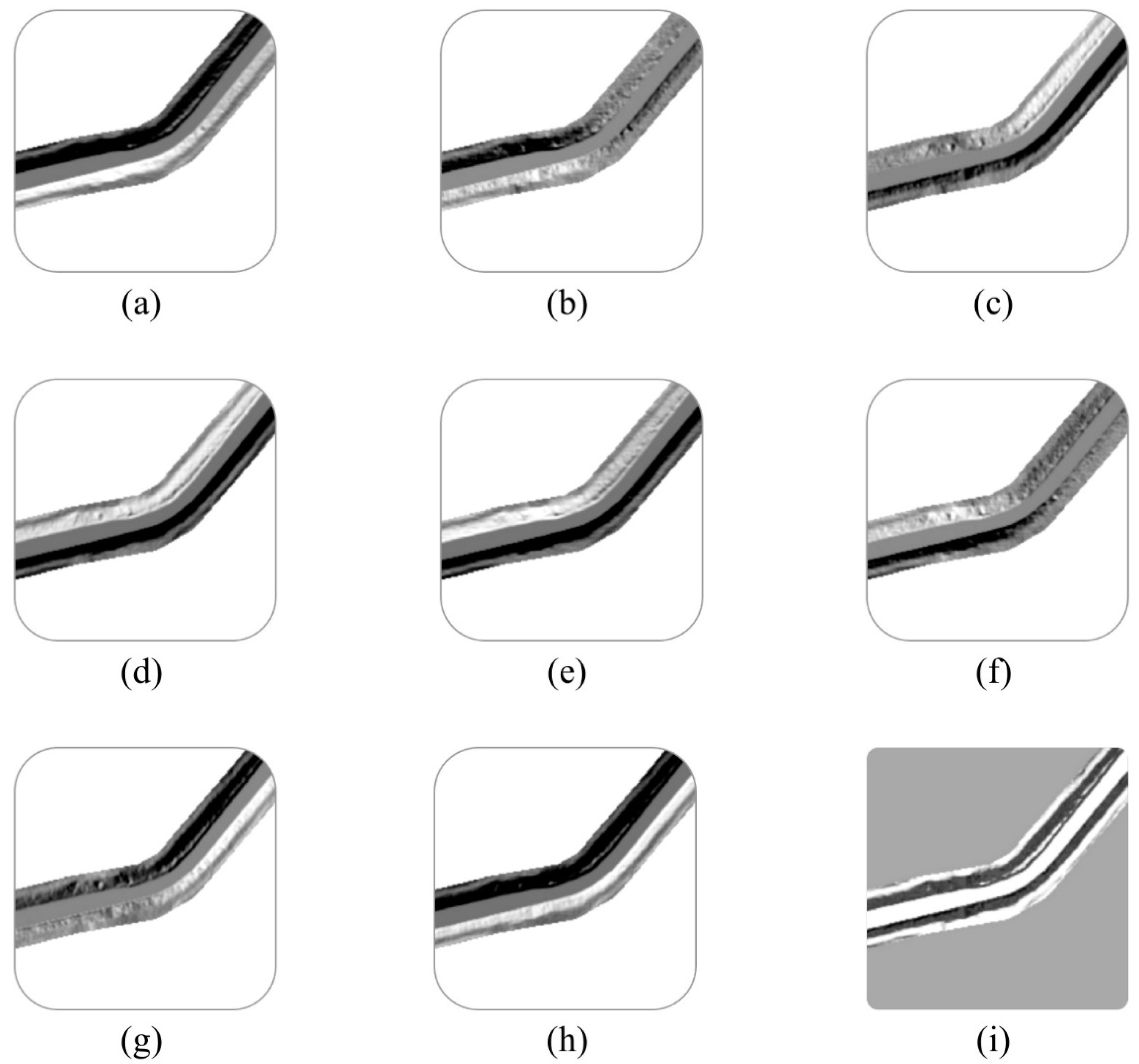
3.1. Hillshade Analysis

Visual inspection of the ditch systems in Waseca County indicates that no system consistently flowed exactly east to west or north to south. Drainage ditches meander through the landscape, typically with a downward slope towards the watershed outlet. Therefore, the eight different azimuth angles that were applied to process the exaggerated DEM helped in addressing the meandering nature of drainage systems. It is clear from Figure 7 that each hillshade raster shaded and illuminated different parts of the landscape based on the azimuth angle. Figure 7i illustrates the combined output of eight rasters (Figure 7a–h) that was obtained simply by adding the cell values together. The cell values (brightness) in the combined hillshade raster ranged from 686 to 860. Those values that are higher represent the areas highly illuminated, while lower values represents the areas with varying degrees of illumination. When the raster was visualized at a small scale, it shows a well-defined drainage ditch berm. However, closer inspection (large scale) reveals a less defined transition between the berm and adjacent relatively flat areas. Interestingly, in the combined raster (Figure 7i) the stream channel also appears as part of the highly illuminated values.

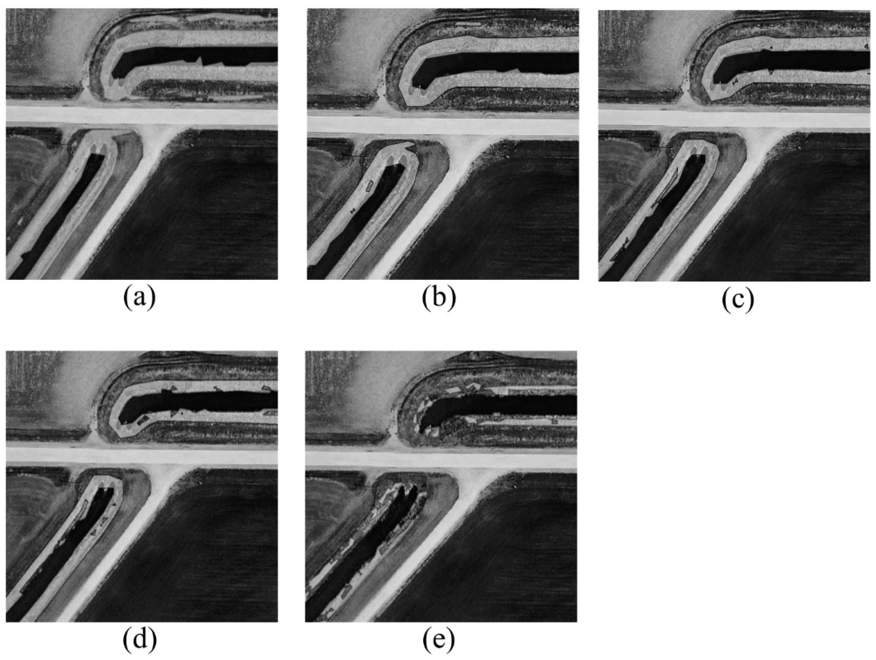
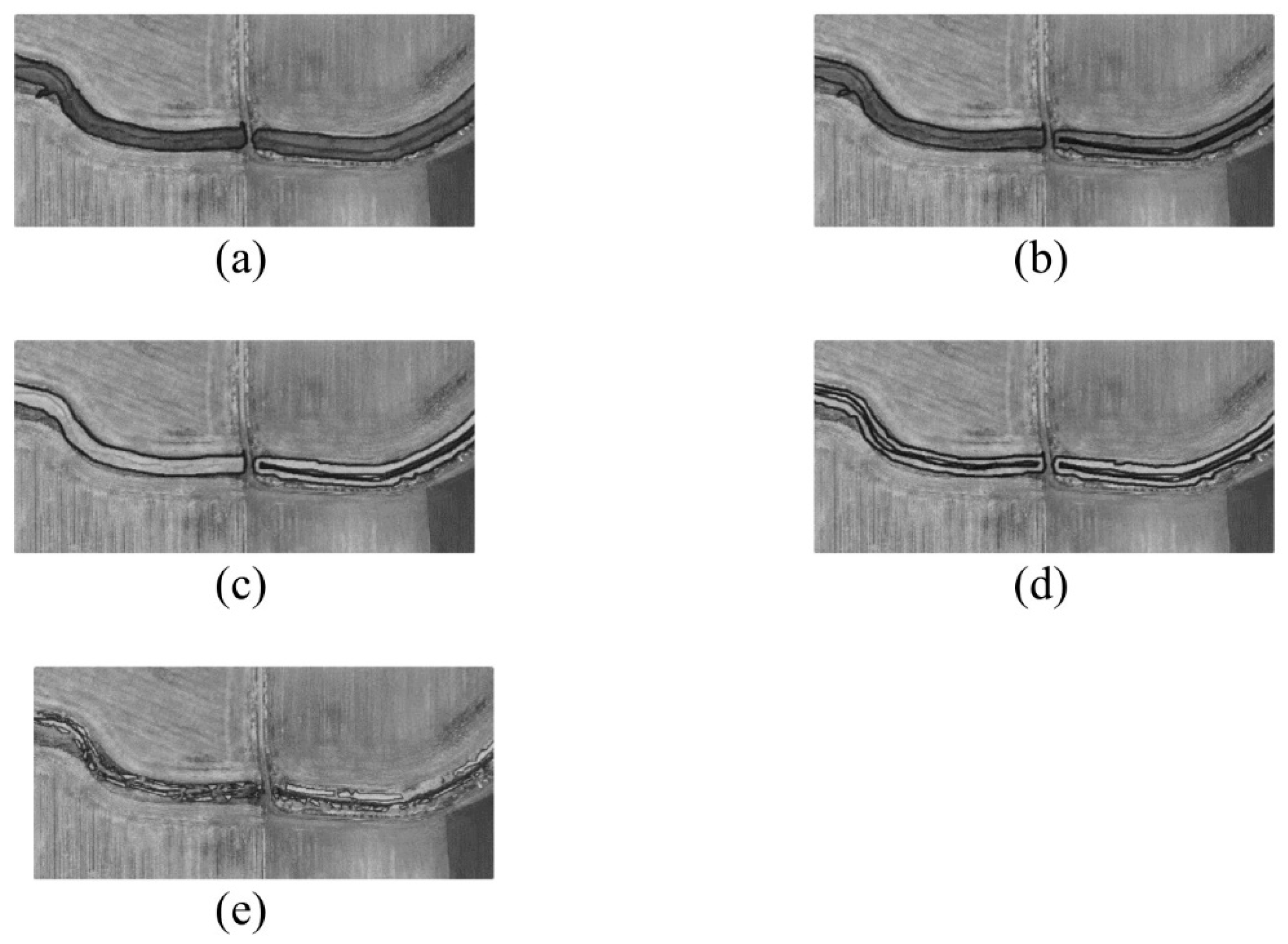
3.2. Berm Extraction

GPS points that were identified as the top of berm in conjunction with the results of the combined hillshade raster helped delineate the transition between landforms. With the help of the normal distribution plot (Figure 5) the mean cell value, the cell values at ±0.5 SD, and the cell values at ±1 SD were extracted (Table 1) and used to identify the top of the berm. Figure 8 shows five berm polygon outputs based on the extracted mean cell value, the cell values at ±0.5 SD, and the cell values at ±1 SD. Figure 8a,b outputs included outlying polygon features that were most likely not berm. These polygon features included other landforms such as roadside ditches and low points in the landscape near the drainage ditch system. The other three results (Figure 8c–e) were less significant with lesser percentages of complete berms. Figure 9 shows the complete berms extracted after the sliver polygons were eliminated and water channels were included through the “Union” tool. The result shows that the polygons extracted for +0.5 SD and +1 SD values resulted in much more complete polygons. These filled-in berm polygons were associated with varying amounts of fragmented polygons and jagged berm edges as seen in Figure 8 and Figure 9. The results produced different percentages of completed berms ranging between 3.20% to 79.80% of the linear length of the ditch system. It was observed that the higher and the lower percentages of the ditch berms are complete, and more manual manipulation was required to remove the jagged berm edges or additional fragmented polygon features identified as berm. The calculated percentages of berm that is considered complete (Table 1) indicates that when the +1 SD cell value was used for berm extraction, the berms were most complete (79.80%) followed by +0.5 SD cell value (67.30%).

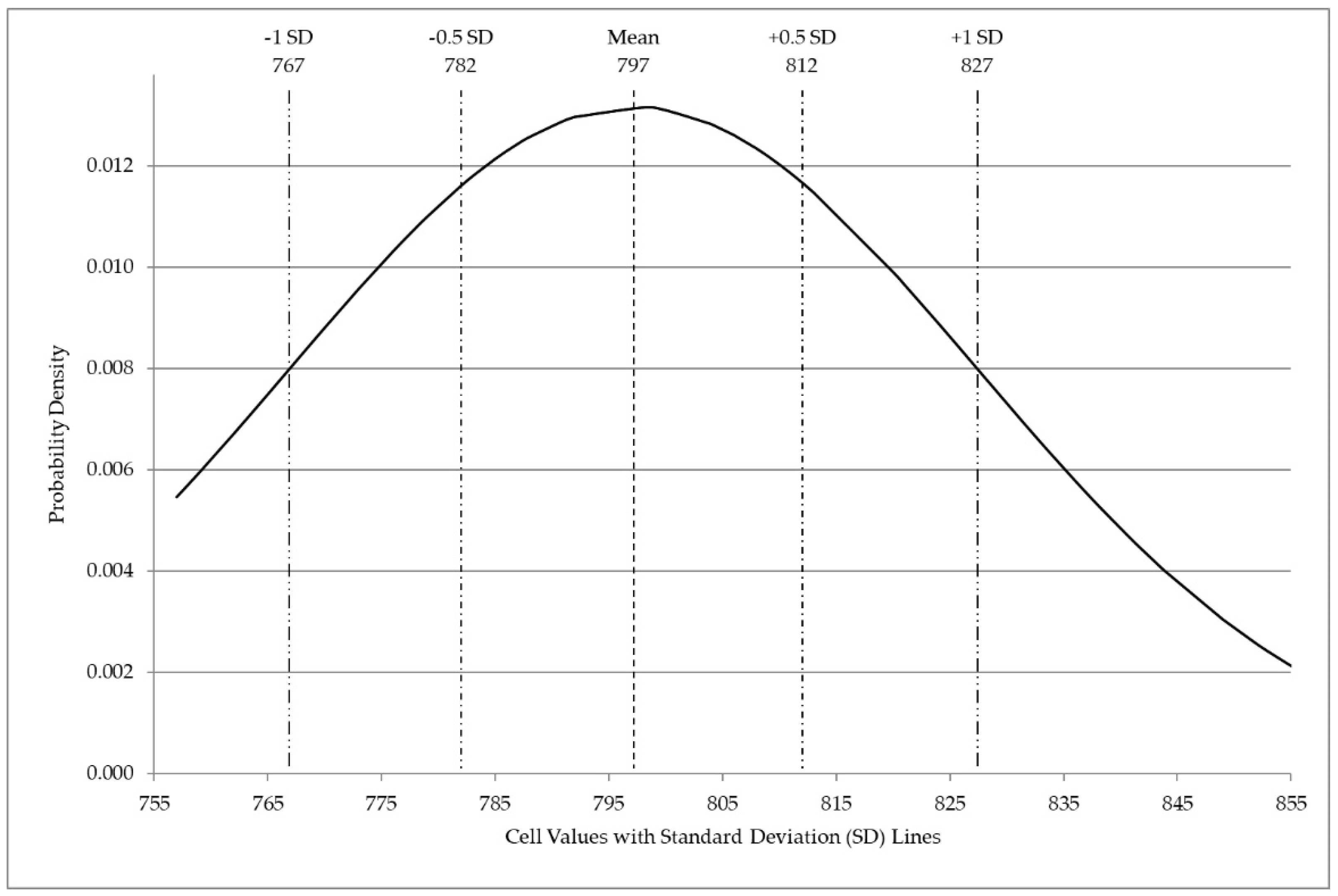
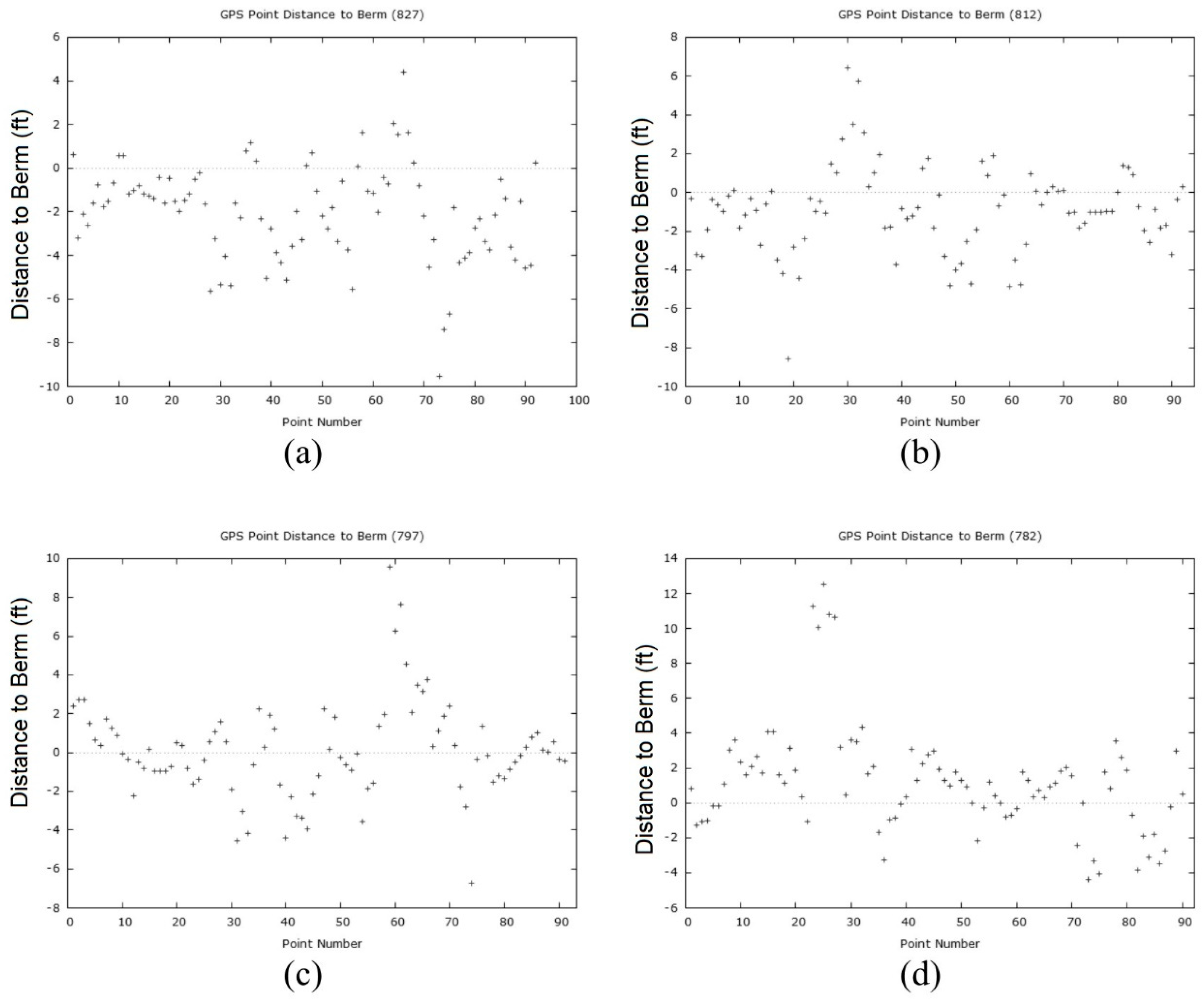
3.3. Accuracy Estimation

Each berm output, except for the −1 SD (cell value 767), were used to validate accuracy by comparing the distance between the top of the berm as noted in the field and the result obtained through geoprocessing. The –1 SD berms were not used for accuracy estimation as it lacked a usable berm edge to identify the linear distance between GPS points collected in the field and modeled berm output. The other four extraction values (mean cell value, the cell values at ±0.5 SD, and the cell value at +1 SD) were used to estimate accuracy of the model outputs. The +1 SD (cell value 827) berm had an average distance of −2.01 ft, which indicates that most of the GPS points were below the berm line. This break value had the range of 13.93 ft between the furthest positive distance (outside the berm) and negative distance (inside the berm). The standard deviation of 2.22 ft indicates that most GPS points were within the cell size of the raster used. The +0.5 SD (cell value 812) berm had an average distance of −0.94 ft, indicating that most of the GPS points were slightly below the berm line. The range increased from 13.93 ft to 15 ft when the cell value 827 and the cell value 812 berms were compared respectively. The standard deviation of 2.25 ft is slightly higher than that of the berm of +1 SD (cell value 827). This indicates that most of the GPS points were closer to the berm line in the case of cell value 812 than the cell value 827. In both these cases, the average distance was within the cell size (3.28 ft) of the raster that was used for modeling. The mean (cell value 797) berm produced the closest results of 0.08 ft average distance to berm line from the GPS points. The range of the distance increased to 16.3 ft, and the standard deviation increased to 2.45 ft. This standard deviation value is still within the cell size of the raster that was used to build the model. Finally, the −0.5 SD (cell value 782) berm was tested for accuracy and returned a 1.22 ft average distance. The range increased to 16.89 ft between the positive and negative values. The standard deviation crept up to 3.12 ft, which is slightly under the cell size of the raster 3.28 ft (1 m). The mean break value (cell value 797) had the closest average distance to berm edges, which was expected. This suggests that the mean and +0.5 SD values (cell value 797 and 812) best represent the values to extract berm edges from the combined hillshade raster. However, upon viewing the results, the +0.5 SD extraction value of 812 appeared to be the best suited.

3.4. Landuse Types within Buffer Area

While assessing the land-use types within the statutory buffer area, during the final modelling phases, the +0.5 SD and +1 SD values were used to prepare the ditch buffers. Although the +0.5 SD seems best suitable for extracting the berm for creating statutory buffer, as +1 SD berm was more complete (79.80%), the study also experimented with that berm. Both these values (+0.5 SD: cell value 812 and +1 SD: cell value 827) were applied to rerun the entire model for the whole Waseca County. After extracting the berms for all the ditch systems within the county, buffers were used to quantify the degree of probable acreage violation within the statutory buffer distance of 16.5 ft. As tillable area is one of the major probable violation land-use types, the difference between the two values (+0.5 SD and +1 SD) were compared, and it was found that there is a 3% difference. Table 2 shows various land-use types as designated by Waseca County that occur within the buffer area of the identified complete berm polygon of +0.5 SD; results are listed in descending order of probable violation acreages within ditch systems (Table 2). Other land-use types in Table 2 are typically allowed within the ditch system buffer areas and are included for comparison purposes.

4. Discussion

4.1. Importance of Results

Extraction of DEM using the 75 ft buffer from the centerline of ditch systems allowed a manageable area to model ditch berm extraction while reducing processing time. It should be noted that 75 ft buffer is not an absolute value and buffer distance can vary based on the study site and computational abilities. A slight exaggeration of 1.5 times was helpful in highlighting minor changes between cell values. In this study, multiple levels of exaggeration such as two, three, and five times were experimented to observe the effect. However, it was found that the cell values that represent elevation when exaggerated greater than 1.5 times were leading to too much of ambiguity while locating the top of the berm. Therefore, for modeling purposes, the study used the 1.5 times exaggerated elevation values. By doing this, the goal of slightly modifying cell values to reflect minor changes and not overemphasize vertical changes was achieved. Using hillshade as the main input data in the modelling technique ensures that landforms that change through the landscape are modelled in a uniform way, without a complicated index calculation that depends on many control variables. In this research, 1 m (3.28 ft) DEMs were used that were the best available data for Waseca County, Minnesota. Further research is required to analyze the effect of higher resolution DEMs on the model outcome; maybe with higher resolution DEMs more accurate results could be produced.
Another requirement for constructing the model was the GPS spot elevation data points. Without identifying the transition points for the berm, the model could not have produced any useful result. One of the major challenges for the research was collecting the GPS data points and identifying points that represents the top of the berm in the field; it was time taking. In this research, around 2000 GPS points were collected from over 96 transect lines. While locating the top of the ditch berms, the identified points in the field were considered more reliable during the review process, and only in three locations the top of ditch berm that was based on the field notes were modified. These modifications were conducted based on the assumed top of the berm line and changes were restricted to the adjoining cell. The established model was useful for both natural drainage ditch systems and areas where humans have engineered drainage ditch systems. User input is still required for some of the model outputs; however, the model drastically reduces editing time for the user while producing relatively accurate results. As the model was not successful in obtaining 100% complete berm polygons for the entire length of the ditch systems and there were fragmented berm polygon features within and nearby, it required manual intervention to identify the edge of the landform and remove those fragmented polygons.
The research successfully used the model derived +0.5 SD and +1 SD values of the combined hillshade raster (cell values of 812 and 827, respectively) to obtain complete berm polygons for the entire Waseca County. These boundary polygons were used to create statutory buffers (16.5 ft) and estimate different land-use acreages within those buffered areas. It was found that tillable area was one of the major probable violation of land-use types within these buffered areas. The findings from such models could give the authorities options to quickly look into existing conditions and decide on a future course of action. In the absence of an easy and simple model available to map these drainage landforms and ditch berms in an accurate and timely manner, the proposed model could be used by many counties in Minnesota and around the world. Incorporating additional information such as topographic position index (TPI) to further refine the model output could be attempted in future research.

4.2. Landscape Planning Modeling and Management

From time immemorial, understanding and altering landscape has long fascinated humanity. Whether it is the identification of formations such as mountains, rivers, hills, cliffs, etc., or designing them to support human need, landscape has played a major role. It is presumed that ancient farmers were possibly aware of the benefits of draining wetlands for agricultural purposes. Drainage, through which waters are removed from the landscape via channelized watercourses, are integral to landscape planning and management. For environmental sustainability, and sustainable agricultural practices, properly designed drainage systems and landscape planning is essential. Principles of landscape design can be further extended to restore drainage systems and understand aquatic ecological integrity [59,60,61,62].
Recognizing the importance of drainage landforms and surrounding landscape public policies are framed all over the world so that landscapes can be properly planned to manage land and water. For example, in Minnesota, USA, there are legal descriptions relating to delineation of drainage landforms so that buffer strips can be placed to help manage land and water in a sustainable manner. These state statutes categorically define how to identify the boundary between ditches and the remaining landscape. Furthermore, there is specific information about the width of the buffer strips to be established on public drainage systems. It is important to note that Minnesota legislators saw fit to define a landform by statute to further reductions in water pollution from agricultural practices. However, there is no method of mass identification for mapping these drainage landforms.
Drainage landforms present a unique challenge in mass automated GIS mapping due to their tendency to meander through the landscape. In this research, the geospatial modeling approach returned useable results for most of the linear length of open drainage ditch systems in Waseca County, Minnesota. The modelling approach accomplished the goal of the research partially. A 100% automated model would have been ideal; however, the model produced by the research automated the output for around 80% of the linear length of ditch systems. The best automated model, with highly dependable parameters could extract complete ditch berm polygons for approximately 68% of the linear length of the ditch systems. It may be improbable to produce a model that will fully automate the identification of the drainage landforms, specifically the drainage ditch berms in the landscape. Problem areas will continue to be areas where drainage systems flatten and appear to be the same with the surrounding landscapes in the DEM data. These results, while not perfect outcomes, are still promising for mapping ditch berms for compliance with state statutes. Therefore, drainage landforms can be identified in the landscape when the appropriate scale and boundary definitions are used. Nonetheless, it requires knowledge of the spatial extent that defines the feature within the landscape.

5. Conclusions

Whether it is natural or engineered, drainage is integral to the landscape through which waters are removed via channelized watercourses. These landforms have recently become important to local and state governments in Minnesota and around the world for the purposes of installing grass buffer strips. Additionally, identifying the top of drainage berms in the landscape has become desirable for environmental stewards and those enforcing drainage laws. This research set out to identify where drainage systems, particularly drainage ditches, transition to the surrounding landscape using an automated geospatial modeling approach. Although the established modeling approach could not delineate 100% complete ditch berms for all the ditches in Waseca County, Minnesota, the result is very promising, as the study could largely identify berm boundaries and create berm polygons that separate the ditches from the surrounding landscape. Using these identified boundaries, statutory ditch buffers measured 1 rod or 16.5 ft from the top of the berm were created. Using these buffer outputs, tillable land-use areas could be identified, which are the only land-use types currently identified as not exempt from buffer rules in the State of Minnesota. As the top of the berm is a gradually changing landscape from berm to other landforms, on the ground, the top of the berm was difficult to identify as well. However, governments that are tasked with enforcing compliance can potentially use this model-derived information to start working with landowners while ensuring compliance. Moreover, this could allow local governments to target their resources for compliance enforcement as compared to sending workers to walk the length of the ditch systems locating the top of berms.

Author Contributions

Conceptualization, J.G., and N.F.; investigation, J.G., R.M., and N.F.; methodology, J.G., and N.F.; data curation, J.G., and N.F.; validation, J.G., and N.F; visualization, J.G.; formal analysis, J.G., and R.M.; writing—original draft, J.G.; writing—review and editing, J.G., and R.M. All authors have read and agreed to the published version of the manuscript.

Funding

This research received no external funding.

Conflicts of Interest

The authors declare no conflict of interest.

References

  1. Minár, J.; Evans, I.S. Elementary forms for land surface segmentation: The theoretical basis of terrain analysis and geomorphological mapping. Geomorphology 2008, 95, 236–259. [Google Scholar] [CrossRef]
  2. Evans, I.S. Geomorphometry and landform mapping: What is a landform? Geomorphology 2012, 137, 94–106. [Google Scholar] [CrossRef]
  3. Strahler, A.N. Quantitative analysis of watershed geomorphology. Trans. Am. Geophys. Union 1957, 38, 913–920. [Google Scholar] [CrossRef] [Green Version]
  4. Wilson, J.P. Digital terrain modeling. Geomorphology 2012, 137, 107–121. [Google Scholar] [CrossRef]
  5. Blaszcynski, J.S. Landform characterization with geographic information systems. Photogramm. Eng. Remote Sens. 1997, 63, 183–191. [Google Scholar]
  6. Bishop, M.P.; James, L.A.; Shroder, J.F.; Walsh, S.J. Geospatial technologies and digital geomorphological mapping: Concepts, issues and research. Geomorphology 2012, 137, 5–26. [Google Scholar] [CrossRef]
  7. Drăguţ, L.; Eisank, C. Object representations at multiple scales from digital elevation models. Geomorphology 2011, 129, 183–189. [Google Scholar] [CrossRef] [Green Version]
  8. Fisher, P.; Wood, J.; Cheng, T. Where is Helvellyn? Fuzziness of multi-scale landscape morphometry. Trans. Inst. Br. Geogr. 2004, 29, 106–128. [Google Scholar] [CrossRef]
  9. Schmidt, J.; Hewitt, A. Fuzzy land element classification from DTMs based on geometry and terrain position. Geoderma 2004, 121, 243–256. [Google Scholar] [CrossRef]
  10. Weissel, J.K.; Pratson, L.F.; Malinverno, A. The length-scaling properties of topography. J. Geophys. Res. Space Phys. 1994, 99, 13997–14012. [Google Scholar] [CrossRef]
  11. Heimlich, R.E.; Wiebe, K.D.; Claassen, R.; Gadsby, D.; House, R.M. Wetlands and Agriculture: Private Interests and Public Benefits; Resource Economics Division, Economic Research Service, US Department of Agriculture: Washington, DC, USA, 1998.
  12. Smedema, L.K.; Vlotman, W.F.; Rycroft, D. Modern Land Drainage: Planning, Design and Management of Agricultural Drainage Systems; CRC Press: Abingdon, UK, 2004. [Google Scholar]
  13. Skaggs, R.W.B.; Brevé, M.A.; Gilliam, J.W. Hydrologic and water quality impacts of agricultural drainage*. Crit. Rev. Environ. Sci. Technol. 1994, 24, 1–32. [Google Scholar] [CrossRef]
  14. Strock, J.S.; Dell, C.J.; Schmidt, J.P. Managing natural processes in drainage ditches for nonpoint source nitrogen control. J. Soil Water Conserv. 2007, 62, 188–196. [Google Scholar]
  15. Montgomery, D.R. Road surface drainage, channel initiation, and slope instability. Water Resour. Res. 1994, 30, 1925–1932. [Google Scholar] [CrossRef]
  16. Dahl, T.E.; Allord, G.J. History of Wetlands in the Conterminous United States; Fretwell, J.D., Williams, J.S., Redman, P.J., Eds.; National Water Summary on Wetland Resources, USGS Water-Supply, Paper US Geological Survey: Washington, DC, USA, 1996; Volume 2425, pp. 19–26.
  17. Pavelis, G.A. Farm Drainage in the United States: History, Status, and Prospects; US Department of Agriculture, Economic Research Service: Washington, DC, USA, 1987.
  18. Tiner, R.W., Jr. Wetlands of the United States: Current Status and Recent Trends; National Wetlands Inventory; Newton Corner, Massachusetts, US Department of the Interior, Fish and Wildlife Service: Washington, DC, USA, 1984. [Google Scholar]
  19. Glaser, P.H.; Wheeler, G.A.; Gorham, E.; Wright, H.E. The Patterned Mires of the Red Lake Peatland, Northern Minnesota: Vegetation, Water Chemistry and Landforms. J. Ecol. 1981, 69, 575–599. [Google Scholar] [CrossRef]
  20. Burwell, R.W.; Sugden, L.G. Potholes—Going, going. In Waterfowl Tomorrow; US Fish and Wildlife Service: Washington, DC, USA, 1964; pp. 369–380. [Google Scholar]
  21. Frayer, W.E. Status and Trends of Wetlands and Deepwater Habitats in the Conterminous United States, 1950’s to 1970’s; Dept. of Forest and Wood Sciences, Colorado State University: Fort Collins, CO, USA, 1983. [Google Scholar]
  22. Claassen, R.; Cattaneo, A.; Johansson, R. Cost-effective design of agri-environmental payment programs: U.S. experience in theory and practice. Ecol. Econ. 2008, 65, 737–752. [Google Scholar] [CrossRef]
  23. Ribaudo, M.; Hoag, D.L.; Smith, M.E.; Heimlich, R. Environmental indices and the politics of the Conservation Reserve Program. Ecol. Indic. 2001, 1, 11–20. [Google Scholar] [CrossRef]
  24. Stuart, D.; Gillon, S. Scaling up to address new challenges to conservation on US farmland. Land Use Policy 2013, 31, 223–236. [Google Scholar] [CrossRef]
  25. Gene, S.; Hoekstra, P.; Hannam, C.; White, M.; Truman, C.; Hanson, M.; Prosser, R. The role of vegetated buffers in agriculture and their regulation across Canada and the United States. J. Environ. Manag. 2019, 243, 12–21. [Google Scholar] [CrossRef]
  26. Kreig, J.A.; Ssegane, H.; Chaubey, I.; Negri, M.C.; Jager, H.I. Designing bioenergy landscapes to protect water quality. Biomass Bioenergy 2019, 128, 10532. [Google Scholar] [CrossRef]
  27. Srinivas, R.; Drewitz, M.; Magner, J. Evaluating watershed-based optimized decision support framework for conservation practice placement in Plum Creek Minnesota. J. Hydrol. 2020, 583, 124573. [Google Scholar] [CrossRef]
  28. Planting Ditches with Perennial Vegetation, Minnesota Statutes 2019. Available online: https://www.revisor.mn.gov/statutes/cite/103E.021 (accessed on 5 November 2020).
  29. Riparian Protection and Water Quality Practices, Minnesota Statutes 2019. Available online: https://www.revisor.mn.gov/statutes/cite/103F.48 (accessed on 5 November 2020).
  30. Miller, T.P.; Peterson, J.R.; Lenhart, C.F.; Nomura, Y. The Agricultural BMP Handbook for Minnesota; Minnesota Department of Agriculture: St. Paul, MN, USA, 2012.
  31. Xu, S.; Li, S.-L.; Zhong, J.; Li, C. Spatial scale effects of the variable relationships between landscape pattern and water quality: Example from an agricultural karst river basin, Southwestern China. Agric. Ecosyst. Environ. 2020, 300, 106999. [Google Scholar] [CrossRef]
  32. Mayer, P.M.; Reynolds, S.K., Jr.; McCutchen, M.D.; Canfield, T.J. Meta-Analysis of Nitrogen Removal in Riparian Buffers. J. Environ. Qual. 2007, 36, 1172–1180. [Google Scholar] [CrossRef] [PubMed]
  33. Yamada, T.; Logsdon, S.D.; Tomer, M.D.; Burkart, M.R. Groundwater nitrate following installation of a vegetated riparian buffer. Sci. Total. Environ. 2007, 385, 297–309. [Google Scholar] [CrossRef] [PubMed]
  34. Ranjan, P.; Singh, A.S.; Tomer, M.D.; Lewandowski, A.M.; Prokopy, L.S. Lessons learned from using a decision-support tool for precision placement of conservation practices in six agricultural watersheds in the US midwest. J. Environ. Manag. 2019, 239, 57–65. [Google Scholar] [CrossRef] [PubMed]
  35. Devereux, B.J.; Amable, G.; Crow, P.; Cliff, A. The potential of airborne lidar for detection of archaeological features under woodland canopies. Antiquity 2005, 79, 648–660. [Google Scholar] [CrossRef]
  36. An Evaluation of Automated GIS Tools for Delineating Karst Sinkholes and Closed Depressions from 1-Meter LiDAR-Derived Digital Elevation Data. Available online: https://pubs.er.usgs.gov/publication/70195369 (accessed on 5 November 2020).
  37. MacMillan, R.A.; Martin, T.C.; Earle, T.J.; McNabb, D.H. Automated analysis and classification of landforms using high-resolution digital elevation data: Applications and issues. Can. J. Remote. Sens. 2003, 29, 592–606. [Google Scholar] [CrossRef]
  38. McCoy, M.; Asner, G.P.; Graves, M.W. Airborne lidar survey of irrigated agricultural landscapes: An application of the slope contrast method. J. Archaeol. Sci. 2011, 38, 2141–2154. [Google Scholar] [CrossRef]
  39. Doneus, M.; Kühteiber, T. Airborne laser scanning and archaeological interpretation–bringing back the people. In Interpreting Archaeological Topography: Airborne Laser Scanning, 3D Data, and Ground Observation; Occasional Publication of the Aerial Archaeology Research Group, Oxbow Books: Oxford, UK, 2013; pp. 32–50. [Google Scholar]
  40. Lindsay, J.B.; Dhun, K. Modelling surface drainage patterns in altered landscapes using LiDAR. Int. J. Geogr. Inf. Sci. 2015, 29, 397–411. [Google Scholar] [CrossRef]
  41. Magesh, N.S.; Ch, N. A GIS based automated extraction tool for the analysis of basin morphometry. Bonfring Int. J. Ind. Eng. Manag. Sci. Spec. Issue Geospat. Technol. Dev. Nat. Resour. Disaster Manag. 2012, 2, 32–35. [Google Scholar]
  42. Reddy, G.P.O.; Maji, A.K.; Gajbhiye, K.S. Drainage morphometry and its influence on landform characteristics in a basaltic terrain, Central India–a remote sensing and GIS approach. Int. J. Appl. Earth Obs. Geoinf. 2004, 6, 1–16. [Google Scholar] [CrossRef]
  43. Saadat, H.; Bonnell, R.; Sharifi, F.; Mehuys, G.; Namdar, M.; Ale-Ebrahim, S. Landform classification from a digital elevation model and satellite imagery. Geomorphology 2008, 100, 453–464. [Google Scholar] [CrossRef]
  44. Garcia, G.P.; Grohmann, C.H. DEM-based geomorphological mapping and landforms characterization of a tropical karst environment in southeastern Brazil. J. S. Am. Earth Sci. 2019, 93, 14–22. [Google Scholar] [CrossRef] [Green Version]
  45. Jaballah, M.; Camenen, B.; Paquier, A.; Jodeau, M. An optimized use of limited ground based topographic data for river applications. Int. J. Sediment Res. 2019, 34, 216–225. [Google Scholar] [CrossRef]
  46. Prufer, K.M.; Thompson, A.E.; Kennett, D.J. Evaluating airborne LiDAR for detecting settlements and modified landscapes in disturbed tropical environments at Uxbenká, Belize. J. Archaeol. Sci. 2015, 57, 1–13. [Google Scholar] [CrossRef]
  47. Garrison, T.G.; Garrison, T.G.; Firpi, O.A. Recentering the rural: Lidar and articulated landscapes among the Maya. J. Anthr. Archaeol. 2019, 53, 133–146. [Google Scholar] [CrossRef]
  48. Anemone, R.L.; Conroy, G.C.; Emerson, C.W. GIS and paleoanthropology: Incorporating new approaches from the geospatial sciences in the analysis of primate and human evolution. Am. J. Phys. Anthr. 2011, 146, 19–46. [Google Scholar] [CrossRef] [Green Version]
  49. Davis, O. Processing and Working with LiDAR Data in ArcGIS: A Practical Guide for Archaeologists; Royal Commission of the Ancient and Historical Monuments of Wales: Aberystwyth, UK, 2012.
  50. Harmon, J.M.; Leone, M.P.; Prince, S.D.; Snyder, M. Lidar for archaeological landscape analysis: A case study of two eighteenth-century Maryland plantation sites. Am. Antiq. 2006, 71, 649–670. [Google Scholar] [CrossRef]
  51. Verhagen, P.; Drăguţ, L. Object-based landform delineation and classification from DEMs for archaeological predictive mapping. J. Archaeol. Sci. 2012, 39, 698–703. [Google Scholar] [CrossRef]
  52. Chalkias, C.; Faka, A. Risk evaluation by modelling exposure to direct sunlight on rural highways—A GIS approach. In Proceedings of the 11th WSEAS International Conference on Mathematical Methods and Computational Techniques in Electrical Engineering, Athens, Greece, 28–30 September 2009; World Scientific and Engineering Academy and Society (WSEAS): Athens, Greece, 2009; pp. 373–378. [Google Scholar]
  53. Veronesi, F.; Hurni, L. A GIS tool to increase the visual quality of relief shading by automatically changing the light direction. Comput. Geosci. 2015, 74, 121–127. [Google Scholar] [CrossRef]
  54. U.S Census Bureau. 2019, Population Estimates Program. US/PST045219. Available online: https://www.census.gov/quickfacts/fact/table/wasecacountyminnesota (accessed on 5 November 2020).
  55. Minnesota Geospatial Commons. Available online: https://www.mngeo.state.mn.us/chouse/elevation/lidar.html (accessed on 5 July 2019).
  56. ESRI. Hillshade Function. 2020. Available online: https://desktop.arcgis.com/en/arcmap/10.5/manage-data/raster-and-images/hillshade-function.htm (accessed on 5 November 2020).
  57. ESRI. How Filter Works. 2020. Available online: https://desktop.arcgis.com/en/arcmap/10.5/tools/spatial-analyst-toolbox/how-filter-works.htm (accessed on 5 November 2020).
  58. Cottrell, A.; Lucchetti, R. Gretl user ManualGretl user Manual. 2007. Available online: http://gretl.sourceforge.net/ (accessed on 5 November 2020).
  59. Shaker, R.R.; Yakubov, A.D.; Nick, S.M.; Vennie-Vollrath, E.; Ehlinger, T.J.; Forsythe, K. Predicting aquatic invasion in Adirondack lakes: A spatial analysis of lake and landscape characteristics. Ecosphere 2017, 8, e01723. [Google Scholar] [CrossRef] [Green Version]
  60. The Development and Evaluation of Methods for Quantifying Risk to Fish in Warm-water Streams of Wisconsin Using Self Organized Maps: Influences of Watershed and Habitat Stressors. Available online: https://repository.library.northeastern.edu/files/neu:329785 (accessed on 17 November 2020).
  61. Agricultural Land Fragmentation and Biological Integrity: The impacts of a Rapidly Changing Landscape on Streams in Southeastern Wisconsi. Available online: https://static1.squarespace.com/static/5e1253990612347a7d3eb094/t/5e4de32d50bc066ba3f6564f/1582162735857/Shaker_Ehlinger_2007_Aglands_Aquatic_Ecology.pdf (accessed on 17 November 2020).
  62. Todeschini, S.; Papiri, S.; Sconfietti, R. Impact assessment of urban wet-weather sewer discharges on the Vernavola River (Northern Italy). Civ. Eng. Environ. Syst. 2011, 28, 209–229. [Google Scholar] [CrossRef]
Figure 1. Location of ditch systems (JD 11, CD 45, CD 27, JC 6, and CD 48) and GPS data collection sites in Waseca County, Minnesota (44°01′ N, 93°35′ W).
Sustainability 12 09600 g001
Figure 2. GPS transect lines along JD 11: (a) Transect site overview, (b) transect line grouping.
Sustainability 12 09600 g002
Figure 3. Comparison of hillshade rasters using different azimuths: (a) 315°, (b) 90°.
Sustainability 12 09600 g003
Figure 4. Comparison between transect line GPS points and Light Detection and Ranging (LiDAR) digital elevation model (DEM) elevation profiles: (a) Transect line (WGS 1984), (b) LiDAR DEM (UTM Zone 15N). The white point represents the identified top of berm transition point.
Sustainability 12 09600 g004
Figure 5. Normal distribution curve of combined hillshade raster cell values at the field identified top of berm locations.
Sustainability 12 09600 g005
Figure 6. Linear foot distance between GPS points noted as berm in the field to the model delineated top of berm line. (a) Hillshade of cell value 827, (b) hillshade of cell value 812, (c) hillshade of cell value 797, (d) hillshade of cell value 782.
Sustainability 12 09600 g006
Figure 7. Hillshade outputs by azimuth at 25° illumination angle. (a) 0°, (b) 45°, (c) 90°, (d) 135°, (e) 180°, (f) 225°, (g) 270°, (h) 315°, (i) combined raster output.
Sustainability 12 09600 g007
Figure 8. Berm modeling from combined hillshade raster: (a) +1 SD (cell value 827), (b) +0.5 SD (cell value 812) (c) mean (cell value 797) (d) −0.5 SD (cell value 782), (e) −1 SD (cell value 767).
Sustainability 12 09600 g008
Figure 9. Completed berm output, (a) +1 SD (cell value 827) (b) +0.5 SD (cell value 812) (c) mean (cell value 797) (d) −0.5 SD (cell value 782), (e) −1 SD (cell value 7676).
Sustainability 12 09600 g009
Table 1. Modeled berm completion by break value with completion percentage.
STDEVExtracted Cell Value% of Length of Ditch Berms Completed
+182779.80%
+0.581267.30%
Mean79751.70%
−0.578238.70%
−17673.20%
Table 2. Land-use by ditch system within 16.5 ft buffer of +0.5 SD berm.
Ditch SystemTotal Buffer AcresBuilding SiteGrassesLake or WetlandMeadowRight-of-WayWoodTillableViolation Acres
JC 623.111%37%4%0%7%0%51%11.90
JD 5125.482%48%0%0%5%0%46%11.68
CD 8A39.870%25%0%45%3%0%26%10.33
CD 3817.622%22%2%20%3%0%51%9.07
CD 121.841%60%0%5%5%1%28%6.04
CD 357.003%22%0%0%2%0%72%5.03
JD 522.080%67%2%8%1%1%21%4.66
JD 1015.610%47%0%23%1%0%28%4.38
CD 489.780%53%0%0%3%0%43%4.23
CD 475.330%13%0%6%4%0%76%4.07
CD 332.550%30%56%2%1%1%10%3.28
CD 4515.300%65%1%5%6%0%21%3.25
CD 369.731%59%14%0%1%0%25%2.47
CD 3015.410%60%11%6%1%5%16%2.44
CD 504.121%45%0%0%1%0%53%2.19
CD 275.972%37%0%0%15%11%34%2.01
CD 3111.360%42%31%4%6%0%18%2.01
JD 1128.010%84%1%3%4%0%7%1.95
CD 2914.860%50%24%6%7%0%12%1.80
CD 408.800%0%0%63%22%2%12%1.09
CD 262.100%43%0%2%2%2%52%1.08
JD 19.770%94%0%0%0%0%6%0.62
JD 2427.911%82%6%8%1%0%2%0.58
CD 436.000%50%0%16%6%23%4%0.23
JD 84.340%95%0%0%2%0%3%0.12
CD 333.991%81%0%13%2%0%2%0.10
CD 463.000%96%0%0%1%0%2%0.07
CD 15-24.420%98%0%0%0%0%2%0.07
CD 340.350%0%0%50%0%47%3%0.01
CD 281.100%0%52%48%0%0%0%0.00
CD 443.960%12%85%1%3%0%0%0.00
Publisher’s Note: MDPI stays neutral with regard to jurisdictional claims in published maps and institutional affiliations.

