An Overview of Environmental Policies for Mitigation and Adaptation to Climate Change and Application of Multilevel Regression Analysis to Investigate the CO₂ Emissions over the Years of 1970 to 2018 in All Brazilian States

Abstract

Background: Brazil, one of the largest greenhouse gas emitting countries in the world, emitted approximately 2 billion gigatonnes of carbon dioxide (CO₂) in 2018. This data is practically the same recorded in the previous year, suggesting that the country’s trajectory of CO₂ emissions is stabilized. Methods: This study presents an overview of environmental protection and climate change mitigation policies adopted in Brazil, as well as makes use the multilevel regression modeling technique to investigate the relationship between economic activities variables in relation to CO₂ emissions over the years of 1970 to 2018 in all Brazilian states. Results: The results show that the CO₂ emissions in the states have the same behavior as the timeline of the change in land use. Conclusions: The public policies and actions by society and the private sector were fundamental to the reduction verified from the year of 2004 that followed until 2010, both in CO₂ emissions and in the change in land use and forests. As of this year, there has been a trend towards stability in CO₂ emissions. Another important characteristic is that even with a drop in the number of deforestation, the production variables continued to grow, which shows that there may be an increase in production activities, while there is a reduction in deforestation and in CO₂ emissions.

1. Introduction

The United Nations Framework Convention on Climate Change—Paris Agreement is a global commitment approved in 2015 by 195 countries to reduce greenhouse gas emissions, in order to keep the average earth temperature below 2 °C above pre-industrial revolution levels until the end of the century, and to promote efforts so that this warming does not exceed 1.5 °C [1]. Countries agreed to reduce emissions of carbon dioxide (CO₂) and other greenhouse gases (GHG) in the context of sustainable development, and to improve their capability to adapt to the impacts of climate change [1].

Climate change is one of the main challenges facing humanity today, with important consequences for the environment, the society, the economy and the public policies. These challenges represent an opportunity for countries to rethink their strategies for the future and to conduct their actions in accordance with the pillars of sustainable development.

Brazil has taken the lead in global environmental negotiations and the implementation of climate policies in South America, being among the seven largest GHG emitters [2,3] and being the ninth largest economy in the world in terms of nominal GDP [4].

According to data from the Greenhouse Gas Emissions and Removal Estimation System (SEEG), Brazil emitted in 2018 approximately 2 billion tons of carbon dioxide (CO₂) [3,5], representing 1.3% of all GHG greenhouse gas emissions in the world [6].

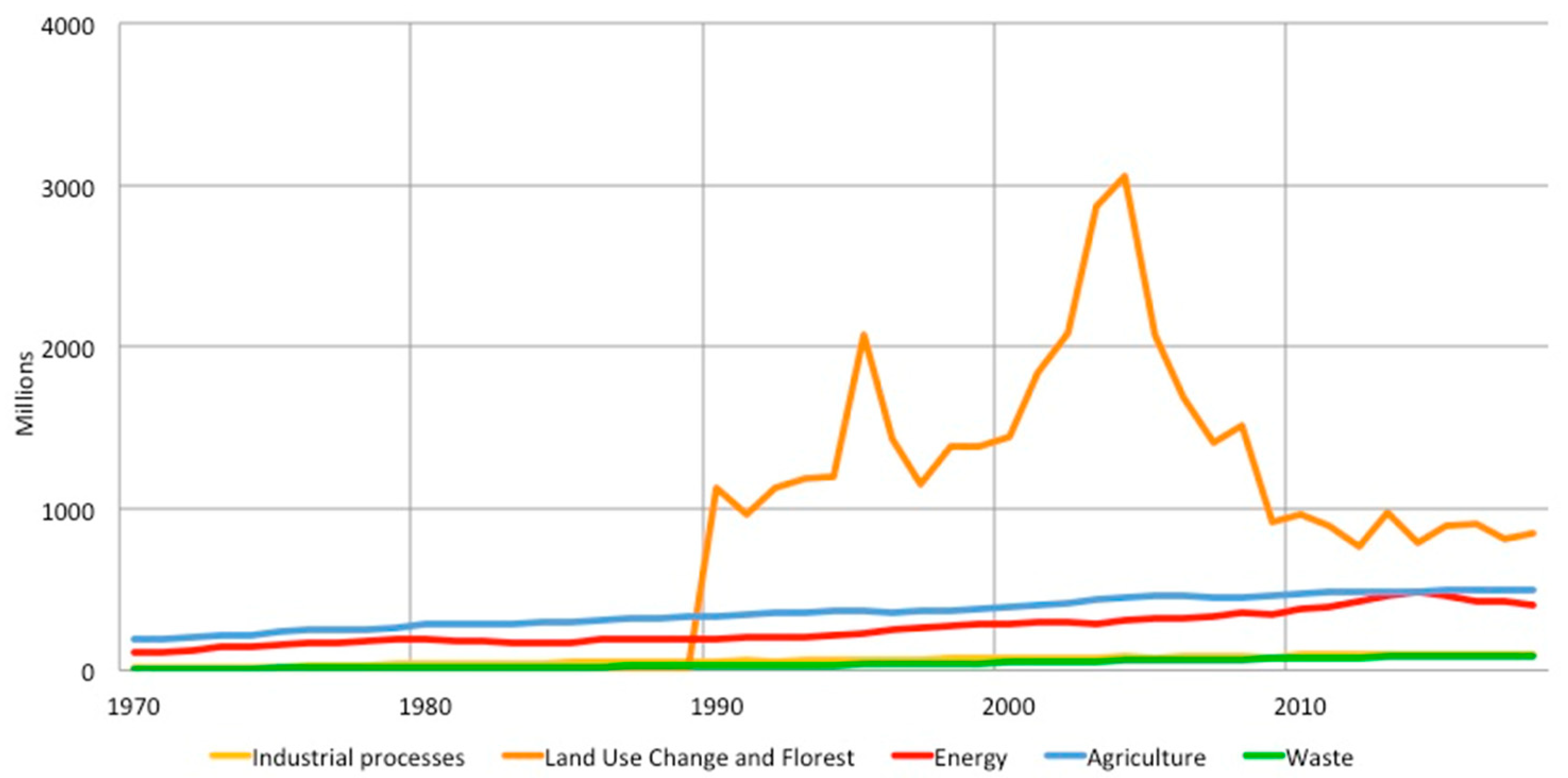
The sector that emits the most GHG is land use change with 46% (845 Mt CO₂), followed by agricultural activities with 24% of emissions and 21% by the energy sector. These data show that although Brazil is an industrialized country, its main emissions do not come from the use of energy that includes all activities that use fossil fuels (407 Mt CO₂), but from the change in land use with the deforestation of forests and agricultural activities [5].

According to Miranda, Brazil has 7.6% of its territory occupied by agricultural activities, being one of the five largest agricultural producers in the world [7]. Data from the Brazilian Agricultural Research Corporation (EMBRAPA) point out that this production would be enough to feed 1 billion people [8]. As agriculture is a climate-dependent activity, studies indicate that climate change could modify global agricultural production and productivity, including Brazilian’s production, putting growth expectations at risk.

In this context, what has Brazil been doing to prevent and or mitigate climate change?

To answer this question, this research presents some government initiatives that were adopted to encourage the development of the sectors, the most relevant being the National Policy on Climate Change (PNMC), the National Plan for Adaptation to Climate Change (PNA), the Sectorial Plan for Mitigation and Adaptation to Climate Change for the Consolidation of a Low Carbon Economy in Agriculture.

Thus, this study intended: (1) to describe the policies for mitigation and adaptation to climate change adopted in the country; (2) to investigate the relation between the variables economic activities and the CO₂ emissions over the years 1970 to 2018 in all Brazilian states using multilevel regression modeling.

Section 2 discusses public policies adopted to prevent and or mitigate climate change in the country. Section 3 details the data collected and the proposed analysis method. Section 4 analyzes the parameters obtained through the multilevel regression model and discusses their empirical and scientific relations. Finally, Section 5 concludes the research.

2. Environmental Protection and Climate Change Policy Structure in Brazil

2.1. National Policy on Climate Change (PNMC)

The National Policy on Climate Change (in Portuguese, Política Nacional sobre Mudança do Clima, PNMC) instituted in Brazil through Law No. 12.187/2009 is one of the main guidelines and instruments for environmental protection and mitigation of climate change, with the objective of reduce its emissions of greenhouse gases (GHG) between 36.1% and 38.9% in relation to projected emissions until 2020 [9]. To accompany the fulfillment of the national commitment to reduce emissions, the PNMC was structured in four main axes: (i) mitigation opportunities, (ii) impacts, vulnerabilities and adaptation, (iii) research and development, and (iv) education, training and communication.

The PNMC provides differentiated actions for each axis, defines mitigation with a focus on forests, agricultural systems, energy, waste, construction, industry and transport, with technological changes and substitutions that reduce the use of resources and emissions per unit of production, as well as the implementation of measures that reduce GHG emissions and increase sinks. In addition, it defines impact with a focus on human and natural systems where everyone has a duty to act, for the benefit of present and future generations, to reduce climate impacts. It also defines adaptation with a focus on health, agricultural systems, water resources, coastal and marine areas, and natural ecosystems with initiatives and measures to reduce the vulnerability of natural and human systems to the current and expected effects of climate change [9].

According to Di Gregorio et al. 2016 [10], agricultural areas, coastal areas, natural ecosystems and water resources are the places where political integration between mitigation and adaptation are the most likely to be achieved and the deforestation of forests is considered especially for their mitigation potential.

Brazilian GHG emissions come mainly from the activities of land use change and forest, agriculture, energy, industrial processes and waste, as shown in Figure 1.

Brazilian GHG emissions differ from emissions from other countries mainly due to the deforestation of forests, which is an important emission factor. Thus, the efforts and guidelines of the PNMC are also in relation to controlling deforestation.

Through the PNMC, Decree No. 9.578 prepared action plans for preventing and controlling deforestation in biomes and sectoral plans for mitigating and adapting to climate change, namely: (I) Action Plan for the Prevention and Control of Deforestation in the Legal Amazon (PPCDAm); (II) Action Plan for the Prevention and Control of Deforestation and Burning in the Cerrado (PPCerrado); (III) Decennial Plan for the Expansion of Energy (PDE); and (IV) Sectorial Plan for Mitigation and Adaptation to Climate Change for the Consolidation of a Low Carbon Economy in Agriculture (ABC Plan) [11].

The data in Figure 1 draw attention to the sector of land use change and forests and the participation of the agricultural sector in GHG emissions and their mitigation potential. Note that GHG emissions from the sector of change and use of land and forests grew in the period 1990 to 2004, driven by deforestation of the Amazon and Cerrado. Over three phases of implementation (2004 to 2008, 2009 to 2011, and 2012 to 2015), the PPCDAm and PPCerrado have contributed to a reduction in the deforestation rate in the Amazon and Cerrado, where the first phase (2004 to 2008) provided the most significant results, contributing to the mitigation of GHG emissions. The PPCDAm and PPCerrado were integrated into the instrument of the National Plan on Climate Change [11].

2.2. National Plan for Adaptation to Climate Change (PNA)

As a result of the PNMC, the Executive Group of the Interministerial Committee on Climate Change (GEx-CIM) developed the National Plan for Adaptation to Climate Change (PNA), which aims to propose initiatives for the management and reduction of climate risk over the long term [12]. The PNA was established by Ordinance No. 150, of the Ministry of the Environment in 2016, as a government effort in partnership with society and the private sector, aiming to implement the National Policy on Climate Change and contribute to the achievement of commitments assumed within the scope of Brazil’s Nationally Determined Contribution to the Paris Agreement (NDC) [13]. The NDC gives the PNA the role of promoting the resilience of ecosystems, infrastructure and production systems. In a debate between society, governments and the private sector, the following objectives were defined for the PNA. Objective 1 concerns the expansion and dissemination of scientific, technical and traditional knowledge: production, management and dissemination of information about risk climatic; Objective 2 deals with coordination and cooperation between public bodies and society.

According to Ministry of the Environment [14], the following actions stand out as being carried out within the scope of Objective 1: the mapping at a municipal scale of Brazil’s vulnerability to droughts; the structuring and development of the adaptation knowledge platform; the mapping of the biophysical impacts of climate change in the Atlantic Forest; and the generation of the Municipal Vulnerability Index to Climate Change, for 6 Brazilian states (Espírito Santo, Pernambuco, Paraná, Maranhão, Amazonas and Mato Grosso do Sul), through the implementation of the Climate Vulnerability System Project (SISVUCLIMA). For Objective 2, actions aimed at expanding coordination between public policies to reduce climate risk in the country stand out, with emphasis on the implementation of the National Policy for Civil Protection and Defense, the National Water Resources Policy and the National Policy National Urban Mobility Program.

2.3. Sectorial Plan for Mitigation and Adaptation to Climate Change for the Consolidation of a Low Carbon Economy in Agriculture (ABC PLAN)

Following the guidelines of the PNMC in Article 11, the Executive Branch established the sectorial Plan for mitigating and adapting to climate change, encouraging the development of sustainable practices in agriculture that reduce anthropogenic GHG emissions and increase carbon sequestration, as well as in other sectors of the economy [9,15]. The ABC Plan created in 2012 is a public policy that presents actions to encourage and monitor the adoption of good practices that prevent deforestation, that reduce emissions and generate resistance to production systems, without compromising productivity and growth in the sector, with execution deadline until the end of 2020.

The agricultural sector is undoubtedly one of the most affected by climate change. Long periods of drought, heavy rain, high temperatures, pests and diseases can damage production, livestock and destabilize the food supply [5]. Seven programs were incorporated into the ABC Plan, six related to mitigation technologies and one with actions to adapt to climate change: they are the Recovery of Degraded Pastures, Adoption of the Crop-Livestock-Forest Integration System (ICLF) and Agroforestry Systems; the Expansion of the No-Tillage System (NTS); the expansion of the use of Biological Nitrogen Fixation (BNF); Increased Area of Planted Forests; Animal Waste Treatment; and Adaptation to Climate Change.

In each program, several actions were taken. In the program for adaptation to climate change, the strategy adopted is to invest more effectively in agriculture, promoting diversified systems and the sustainable use of biodiversity and water resources, with support for the transition process, organization of production, guarantee of income generation, research with genetic resources and breeding, water resources, adaptation of productive systems, identification of vulnerabilities and modeling, among other initiatives [15]. In the program for Planted Forests, the strategy is to promote reforestation actions in the country, expanding the reforested area destined to the production of fibers, wood and cellulose, contributing to the capture of CO₂.

According to Ministry of Agriculture [16], the ABC Plan achieved advances eliminating in the period from 2010 to 2018 between 100.21 and 154.38 million MG CO₂. Several scientific researches have been conducted with the objective of investigating the ABC Plan. FERNANDES, Milton Marques et al. (2020) described the dynamics of land use and occupation in the semiarid region of the state of Sergipe, Brazil, between 1992 and 2017, and simulated land use and occupation for 2030 [17]. Rodrigues, W., and Melo, J. A. (2017) provided in the work “Economic Evaluation of Low Carbon Agriculture Technologies in Savanah Regions” an overview of Brazil’s actions in relation to the agricultural sector, providing a critical analysis of how these actions are being implemented [18]. TERRA, Ana Beatriz C. et al. (2019) presented techniques for recovering degraded pastures involving the use of forage legumes and the association with nitrogen-fixing bacteria in order to increase pasture productivity, making the system sustainable [19].

Although much research has been carried out with important results, the current chief executive of Brazil in his first environmental measure, changed the structure of the Ministry of the Environment [14], handing over forest management to the Ministry of Agriculture (MA) and extinguished the Secretariat of Climate Change and Forests that was responsible for coordinating the implementation of emission reduction policies of the National Plan for Adaptation to Climate Change, and the plans for prevention and control of deforestation in the Amazon (PPCDAm) and Cerrado (PPCerrado). With the shift in emphasis from MMA to MA and the extinction of the Secretary of Climate Change and Forests, the policies and their action plans are undefined [20].

3. Material and Methods

This section describes the main policies for the prevention and mitigation of climate change adopted in Brazil. It investigates the relationship of the variable economic activities in relation to the emissions of carbon dioxide (CO₂) of the global warming potential (GWP) according to the conversion factors established in the 5th report of Intergovernmental Panel on Climate Change (IPCC) AR5 from 1970 to 2018 (last year with available data) for all Brazilian states. The database used was prepared by the Ministry of Science, Technology and Innovation (MCTI), with data obtained from government reports, institutes, research centers, sectoral entities and non-governmental organizations, and is available on the Emissions Estimation System page and Removal of Greenhouse Gases (SEEG) promoted by the Climate Observatory (OC). The different variables of economic activities analyzed are defined in

Table 1. Economic activity variables analyzed.

Initials	Variable	Initials	Variable
TCSNF	Total consumption of synthetic nitrogen fertilizer	TLUC	Total land use and change
SP	Sugar Production	AAP	Adipic acid production
AP	Alcohol Production	StP	Steel production
ScP	Sugarcane Production	AlP	Aluminum production
BP	Beef Production	CeP	Cement Production
MP	Milk Production	ONGP	Oil and natural gas production
CP	Corn Production	HES	Hydrous Ethanol Sales
SoyP	Soy Production	GS	Gasoline Sales
BCH	Beef Cattle Herd	LPGS	LPG Sales
DCH	Dairy Cows Herd	FOS	Fuel Oil Sales *
TA	Total Agriculture	DOS	Diesel Oil Sales
L	Liming	TIP	Total Industrial Processing
ADA	Annual deforestation in the Amazon	IPPM	Industrial Production of Pasteurized Milk
ADCa	Annual deforestation in the Caatinga	TW	Total waste
ADCe	Annual deforestation in the Cerrado	CH4	Methane emission
ADAF	Annual deforestation in the Atlantic Forest	CO2	CO2 Global warming potential (GWP)
ADPamp	Annual deforestation in the Pampa	N2O	Emission of nitrous oxide
ADPant	Annual deforestation in the Pantanal

* Fuel oil is a petroleum derivative obtained in the refining process.

.

For the 27 Brazilian states, we sought data on the economic activities presented in Table 1, in the SEEG [5]. The states that make up the sample are shown in

Table 2. States that composed the sample.

State	UF	State	UF	State	UF
Acre	AC	Maranhão	MA	Rio de Janeiro	RJ
Alagoas	AL	Mato Grosso	MG	Rio Grande do Norte	RN
Amapá	AP	Mato Grosso do Sul	MS	Rio Grande do Sul	RS
Amazonas	AM	Minas Gerais	MG	Rondônia	RO
Bahia	BA	Pará	PA	Roraima	RR
Ceará	CE	Paraíba	PB	Santa Catarina	SC
Distrito Federal	DF	Paraná	PR	São Paulo	SP
Espírito Santo	ES	Pernambuco	PE	Sergipe	SE
Goiás	GO	Piauí	PI	Tocantins	TO

.

There are several ways to verify the impact of variable economic activities on the emissions of carbon dioxide (CO₂) in Brazilian states.

The multilevel regression model was adopted to fulfill the research objective. The variables had a positive asymmetry format; therefore, to ensure the assumptions of the model, we performed a transformation on the variables. The variables CO₂ emission and economic activities were transformed in the logarithmic scale, log-log [21]. As the database has many variables, to select the test variables in the multilevel model, the multiple regression model was used to verify which variables influenced the CO₂ emission in the Brazilian states. To do this, we used the analysis of variance inflation factor (VIF) to exclude the variables that have the highest VIFs. If the VIF is equal to 1, there is no multicollinearity between the factors, but if the VIF is greater than 1, the explanatory variables may be moderately correlated. A VIF between 5 and 10 indicates a high correlation and should be removed from the sample; if the VIF is above 10 it can be assumed that the regression coefficients are poorly estimated due to multicollinearity.

After selecting the variables, the two-level model was applied. The first level is the CO₂ mission identified by subscript i, and the second level is the States identified by subscript j, considering the existence of J states, j = 1, 2, 3, ..., J, each state with n_j observations of CO₂ emissions, i = 1, 2, 3, ..., n_j. Several submodels can be obtained from a model with two levels [22]; among them, the simplest model is one that assumes that there are no explanatory variables at either level. This model presents only the random intercept with random effects, similar to the analysis of variance [23]. This model is the first step in the analysis of hierarchical data and its equation is given by:

$$Y_{ij }= {\beta }_{0j}+ e_{ij}, i=1,\dots , n_j, j=1,\dots , J$$

(1)

where each level 1 error, e_ij, follows a normal distribution with zero mean and variance σ², and the model of level 2 is:

$${\beta }_{0j}= {\gamma }_{00}, + u_{0j}, j=1,\dots , J$$

(2)

where

${\gamma }_{00}$ represents the mean of the response variable in the population;

$u_{0j}$ is the random effect associated with group j (State), $u_{0j}~N\left(0,{\sigma }_{u0}^2\right),j=1,\dots ,J,e{u}_{0js}$ are independent of ${e^{\prime }}_{ijs}$.

By inserting Equation (2) into Equation (1) the combined model is:

$$Y_{ij }= {\gamma }_{00}+ u_{0j}+ e_{ij}, i=1,\dots , n_j, j=1,\dots , J$$

(3)

Equation (3) is a model of random effects $\left(u_{0j}\right)$ because the effects of groups (States) are interpreted as random. This model explains the decomposition into two independent components: ${\sigma }^2$, which is the variance of level 1 errors (annual CO₂), here named ${\sigma }_0^2$; and ${\sigma }_{u0}^2$, which is the variance of level 2 errors (State), defined by $u_{0j}$ Using this model, the intraclass correlation coefficient $\left(\rho \right)$ can be obtained by Equation (4):

$$\rho = \frac{{\sigma }_{u0}^2}{{\sigma }_{u0}^2+ {\sigma }_0^2}$$

(4)

The question to be answered is what is the observed variation in CO₂ emissions due to the fact that the unit of measurement belongs to states differently. This answer is given by the magnitude of the intraclass correlation coefficient $\left(\rho \right)$.

The multilevel regression model used in this research, can be considered the intercept $\left({\beta }_{0j}\right)$ and the slope coefficient $\left({\beta }_{1j}\right)$ varying by group (States), that is, they can be considered as random coefficients. A regression for each group separately can be assembled to predict the dependent variable Y (CO₂) by the explanatory variable X (Economic activities) through Equation (5):

$$Y_{ij }= {\beta }_{0j}+ {\beta }_{1j} X_{ij}+ e_{ij}, i=1,\dots , n_j, j=1,\dots , J$$

(5)

having the models for level 2 as in Equations (6) and (7):

$${\beta }_{0j}= {\gamma }_{00} + u_{0j},$$

(6)

and

$${\beta }_{1j}= {\gamma }_{10} + u_{1j},$$

(7)

where

${\gamma }_{10}$ is the mean inclination of the J groups (States);

$u_{1j}$ is the effect of the j-th group on the slope, $j=1,\dots ,J;e {\gamma }_{00} e u_{0j}$ as defined in Equation (2).

It is intended to test the amount of variations in CO₂ emissions that is explained by the economic activities variables; for example, it is intended to know the amount of emissions that is explained by the TLUC (Total land use and change) in Equation (8).

$$C{O}_{2ij }= {\beta }_{0j}+ {\beta }_{1j} \left(TLU{C}_{ij}\right)+ e_{ij}$$

(8)

This leads to the upper hierarchical level with Equations (6) and (7), which were replaced in Equation (9) where ${\gamma }_{00}$ is the mean of the CO₂ emission per state, ${\gamma }_{10}$ is the mean of the inclination of the variable TLUC between the states.

$$C{O}_{2ij }={\gamma }_{00}+{\gamma }_{10}TLU{C}_{ij}+u_{0j}+u_{1j}TLU{C}_{ij}+ e_{ij}$$

(9)

For the regression model, only data from 1990 onwards were considered, the year in which the change in land use began to be verified. To adjust the models, the R software was used, and to adjust the multilevel model, the lme4 packages were used. In the multilevel model, the model was first adjusted without the explanatory variable (null model), in order to verify the explained amount of variance by the states. Then, the variables found in the multiple linear regression models were inserted sequentially, to analyze the AIC and BIC adjustment statistics and the likelihood ratio test for model selection, in this phase the year variable was also inserted, to check if there is any relationship between time and emissions of CO₂.

4. Results and Discussion

The estimates of economic activities in relation to CO₂ emissions in Brazilian states are analyzed from the first year of data entry in the database and are described in

Table 3. Estimated data on economic activities in relation to CO₂ and global warming potential (GWP) emissions in tones in the period 1970–2018.

Variables	n	Mean	sd	Median	Min	Max
TCSNF (t)	1163	68,060.56	128,000.00	13,640.70	28.1	723,000.00
SP (t)	862	976,583.21	2,990,000.00	122,976.50	3	24,600,000.00
AP (l)	1011	611,162,017.13	1,930,000,000.00	67,532,000.00	81,892.20	16,700,000,000.00
SCP (t)	1286	13,578,196.04	47,200,000.00	1,706,412.50	73	450,000,000.00
BP (t)	788	198,753.77	270,000.00	72,676.60	53.8	1,450,000.00
MP (l)	1297	702,773,196.22	1,280,000,000.00	254,684,000.00	480,000.00	9,370,000,000.00
CP (t)	1294	1,418,576.56	2,790,000.00	198,115.50	180	29,900,000.00
SoyP (t)	758	2,346,652.60	4,250,000.00	646,229.50	0.2	31,600,000.00
BCH (c)	1295	5,279,775.23	6,350,000.00	1,750,160.00	21,141.90	29,700,000.00
DCH (c)	1295	670,117.98	956,000.00	356,752.19	1983.10	5,850,000.00
TA (t)	1304	1,195,736,422.16	2,460,000,000.00	400,130,386.55	21,774.80	18,800,000,000.00
L (ha)	354	1769.76	1820.00	1218.15	20	17,800.00
ADA (ha)	255	155,857.65	219,000.00	59,500.00	700	1,180,000.00
ADCa (ha)	290	34,164.62	38,100.00	19,033.33	201.19	156,000.00
ADCe (ha)	338	114,397.88	126,000.00	96,609.90	5.21	661,000.00
ADAF (ha)	354	4484.45	7120.00	952	3	35,600.00
ADPamp (ha)	25	35,245.55	35,900.00	33,514.37	100	114,000.00
ADPant (ha)	58	36,350.44	14,900.00	32,490.40	8921.00	63,800.00
TLUC (ha)	777	120,362.14	199,000.00	39,325.60	11	1,830,000.00
AAP (t)	49	57,944.41	20,900.00	53,232.00	22,654.00	88,900.00
STP (t)	439	2,517,001.41	3,320,000.00	415,000.00	1000.00	12,200,000.00
AIP (t)	221	193,470.18	143,000.00	144,800.00	8700.00	472,000.00
CeP (t)	998	1684.78	2380.00	757.69	15.25	16,500.00
ONGP (t)	278	9986.36	22,000.00	2642.77	0.38	114,000.00
HES (m3)	513	381,452.67	1,210,000.00	64,155.93	394.31	9,960,000.00
GS (m3)	513	1,154,712.16	1,680,000.00	587,996.76	38,892.74	10,800,000.00
LPGS (m3)	513	465,870.71	659,000.00	202,352.48	11,095.71	3,730,000.00
FOS (m3)	459	222,385.12	369,000.00	61,228.00	10.76	3,600,000.00
DOS (m3)	513	1,739,996.52	2,270,000.00	908,193.57	49,443.95	13,000,000.00
TIP (t)	1083	2,933,291.45	5,880,000.00	618,390.97	15.25	40,200,000.00
IPPM (t)	958	116,135.06	210,000.00	34,825.00	63	1,470,000.00
TW (t)	958	116,135.06	210,000.00	34,825.00	63	1,470,000.00
CH4 (t)	1323	463,013.90	513,000.00	216,835.49	382.05	2,820,000.00
CO2 (t)	1323	53,154,664.86	94,900,000.00	20,564,623.35	11,861.45	1,160,000,000.00
N2O (t)	1323	15,555.55	18,000.00	6879.02	3.87	94,100.00

.

As an example, the variable land use change started to be evaluated in 1990, so the average values of land use change considered in this study was from 1990. Based on the results of our study, it was observed that on average, the annual deforestation of land use in Brazil was approximately 120,362.14 ha (Table 3). For this sector, Decree No. 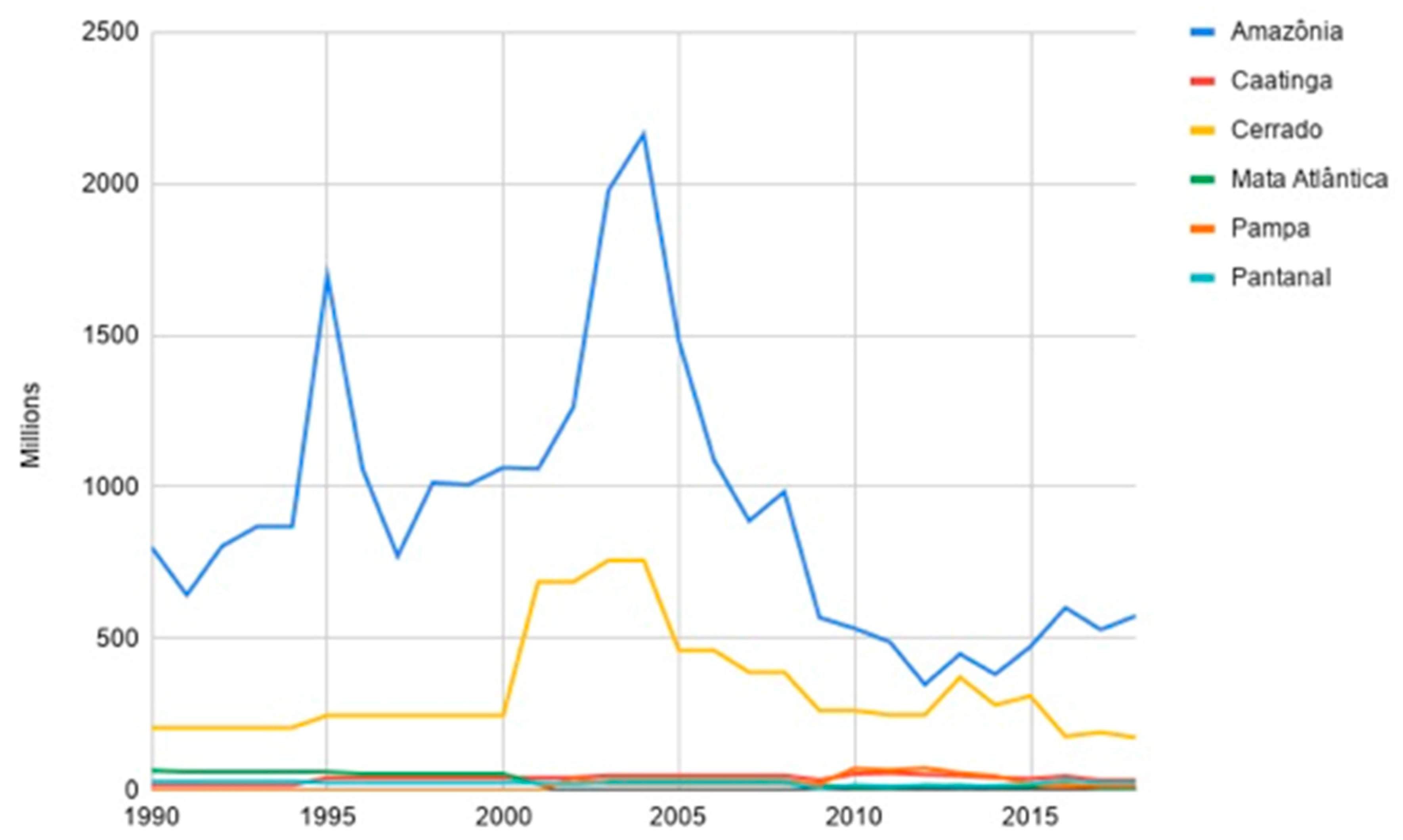7.390/2010 established an 80% reduction of deforestation in the Amazon biome in relation to the average verified between 1996 and 2005, and a 40% reduction of deforestation in the Cerrado Biome in relation to the average between 1999 and 2008 [15]. At the close of the 23rd Conference of the Parties (COP 23), the government informed the international community of a 16% reduction of deforestation in the country; this information is confirmed in the survey results. However, the results also show that deforestation in the Amazon remains the main responsible for the high CO₂ emission in Brazil, followed by deforestation in the Cerrado as shown in Figure 2.

When analyzing the correlation of economic activities and CO₂ emissions in Brazil, it is observed that the main emissions come from the change in land use and the agricultural sector, as shown in

Table 4. Correlation of economic activities and GHG emissions from 1970–2018.

Activities	Emissions			Activities	Emissions			Activities	Emissions
	CH4	CO2	N2O		CH4	CO2	N2O		CH4	CO2	N2O
TCSNF	0.715	0.248	0.811	L	0.722	0.415	0.789	CEP	0.424	0.086	0.478
SP	0.348	0.102	0.415	ADA	0.719	0.959	0.695	ONGP	0.061	0.098	−0.143
AP	0.413	0.129	0.49	ADCa	0.014	−0.068	0.057	HES	0.373	0.11	0.405
SCP	0.386	0.116	0.453	ADCe	0.396	0.534	0.299	GS	0.5	0.131	0.552
BP	0.828	0.453	0.822	ADAF	0.266	0.315	0.288	LPGS	0.506	0.15	0.559
MP	0.624	0.187	0.662	ADPamp	0.872	0.98	0.736	FOS	0.345	0.252	0.375
CP	0.592	0.198	0.681	ADPant	−0.017	0.565	0.013	DOS	0.639	0.255	0.696
SoyP	0.618	0.353	0.676	TLUC	0.519	0.913	0.473	TIP	0.493	0.167	0.522
BCH	0.928	0.591	0.879	AAP	0.905	0.856	0.267	IPPM	0.499	0.083	0.486
DCH	0.679	0.259	0.695	STP	0.346	0.212	0.248	TW	0.499	0.083	0.486
TA	0.627	0.193	0.703	AIP	0.151	0.548	0.123

. In the agricultural sector, emissions are due to the activities of beef cattle herd and beef production, which emit large amounts of methane (CH₄) through enteric fermentation (also known as rumen fermentation) of animals, followed by increased consumption of synthetic nitrogen fertilizers in the soil with increasing oxide emissions nitrous (N₂O) in the atmosphere. However, it is the change in land use that has the greatest correlation with CO₂ emissions. Note in Table 4 that deforestation in Pampa, one of the six Brazilian biomes located in the state of Rio Grande do Sul, has a strong correlation with CO₂ emissions in that state, whereas deforestation in the Amazon forest also reveals a strong correlation with CO₂ emissions between all states that have the Amazon rainforest (Mato Grosso, Pará, Rondônia, Maranhão, Tocantins, Amazonas, Roraima, Acre and Amapá). The annual average of deforestation in the Amazon was approximately 155,857.65 ha and in the Pampa approximately 35,245.55 ha.

In order to better observe GHG emissions, it is presented the dispersion graph (Figure 3), which shows the degree of relationship between land use change and CO₂ emissions in each Brazilian state.

The dispersion diagram in Figure 3 shows that there is a strong correlation between land use change and CO₂ emissions in the states of Mato Grosso (MT), Pará (PA), Goiás (GO), Minas Gerais (MG), Rondônia (RO), Amazonas (AM), Bahia (BA), Rio Grande do Sul (RS), Tocantins (TO) and Mato Grosso do Sul (MS). The main sources of emissions in Mato Grosso, Pará and Rondônia are deforestation, with the state of Mato Grosso being the largest emitter per capita. CO₂ emissions from land use change result from deforestation, variations in the amount of carbon in plant biomass, soil and CH₄ and N₂O emissions, as an outcome from burning biomass in soils. The states with high CH₄ emissions from bovine enteric fermentation descendant from animal manure management are the states of Minas Gerais (MG), Goiás (GO), Mato Grosso (MT), Pará (PA) and São Paulo (SP). 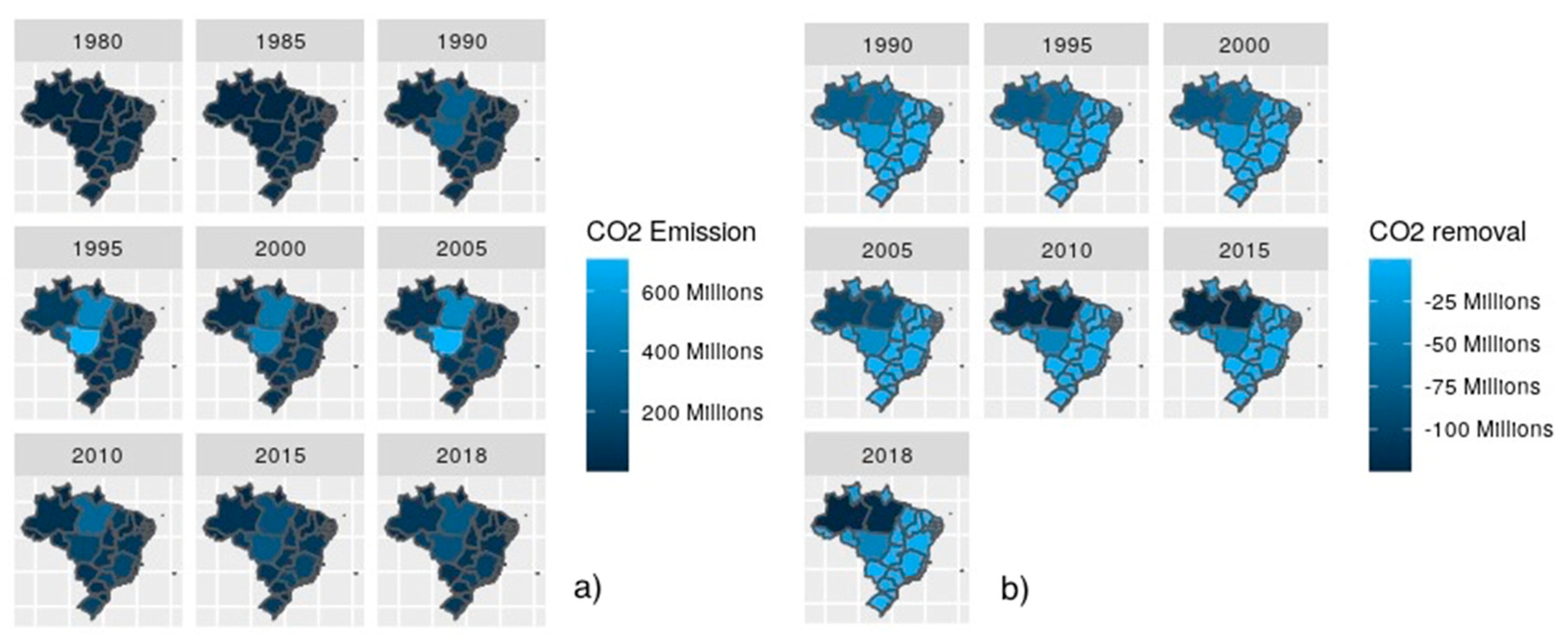In addition, N₂O emissions from bovine enteric fermentation, application of nitrogen fertilizers and fertilizer in the soil, and the cultivation of irrigated corn that also emits methane, were higher in the states of Minas Gerais (MG), São Paulo (SP), Goiás (GO), Paraná (PR) and Mato Grosso (MT). Emissions and removals of carbon dioxide (CO₂) in tons can be seen on the map in Figure 4.

Note that removals of carbon dioxide from the soil have been verified since the 1990s, with more expressive results since 2005 and 2010. The removals come from reforestation, growth of secondary vegetation, as well as areas of forest and native vegetation contained in Indigenous Lands and the National System of Nature Conservation Units, since they aim to fulfill relevant ecological, economic and social functions. The greatest CO₂ removals are seen in the states of Amazonas, Pará and Mato Grosso. These results confirm the need to have and maintain established environmental protection policies. With the implementation of PPCDAm and PPCerrado, it was possible to achieve the results verified since 2005.

For the multilevel regression analysis, the data was transformed into logarithms, which resulted in data with a normal distribution. In this case, the logarithm is applied to both the dependent variable (CO₂) and the independent variables, which results in a model known as log-log [21]. Before applying the multilevel model, multiple regression analysis was used as a strategy to exclude not significant variables and variables containing VIFs greater than 5. With this analysis, Equation (10) was obtained to explain CO₂ Brazilian emissions:

$$\log ({\mathrm{CO}}_2)={\mathsf{\beta }}_0+{\mathsf{\beta }}_1\log \left(\mathrm{TLUC}\right)+{\mathsf{\beta }}_2\log \left(\mathrm{BP}\right)+{\mathsf{\beta }}_3\log \left(\mathrm{SoyP}\right)+{\mathsf{\beta }}_4\log \left(\mathrm{TIP}\right)+{\mathsf{\beta }}_5\log \left(\mathrm{SP}\right)$$

(10)

The model proposed by multiple linear regression (Equation (10)) to explain CO₂ emissions suggests the following variables: land use and change (LUC), beef production (BP), soy production (SoyP), total industrial production (TIP) and sugar production (SP). The model was analyzed using only the total variable of land use change that showed an R² of 0.4. The model with the land use and change and beef production showed an R² of 0.65 and the model in Equation (10) showed R² of 0.71, that is, soy production, industrial production and sugar production collaborated with only 0.06 to improve the model; however, it was the best possible model found.

The results of the regression of the model estimated in Equation (10) showed statistical significance (F = 137) with a p-value less than 0.00001. The model presented the value of R² equal to 0.71, indicating that approximately 71% of the logarithmic variation explains the CO₂ variable, all coefficients of the independent variables are statistically significant, as shown in

Table 5. Multiple Regression Model for Selection of Variables.

Variable	Estimate (β)	Std. Error		Pr(>|t|)
(Intercept)	9.80626	0.37629	26.06	<2 × 10−16 ***
Log (TLUC)	0.37259	0.02446	15.23	<2 × 10−16 ***
Log (BP)	0.19143	0.03231	5.924	9.27 × 10−9 ***
Log (SoyP)	0.05742	0.01184	4.852	2.05 × 10−6 ***
Log (TIP)	0.04389	0.01045	4.199	3.62 × 10−5 ***
Log (SP)	0.04106	0.01731	2.372	0.0184 *

Signif. codes: 0 ‘***’ 0.001 ‘*’ 0.05 ‘.’ 0.1 ‘ ’ 1.

.

As the model assumes, all β coefficients were highly significant, and only the β5 coefficient related to sugar production was less than 0.05, while the other variables were less than 0.001; the average of the errors was approximately zero and its distribution is close to the normality pattern as shown in Figure 5.

In the multilevel regression model [24], it was considered the experiment with two levels: the first level refers to annual CO₂ emissions and the second level refers to Brazilian states. The null model was adjusted, as it provides the information of the intra-class correlation that analyzes the amount of explained variance, which is defined by the characteristic of the states, as shown in Equation (4).

When estimating the null model, it was found that 93.7% of the variation in CO₂ emissions can be attributed to differences between states. An assumption for this high number is the large difference in CO₂ emissions between states. That is, while the states of the North and Midwest had large volumes of emissions, other states showed comparatively low values, due to the characteristics of the states. However, the variability that is interesting to know is the one obtained from a model that controls the influence of economic variables (extra state variables) on the performance of CO₂ emissions, since the allocation of the variables economic activities of the states are not random. The model parameters are shown in

Table 6. Inclusion of the TLUC variable with the Year variable.

Models:	Df	AIC	BIC	logLik	Deviance	Chisq	Chi Df	Pr(>Chisq)
CO2~1 + (1|UF)	3	632.40	646.36	−313.20	626.40
CO2~TLUC + (1|UF)	4	589.89	608.51	−290.94	581.89	44.510	1	2.53 × 10−8 ***
CO2~TLUC + (TLUC|UF)	6	−17.18	10.75	14.59	−29.18	611.066	2	<2.2 × 10−6 ***
CO2~TLUC + Year + (TU|UF)	7	−767.83	−735.25	390.92	−781.83	752.655	1	<2.2 × 10−16 ***
CO2~TLUC + Year + (TLUC + Year|UF)	10	−830.78	−784.23	425.39	−850.78	68.945	3	7.18 × 10−12 ***
CO2~TLUC + BP + (TLUC|UF)	7	−262.13	−230.90	138.063	−276.13	145.123	1	<2.2 × 10−16 ***
CO2~TLUC + BP + (TLUC + BP|UF)	10	−459.41	−414.79	239.704	−479.41	203.280	3	<2.2 × 10−16 ***
CO2~TLUC + SoyP + (TLUC|UF)	7	−318.66	−289.05	166.332	−332.66	137.32	1	<2.2 × 10−16 ***
CO2~TLUC + SoyP + (TLUC + SoyP|UF)	10	−500.75	−458.44	260.374	−520.75	188.09	3	<2.2 × 10−16 ***
CO2~TLUC + TIP + (TLUC|UF)	7	−359.51	−327.46	186.757	−373.51	346.730	1	<2.2 × 10−16 ***
CO2~TLUC + TIP + (TLUC + TIP|UF)	10	−575.05	−529.26	297.526	−595.05	221.537	3	<2.2 × 10−16 ***
CO2~TLUC + SP + (TLUC|UF)	7	−64.570	−34.874	39.285	−78.570	342.381	1	4.88 × 10−6 ***
CO2~TLUC + SP + (TLUC + SP|UF)	10	−167.229	−124.807	93.614	−187.229	1.086.59	3	<2.2 × 10−16 ***

Signif. codes: 0 ‘***’ 0.001 ‘.’ 0.1 ‘ ’ 1.

.

Several models were built using the variables found in the multiple regression model of Equation (9), in addition to including the variable year, to verify trends in CO₂ increase or decrease. The first adjusted model was the null model CO₂~1 + (1|UF)). The second adjustment was the model with the variable land use change (TLUC) in the fixed part of the multilevel model (CO₂~TLUC + (1|UF)). In the third model, the variable land use change (TLUC) was included in the random part (CO₂~TLUC + (TLUC|UF)). Comparing the first three models in Table 6, it is possible to observe that they are statistically different according to the observed p-value of the likelihood ratio test (Pr(>Chisq)). However, the best model was the one that presented the variable land use and change (TLUC) both in the fixed part and in the random part (CO₂~TLUC + (TLUC|UF)), as it presented lower indicators AIC and BIC.

Testing the variable year in the model both in the fixed part and in the random part, it was observed that despite presenting significance, there was no improvement in relation to the model with the variable TLUC; therefore, the variable year was excluded. All variables (BP, SoyP, TIP, SP) were tested both in the fixed part and in the random part, with the variable TLUC; however, none showed better results. This is due to the difference in economic activity in each Brazilian state.

Thus, the model that best explains the CO₂ emissions was selected, presented in Equation (11). Using the notation from Raudenbush and Bryk [22], this model uses the TLUC variables in both the Random effects and Fixed effects.

$$\log \left({\mathrm{CO}}_{2\mathrm{ij}}\right)={\mathsf{\gamma }}_{00}+{\mathsf{\gamma }}_{10}\log \left({\mathrm{TLUC}}_{\mathrm{ij}}\right)+{\mathrm{u}}_{0\mathrm{j}}+{\mathrm{u}}_{1\mathrm{j}}\log \left({\mathrm{TLUC}}_{\mathrm{ij}}\right)+{\mathrm{e}}_{\mathrm{ij}}$$

(11)

where i is the annual CO₂ emission and j is the State, ${\mathsf{\gamma }}_{00}$ and ${\mathsf{\gamma }}_{10}$ are the parameters related to the fixed effects, ${\mathrm{u}}_{0\mathrm{j}}$ is the random error component of the state level and ${\mathrm{u}}_{1\mathrm{j}}$ is associated with the slope coefficient that associates the part of the random effect and ${\mathrm{e}}_{\mathrm{ij}}$ is the residue of the CO₂ emission level.

Table 7. Multilevel model parameters.

Random Effects:
Variable	Variance	Std.Dev.	Corr
UF(Intercept)	15.128	3.889
TLUC	0.147	0.383	−0.98
Residual	0.04	0.2
Fixed Effects:
Variable	Estimate	Std. Error	t-value
(Intercept)	13.72309	0.76794	17.87
TLUC	0.31905	0.07531	4.236

presents the results of the selected model.

Analyzing the results in Table 7, the random effect presents the estimate of variance and the standard deviation of the effect associated with States with a variance of 15.128 and standard deviation of 3.889. It also presents the variance between the iteration of the variable TLUC and State in the random effect with 0.147 and the variance of the residue with 0.04. This variance represents the values that cannot be identified by the variables, so it is noticed that the correlation associated with the variance between State and TLUC has high values of −0.98. The fixed model estimates have the same interpretation as the linear regression model, remembering that in this case the values refer to the log of the variables. It is noticed that the coefficient related to the intercept has a value of 13.72 and the variable TLUC has a positive value of 0.319, that is, the TLUC contributes to the increase in CO₂ emissions. The parameters can be interpreted as follows: when the TLUC value = 1, the log value (TLUC) = 0, the expected value for CO₂ is equal to exp (13.723); when the TLUC mean value increases by 1%, it is expected a variation of 0.319% in the CO₂ variable.

This interpretation occurs because of the application of the transformation of variables into logarithmic. This same interpretation can be used for the data disaggregated in states of the multilevel model. The results of the model coefficients per state unit are presented

Table 8. Multilevel model coefficients by state.

UF	Intercept	TLUC	UF	Intercept	TLUC
AC	9.889	0.696	PB	14.742	0.128
AL	16.308	−0.081	PE	17.841	−0.105
AM	8.332	0.853	PI	9.478	0.662
AP	9.894	0.663	PR	18.194	−0.033
BA	13.014	0.429	RJ	18.179	−0.073
CE	17.979	−0.092	RN	15.21	0.075
DF	14.901	0.088	RO	10.66	0.67
ES	17.626	−0.121	RR	8.145	0.847
GO	12.142	0.52	RS	15.784	0.253
MA	8.967	0.768	SC	18.639	−0.156
MG	14.678	0.347	SE	16.991	−0.174
MS	13.496	0.404	SP	20.196	−0.152
MT	9.341	0.78	TO	9.526	0.703
PA	10.372	0.713

.

Table 8 shows the coefficients of the intercept and the slope of the curve within the states; note that both are random. In this case, the intercept represents the amount of CO₂ explained by the characteristic of the states, which is due to the fact that each state has different economic activities, that is, some are more industrial and others are more agricultural. It can also be noted that some states have negative slope coefficients, which is due to the fact that these states do not have high TLUC numbers and even in relation to CO₂ emissions when compared to other states with positive slope coefficients, as the states that are part of the Amazon region. The states with the highest CO₂ emissions are those with the largest hectares of deforestation.

The histogram of the model’s residual (Figure 6) showed an approximation of a normal distribution, which shows that the model is well adjusted, presenting good quality.

It can also be seen in

Table 9. Average growth rate for the period in Brazil.

Period	Beef Production (%)	Soy Production (%)	Sugar Production (%)	Industrial Production (%)	Total Land Use and Change (%)	CO2 Global Warming Potential (%)
1990–2004	11.55	6.73	9.26	12.95	6.02	6.25
2004–2010	2.89	5.61	4.77	3.57	−15.53	−11.17
2010–2018	1.7	6.97	1.99	1.17	−2.98	−0.34

that, in the period from 1990 to 2004, where there was an increase in CO₂ emissions in the country (Figure 2), there was also an increase in the number of deforestation (Total land use and change) and the other production variables (Beef Production, Soy Production, Industrial Production). However, in the period from 2004 to 2010, a sharp reduction of deforestation can be observed, followed by a fall in CO₂ emissions, while in the period from 2010 to 2018, the rate of production growth despite lower continued to grow, and the variables of deforestation and CO₂ emissions continued to decrease, once again affirming the importance of commitments to the Environmental Protection Policy. Note that the results presented in Table 9 corroborates with the information released by the government; in fact, there was a decrease of approximately 16% in the mean rate of deforestation in the period from 2004 to 2010, and after this period, it continued to show a rate of reduction of the deforestation by 2018.

The results obtained in this study are distinguished from previous studies and contribute to fill a gap in the literature. First, the share of economic activity variables (Table 1) was not used in any other study, together with the CO₂ emission variable. Secondly, unlike the classical regression models that consider both the intercept and the slope coefficients to be fixed, the multilevel linear models naturally and parsimoniously incorporate the hierarchical or grouping structure under study, treating the intercept and the coefficients slope as random variables. They show that the structure for each group (states) should not be the same since the random effect model demonstrates that there are different characteristics in each state that contribute to CO₂ emissions. However, the model shows that the most significant extra state variable shared between the groups is the change in land use (Table 8), the parameters estimated by the tested models are more accurate, since all available information is considered.

Many studies have been conducted in order to study the relationship between different variables with CO₂ emissions. Huaman and Jun (2014) claim that CO₂ emissions are driven, in large part, by economic and population growth [25]. Al−Mulali et al. (2015) address economic growth and energy consumption as factors that impact long-term CO₂ emissions [26]. Mendonça et al. (2020) investigated the impact of renewable energy, GDP, and population on CO₂ emissions of the 50 largest economies from 1990 to 2015 [27]. Alam, Md Mahmudul, et al. (2016), Riti et al. (2017), Li et al. (2017), Ahmad et al. (2018) and Dong, K.Y. et al. (2018) corroborate that economic growth and energy consumption influence CO₂ emissions [28,29,30,31,32].

However, an analysis was not found in the literature that considered the variables of economic activities, such as, for example, the land use change with the variable CO₂ emission. In Brazil, we have identified a different characteristic in CO₂ emissions; while in many countries, CO₂ emissions are explained by economic and population growth and by the production of electricity, in Brazil the variable that best explains CO₂ emissions is the change in use of the land, with its deforestation. This information confirms the importance of environmental policies in preventing and or mitigating CO₂ emissions in Brazil.

5. Conclusions

This study investigates the main environmental protection and climate change mitigation policies adopted in Brazil and uses the multilevel regression modeling technique to investigate the relationship between economic activity variables in relation to CO₂ emissions over the years 1970 to 2018 in all Brazilian states. Brazil is the fifth largest country in the world, presenting in its vast territorial extension a diversity of ecosystems that form six biomes (Amazon, Cerrado, Caatinga, Atlantic Forest, Pantanal and Pampa). These biomes will be affected by climate change. To try to reduce climate change, Brazil developed a political structure for environmental protection and mitigation of climate change and, under the Paris Agreement, made a commitment to reduce its greenhouse gas emissions by 37% until 2025, compared to data recorded in 2005, and to reduce carbon emissions by 43% until 2030.

With the multiple regression analysis, it is seen that some variables of economic activity are related to CO₂ emissions. However, when these variables were applied in the multilevel regression model, it was observed that the characteristics of the states have significant differences and that the only variable that helps explain CO₂ emissions in Brazilian states is the change in land and forests use variable. This means that when there is a reduction in land and forests use, there is also a reduction in CO₂ emissions. Likewise, we can say that large volumes of CO₂ emissions that occur in certain regions of the country, such as in the northern and central western regions of the country, occur due to the change in land and forest use, which in this case is deforestation. This result can be seen in the dispersion diagram in the state of Mato Grosso and the state of Pará, which were the main responsibility holders for Brazil’s CO₂ emissions (Figure 3).

According to the National Plan for Adaptation to Climate Change (PNA), South America is at risk of extinguishing 23% of its species due to climate warming. The most affected biomes will be the Amazon and the Cerrado, where the native vegetation will suffer from the severe changes caused by the increase in temperature. In the Amazon biome, a large part of the forest is in the territory of the Brazilian states and has an important relevance for the normalization of the climate of the entire planet. The biome’s vegetation has the function of absorbing carbon dioxide emissions from the atmosphere and acting for the balance in periods of rain throughout South America.

The Cerrado biome occupies almost 25% of the Brazilian territory in a region that still has lower rates of economic development. The inequality that exists in the Cerrado needs to be analyzed. The biome will also suffer from periods of drought, which will occupy a large part of the year contributing to fires, in addition to reducing the number of trees that are important regulators of temperature and suck the water that is in the soil. The Cerrado is one of the largest water distributors for the main hydrographic basins in Brazil, being responsible for supplying eight of them. Therefore, river basins may be affected by climate change.

The results obtained through the random model showed that CO₂ emissions have the same behavior as the land use change (TLUC) timeline and that public policies, along with actions by society and the private sector, were fundamental to the reduction of CO₂ emissions and in the change of land and forests use (TLUC) from the year 2004 that continued until the year 2010. From this year, it followed a trend of stability in the emission of CO₂ and TLUC. Another important characteristic is that even with a drop in the number of deforestation, the production variables continued to rise for these same regions, which demonstrates that there may be an increase in production even though the numbers of deforestation and CO₂ emissions are decreasing. That information strengthens the Action Plan for Prevention and Control of Deforestation in the Legal Amazon (PPCDAm), the Action Plan for Prevention and Control of Deforestation and Burning in the Cerrado (PPCerrado), and the Low Carbon Agriculture Program (Plan ABC) as the main strategies for reducing CO₂ emissions and the development of the productive sector, mainly for the development sustainable agriculture.

The results obtained in this study are distinguished from previous studies, as while in many countries CO₂ emissions are explained by economic and population growth and by the production of electricity [22,25,26,27,28,29,30,31,32], in Brazil the variable that best explains CO₂ emissions is the change in use of the land, with its deforestation. This information confirms the importance of environmental policies in preventing and or mitigating CO₂ emissions in Brazil.

However, in 2019, with the transfer of forest management from the Ministry of the Environment to the Ministry of Agriculture and the extinction of the Secretariat for Climate Change and Forests who was responsible for coordinating the implementation of emission reduction policies, and for the plans for prevention and control of deforestation in the Amazon (PPCDAm) and the Cerrado (PPCerrado), the environmental protection policies and their action plans are undefined. The Ministry of Agriculture is now competent to formulate strategies, policies, plans and programs for the management of public forests.