Conceptual Framework for Biodiversity Assessments in Global Value Chains

Abstract

Land use and land use change are among the main drivers of the ongoing loss of biodiversity at a global-scale. Although there are already Life Cycle Impact Assessment (LCIA) methods to measure this impact, they are still rarely used by companies and municipalities in the life cycle assessment of products and processes. Therefore, this paper highlights four main requirements for a biodiversity methodological framework within LCIA in order to facilitate biodiversity assessments: first, to consider the global uneven distribution of biodiversity and its risks with respect to vulnerability and irreplaceability; second, to account for the need to regionalize the impacts of land use; third, to consider the specific impacts that different land use types have on biodiversity; and fourth, to analyze the biodiversity impacts of different land use management parameters and their influence on the intensity of land use. To this end, we provided a review of existing methods in respect to conformity and research gaps. The present publication describes the development of a new methodological framework that builds on these requirements in a three-level hierarchical framework, which enables the assessment of biodiversity in LCA at a global-scale. This publication reveals research gaps regarding the inclusion of proactive and reactive conservation concepts as well as methods of land management into LCIA methodology. The main objective of this concept paper is therefore to describe a new methodological framework for the assessment of biodiversity in the LCA that could fill some of the research gaps, including compilation and suggestion of suitable data sets. The conclusion discusses both the benefits and limitations of this framework.

1. Introduction

Relevance and General Context

When Silent Spring was published in 1962, it encouraged the creation of a global conservation movement which began to tackle the manifold ecological challenges. Today, the scientific community has identified nine pressing global environmental problems such as ocean acidification, chemical pollution, the anthropogenic effects on the nitrogen cycle, and the climate crisis, which is receiving the most media attention [1,2,3,4]. Especially one of the planetary boundaries, which decisively kicked-off environmental studies, public concerns, and regulatory initiatives, exceeds, by far, the safe operating space—the loss of biodiversity [4]. According to the Millennium Ecosystem Assessment, mankind has caused the loss of biodiversity and contributed to the extinction of species at an unprecedented rate [5]. Since the extinction rate of earth’s species is far above the natural background extinction rate, scientists also call the current loss of biodiversity the sixth major mass extinction [6,7,8,9,10]. In this respect, approximately two-thirds of the global biodiversity crisis is due to direct anthropogenic land use activities [11]. This accumulation of human influences could even cause a cascade effect which would increase the extinction rate at an uncontrollable rate [12]. Considering the urgency to mitigate this development, a warning has been issued on the current biodiversity crisis signed by more than 1700 concerned scientists [13].

The rapid loss of biodiversity is not only an environmental concern but has also a decisive impact on the economy and all of society. Developing countries as well as highly industrialized countries are fundamentally dependent on ecological stable conditions [14] and increasingly recognize the value of functioning ecosystems, hence the re-introduction of former locally extinct species [15]. The most prominent beneficial function of biodiversity is termed, in socioeconomic terms, ecosystem services. Such services include among others nitrogen fixation, the fixation of GHG emissions, soil protection, a cooling effect on urban microclimates and, therefore, reducing stress on materials such as concrete, an increase in air purification which mitigates pulmonary diseases, and pollination. In order to provide this multitude of services, ecosystems need a diversity of taxa to enable complex ecological interactions. Also it has been shown that several ecosystem functions (also called ecosystem multifunctionality) significantly increase with a higher biodiversity rate [16,17]. When it comes to estimating the financial worth of such ecosystem services, the Natural Capital Protocol compares biodiversity with a stock from which companies and societies benefit from intact and healthy ecosystems [18]. The primary sector in particular is highly dependent on biodiversity and ecosystem services through their business models in agriculture and forestry; secondary and tertiary sectors highly benefit from ecosystem services and suffer from the lack of hereof. Examples of collapsed ecosystems which are no longer able to provide the required ecosystem services serve as a warning of the high follow-up costs [19].

In many countries the biodiversity crisis, e.g., coral bleaching, has led to national response programs to tackle the rapid loss of biodiversity which is seen as a national treasure and a guarantee for a continuous flow of tourism [20]. The long-assumed trade-off between economic growth and environmental protection does not hold to be true any longer (if it ever was). In fact, most socioeconomic activities depend on sound ecosystems with a rich biodiversity. Increasingly more companies and municipalities are aware of their dependency but also on their negative impacts on biodiversity due to waste, disturbances or changes in habitats and land use. A negative impact on biodiversity further increases the risks with their suppliers or customers as part of the supply chain, higher costs for resources, increasing resource scarcity, or official national and international regulations [18]. The awareness that basically all socioeconomic activities have a disturbing impact on biodiversity, on which they also depend, makes the development of an instrument that is capable of quantifying the impacts on biodiversity and deriving recommendations to mitigate these negative effects a pressing priority [21].

Land use and land use change are considered to be amongst the main drivers of biodiversity loss; additionally, it can be shown that the intensity of land management and the choice of management practices have a considerable impact on biodiversity [22,23,24,25,26].

To assess land use impacts on biodiversity Life Cycle Assessment (LCA) is the main instrument used by companies to assess the effects of materials, products and processes throughout the entire value chain. A global study on the use of LCA in industry however shows that, despite the above-mentioned relevance, companies rarely consider the loss of biodiversity in their assessments [27]. This could be due to the fact that current biodiversity assessment methods still have some limitations in their application.

Some of these limitations have been described in several review studies on biodiversity methods in LCIA and are therefore not the subject of this publication. These include the type of biodiversity indicators used [28,29,30,31], impact and pressure models [28,30,32], the coverage of impact pathways, the acceptance of interest groups [33], spatial differentiation [34] and spatial correlation [35], or the choice of a reference system [36]. This study focuses on the inclusion of existing conservation schemes into LCIA methods, the consideration of reactive and proactive conservation approaches, as well as the coverage of current methods with regard to land use types, intensities, and management parameters. As we can show in this publication, there are still research gaps with regard to these aspects.

The main objective of this concept paper is therefore to describe a new methodological framework for biodiversity assessment in LCA that could close some of the research gaps, including the compilation and suggestion of suitable datasets. In the end, it discusses its advantages as well as its limitations.

2. Requirements for a Biodiversity Methodology in LCA

2.1. Requirements—From an Ecological and Conservation Perspective

Since the term ‘biodiversity’ is genuinely from the biological-ecological field as well as from conservationists, it is prudent to consider scientific requirements and definitions from these fields in order to combine the know-how of LCA, biology, and ecology. The next subchapter then deals with the technical requirements from a life cycle perspective. In order to make ‘biodiversity’ applicable to LCA one can identify two (simplified) main requirements. The first deals with the different levels of biodiversity while the second with the uneven distribution of and threats to biodiversity around the world.

As regards definitions of biodiversity, the term is often used as a buzzword in politics and social contexts. According to ref. [12], there are more than 85 different definitions of biodiversity. However, most scientists agree on the definition of the Convention of Biological Diversity (CBD): “Biological diversity means the variability among living organisms from all sources including, inter alia, terrestrial, marine and other aquatic ecosystems and the ecological complexes of which they are part; this includes diversity within species, between species and of ecosystems” [37]. As the CBD notes, the richness of ecological processes is important for the protection of biodiversity and it can be described in terms of three aspects: genes, species and ecosystems. However, it is important to emphasize that—like all classifications—it is a simplification. Also, all aspects are interconnected: genes define a species and different species form an entire ecosystem. If one considers all three aspects in a Life Cycle Impact Assessment (LCIA) methodology in view of this interconnectedness, a kind of double counting is inevitable. According to ref. [28], there is no method for assessing biodiversity in LCA that meets those multifaceted aspects [28]. Most of the existing methods focus either on the species or on the ecosystem level. This is mainly justified by the fact that the genetic level can usually only be measured on a small scale (laboratory) or via proxies. However, the genetic scale is crucial because it is important for the evolutionary adaptability of the species that make up a community, a population and the entire ecosystem. Especially in times of global change and mass extinction, the adaptation of species, as defined by genetic selection in response to the changing environment, is of utmost importance. One way to consider the genetic level in LCA is to evaluate the phylogenetic diversity of species. Phylogenetic diversity describes the evolutionary relationship between species—and therefore the richness of the gene pools between species. Hence, the conservation of phylogenetic diversity (here phylogenetically different species) offers greater potential for adaptation to global change [38]. In addition, a wider variety of phylogenetic groups are more likely to offer more ecosystem functions, because closely related species tend to occupy similar niches and therefore similar ecosystem functions [39,40]. The integration of phylogenetic information into biodiversity assessments is increasingly becoming common in the life and conservation sciences while still being in its infancy in global land use assessments and LCA [38]. However, especially in view of the unpredictable effects of the ongoing global crisis, the protection of the evolutionary potential of species is the best ‘insurance’ to increase adaptability [41].

As for the second requirement, there are general macroecological patterns of species richness and distribution, with the highest concentration of terrestrial species at the equator and alternating diversity towards the poles. As a result, biodiversity is not evenly distributed across the globe. In addition, not only is biodiversity unevenly distributed, but it is also faced with uneven risks worldwide. This unequal distribution of species, ecosystems, and threat levels makes it necessary to prioritize and evaluate areas for the conservation of biological diversity [42]. Extensive research has been undertaken by scientists and NGOs to prioritize global areas where the protection of biodiversity is most urgent, see refs. [43,44,45,46,47,48,49,50,51,52]. Ref. [53] reviewed various global biodiversity conservation schemes and found that the following categorization is used in nature conservation science to assess regions for their biodiversity risk: irreplaceability and vulnerability [42,53]. The criteria for irreplaceability are the number of endemic species, taxonomic uniqueness, unusual phenomena, the rarity of important habitat types, and the number of species (richness). The criteria for vulnerability are the level of threat (usually based on the IUCN red list) and the amount of habitat lost. Vulnerability is then labeled as high (for reactive approaches) or low (for proactive conservation) depending on the degree of habitat degradation—while both are esteemed as worth protecting [42,53]. Thus, these requirements deal with the development of a global biodiversity risk map that is able to depict the quality and quantity of biodiversity worldwide.

2.2. Requirements—From an LCA Perspective

The general purpose of a LCA is to compare different products, materials, or production processes with alternatives in order to identify those with the lowest environmental impact during their entire life cycle, hence optimizing existing products and processes. In respect to biodiversity such an assessment should be able to quantify biodiversity at a global-scale depending on three factors [54]:

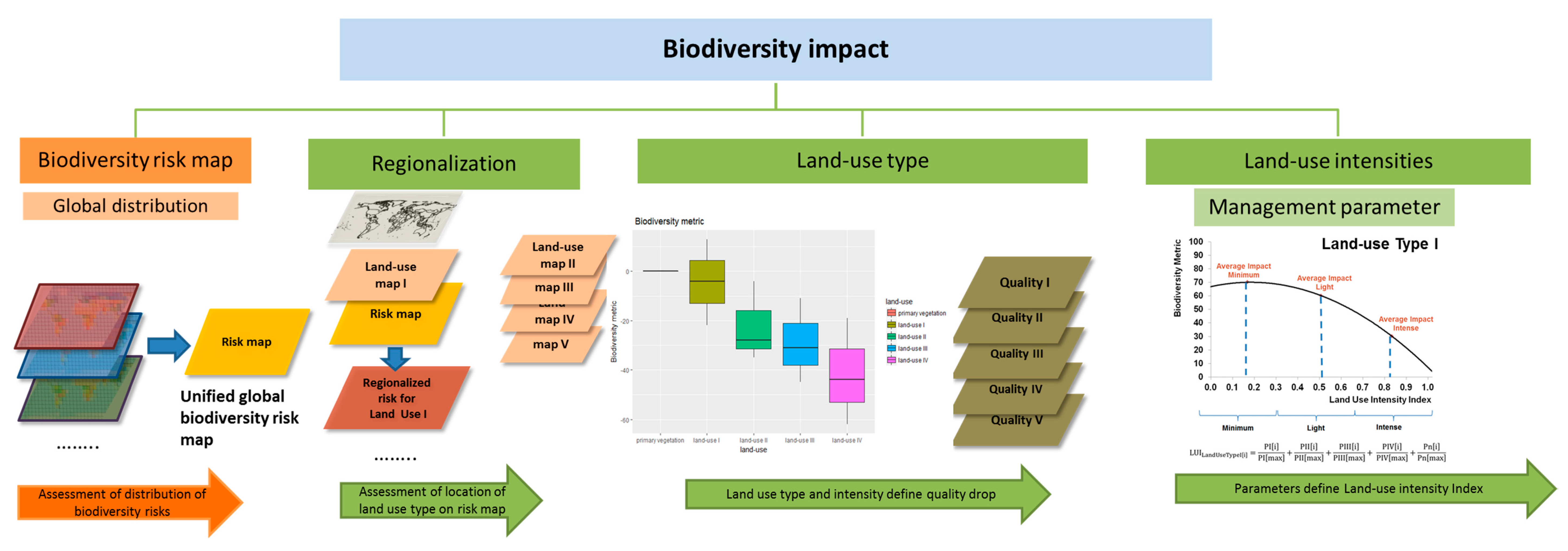
• First, the factor of regionalization. This factor reflects the fact that biodiversity is not evenly distributed across the world and neither are the threats to biodiversity, e.g., there are places with high pressure on biodiversity, places with low anthropogenic disturbances or areas with a high number of species [55,56]. This makes it necessary to have a regionalization factor that can distinguish between different locations of land use, for example: Is it better to use resources from Spain in terms of biodiversity than rather, the same resources, from South Africa? The next step should further pinpoint the location in order to evaluate the impact on a specific region within a country. Here, some regions may still be intact and contain endangered or endemic species; while other regions may already be off-balance, and therefore land use in that region would have fewer negative effects [24,53]. If companies or municipalities want to mitigate their negative impact within their supply chains, it may prove beneficial for biodiversity to source materials from another location or to move the land use to another area.
• Second, the type of land use. A well-developed methodology should be able to assess different types of land use for alternative materials within a production chain [54]. Such land use types include forestry and plantations, agricultural land use, pasture, urban areas, or mining sites. For example, the use of the material ‘wood’ (land use type: forestry) should be comparable to the use of ‘banana leaves’ (land use type: plantation) for one-way plates. In addition, it must be taken into account whether these effects differ depending on the location. This question is especially relevant for the design of new products where different materials and alternative resources can be compared and taken into account in time.
• Third, the degree of land use intensity and suitable management parameters. Depending on the management practices applied in an area, land use has different intensities [22]. It should be possible to distinguish between land use intensities and to quantify their diverse impacts on biodiversity. In this respect, for example, extensive agriculture can be compared with intensive agriculture. Such management practices include the amount of used fertilizers and pesticides, the sampling of exotic or native trees, and the density of livestock. An assessment should quantify which land use practices have higher impacts on biodiversity and identify the influence of specific management parameters. Recommendations should be made as to which land use practices could be changed in order to minimize negative impacts on biodiversity and, if possible, increase positive effects.
• A biodiversity assessment method should therefore take into account the three above-mentioned levels in order to assess the impact on biodiversity [54,57], compare different sites and types of land uses, and provide recommendations for careful land use practices as well as alternatives. A similar conceptual model has been recommended by the IPCC for assessing land use impacts on climate change [58].

3. Biodiversity Impact Assessment in LCA

The main scope of this section is to summarize and compare the similarities and differences between existing biodiversity methods in LCIA and other disciplines such as biodiversity conservation science or ecology. These include the use of the concepts of reactive and proactive approaches, as well as irreplaceability and vulnerability for biodiversity assessments (Section 3.1), the associated regionalization of land use impacts (Section 3.2.1) and the assessment of land use and land management methods (Section 3.2.2 and Section 3.2.3). In all subsections, a brief overview is given of the state of the art with regard to existing LCIA methods on biodiversity and their current gaps. This is followed by the layout of the methodological framework and a description of how it contributes to closing some of the current gaps.

3.1. Biodiversity Risk Map

3.1.1. State of the Art and Research Gaps

As has been already explained, biodiversity is unevenly distributed around the world. It is therefore crucial to have a global biodiversity risk map that defines biodiversity as holistic as possible and indicates its distribution and risks around the world. Scientists and NGOs have carried out significant research to identify priority areas worldwide where the protection of biodiversity is most urgent, such as High Biodiversity Wilderness areas (HBWA) [43], Frontier Forests [47], Global 200 Ecoregions (G200) [45], Last of the Wild (LtW) [48], Endemic Bird Areas (EBA) [52], Centers of Plant Diversity (CPD) [51], Biodiversity Hotspots (BH) [44,59], and Crisis Ecoregions [46], among others.

According to ref. [53], all these global conservation schemes can be placed either in the context of irreplaceability or vulnerability, although some approaches are mixed. In either case, each biodiversity protection scheme has a different focus (either on specific taxa, threat level, or biodiversity level) and, so far, scientists and NGOs have not agreed on a common biodiversity protection scheme [42,53,60,61]. Moreover, most of these schemes do not take phylogenetic differences into account. A further gap exists in the underrepresentation of nonvertebrate species, such as insects or belowground biodiversity [53,62,63,64,65].

In LCIA methods, biodiversity risks are assessed based on research by ecologists, NGOs, and conservationists. Therefore, all LCIA methods can be classified in terms of irreplaceability or vulnerability according to [53]. However, there are still differences between the prioritization of biodiversity aspects in conservation science and LCIA methods. The majority of LCIA methodologies focus on aspects of high vulnerability (reactive approaches), with habitat loss as proxy for species loss or the level of ecosystem degradation [66,67,68,69,70,71,72,73,74,75,76,77,78]. Another common approach that gives priority to high vulnerability is the assessment of land use due to the occurrence of threatened species [66,69,74,75,79,80,81]. Herein, there is a higher risk if land use takes place in an area where endangered species live. Whereas methods using habitat loss as a proxy focus on high vulnerability (reactive approaches), and methods using hemeroby or related measures highlight areas with low vulnerability (proactive approaches). Yet, there are no LCIA methodologies that take into account already presented global conservation schemes such as intact forest landscapes, the last of the wild or High Biodiversity Wilderness Areas [43,82,83,84,85,86]. However, such areas are particularly important for assessing the impacts of land transformation on biodiversity, as it is better to transform and use already degraded land compared to intact ecosystems [43,82,83,85,86].

In the context of irreplaceability, species richness is the most common metric used in LCIA methods [30,71,72,79,80,81,87,88,89,90,91,92,93], which is followed by an assessment with regard to rare habitats or ecosystems [28,67,70,73,75,79,89,92]. Only few methods take into account the occurrence of endemic species [38,74,77,79,81]. And no method includes critical, irreplaceable biodiversity areas such as the Endemic Bird Areas, AZE sites, or Centers of Plant Diversity. There is also no methodology that includes further aspects such as areas with great migration routes or large species concentrations. However, they have been highlighted as critical for biodiversity and are therefore part of the Global 200 ecoregion conservation scheme [45]. Additionally, no method takes into account areas that are crucial for phylogenetically different species and genetic aspects. Whereas the majority of global conservation schemes prioritize and focus on endemism (high irreplaceability) [53]; most LCIA methodologies focus on vulnerability and only a few of them consider endemism at all.

Table 1. Life Cycle Impact Assessment (LCIA) biodiversity methods and irreplaceability and vulnerability.

											Reactive		Proactive
Author	Regionalization/Location	Land Use Type	Irreplaceability (i) Vulnerability (v)	Valuation	Biodiversity-Level	Number of Endemic Species	Taxonomic Uniqueness	Unusual Phenomena	Rare Habitats, Ecosystems	Number of Species (Richness)	Threat Level	Habitat Loss, (Degradation High)	Intact Habitat/Ecosystem
						Irreplaceability					Vulnerability
[87]		x	i	Richness	Species					x
[88]	x	x	i	Biomass production	Species					x
[94]		x	v	Hemeroby	Ecosystem								x
[89]		x	i	Richness, rare ecosystems	Species, Ecosystems				x	x
[66,95]		x	v, i	Threatened species, habitat loss (SARs)	Species					x	x	x
[79]		mining	v, i	Richness, threat, endemism, rare biotopes	Species, Ecosystems	x			x	x	x
[80]		x grassland, cropland	v, i	Richness, threat	Species					x	x
[67]	x	forestry	v, i	Ecosystem scarcity, vulnerability	Ecosystem				x			x
[68]	x	x	v, i	Habitat loss (SAR), ecosystem vulnerability	Species, Ecosystems					x		x
[69]		x	v	Ecosystem quality, threatened species	Species, Ecosystems						x	x
[30]		x	v, i	Species traits, richness	Species (functional diversity)		x			x
[70]		croplands	v, i	Rare and vulnerable areas	Ecosystem				x			x
[71]	x	x	v	Richness	Species					x
[96]		x	v, i	Habitat loss (SAR)	Species					x		x
[72]	x	three land use types	v, i	Habitat loss, extinction (SAR)	Species							x
[90]		x	v	Richness, indicator species	Species					x
[73]	x	cropland	v, i	Scarcities, vulnerability, hemeroby	Ecosystems				x			x	x
[91]		x	v	Richness	Species					x
[74]	x	x	v, i	Habitat loss (SAR), endemism, threat	Species	x					x	x
[92]	x	cropland	v, i	Rarity rated richness	Species, Ecosystems				x	x
[75]		x	v, i	Habitat, threat level, rarity	Species				x		x	x
[93]	x	x	v	Richness	Species					x
[38]	x		v	Habitat loss (cSARs), endemism	Species	x					x	x
[76]	x	x	v, i	PD, Habitat loss (cSARs)	Species, Phylogeny		x				x	x
[81]		forestry	v, i	Species richness, ecoregion scarcity, endemism, threat	Species, Ecosystems	x			x	x	x
[78]		x	v	Hemeroby	Ecosystems							x

summarizes the similarities between LCIA and biodiversity conservation science. These include the use of reactive and proactive approaches and the irreplaceability and vulnerability to assessing the state of biodiversity and its impact on biodiversity. Since this research paper firstly categorizes and classifies the methods of biodiversity impacts in the life cycle assessment according to the approaches of biodiversity conservation, it also points to the incompleteness of current LCIA methods in order to assess the impacts of biodiversity as holistically as possible. As each methodology has a specific focus, other important aspects of biodiversity and crucial areas for biodiversity protection are not taken into account adequately (see Table 1).

In summary, although biodiversity conservationists and LCA researcher (in the area of biodiversity impact assessment) have different interests and focuses, there is still a common ground between the two disciplines. Both try to measure biodiversity and to assess areas and practices where impacts are less negative than others. Biodiversity conservationists do this to ultimately protect areas in order to avoid the loss of biodiversity, and life cycle managers do it in order to assess the impacts of a product throughout its life cycle and to evaluate these impacts. However, as already mentioned there is still a discrepancy between and within the two disciplinary areas in what is considered to be worth protecting. Thus, each of the LCIA methods has a different focus and, depending on that focus, different recommendations are provided as to where resources should be produced or from which areas products should be sourced (e.g., reactive vs. proactive approaches). To date, there is no methodology that harmonizes these aspects and which integrates all areas of irreplaceability and vulnerability that have been identified as critical to the conservation of biodiversity.

3.1.2. Methodological Framework

If the impact of land use in a particular region is analyzed, two types of land transformation and occupation should be distinguished: (1) Land transformation is the change from one state of land use to another and it is usually measured in units of area (e.g., m²) of transformed land. (2) Land occupation, which is the active use of land for a certain time and is measured in units of area time (e.g., m² per year) [57,97].

To mitigate the impact of land occupation on biodiversity, a reactive approach should be taken and land management improved as much as possible to reduce negative impacts on biodiversity. In addition, it is all the more important to preserve intact areas. This requires a proactive approach where land transformation should be avoided. In this respect, action is needed before human activities can reach this region. Therefore, both reactive and proactive conservation areas are crucial for the regionalization of land use impacts on biodiversity.

The proposed framework acknowledges the value of proactive systems as well as of reactive systems and aspires to combine them both. In doing so, almost 80% of earth’s terrestrial land surface will be covered, harboring vulnerable and/or irreplaceable areas for biodiversity [53]. Based on these two concepts—reactive and proactive schemes—we postulate that land use should be carried out with particular care in areas where land has already been severely degraded and where there is a high pressure on biodiversity (reactive schemes). Furthermore, such areas should also be valued as more critical than others. If the land is still intact (proactive schemes) land transformation should be completely avoided. Consequently, we suggest the development of a global biodiversity risk map that makes use of the effort and extensive research that has been conducted in biodiversity conservation. This map should be able to value areas with both high and low vulnerability, as well as high irreplaceability. Furthermore, it should cover biodiversity on all levels and for different taxa.

We propose to further develop the approach of ref. [53] (used or further evolved by refs. [42,60,98,99,100]) by synthesizing existing global conservation schemes in order to create a global uniform risk map that covers biodiversity priority areas for different taxa and at all scales (genetic, species, and ecosystem). Existing maps are used and the relative number of priority sites are calculated per grid cell for all reactive and proactive schemes, similar to ref. [53,100]. This approach yields two unified risk maps (one for reactive systems and one for proactive systems) with values ranging from 0 to 1 depending on the relative number of biodiversity risk sites per grid cell. Both risk maps can be added in order to receive one global uniform risk map containing both proactive and reactive conservation sites. Herein, areas with proactive sites are more important for assessing the effects of transformation, while areas with reactive sites are crucial for assessing occupation impacts. The global coverage of the reactive schemes is depicted in Figure 1 and the global coverage of the proactive schemes is depicted in Figure 2. The color palette ranges from light yellow to dark red and reflects the number of critical sites for biodiversity. Gray represents areas where no reactive or proactive conservation scheme has been identified. Both maps include all critical areas proposed by [42,53], with the exception of Crisis Ecoregions [46], as we did not have access to the data. In addition, the Megadiversity Countries [101] were excluded as they represent species richness only at the country level. According to ref. [53] maps that do not consider vulnerability but only focus on irreplaceability, such as the G200 and CDP [53] for the reactive schemes, were also included. They are included as part of the reactive schemes, since all other reactive conservation schemes also incorporate measures of irreplaceability (such as the BH, AZE, EDGE, and IBA) [44,50,59,102,103,104]. Whereas most of the proactive schemes only focus on low vulnerability and do not account for any irreplaceability measures, except from the High Biodiversity Wilderness Areas (HBWA) [43,84]. Furthermore, in order to meet the requirement concerning the different levels of biodiversity, conservation schemes are included into the risk map that highlight areas that harbor phylogenetically different species [49,50,105] or species with an important gene pool [51].

As can be deduced from the two figures, and as has been highlighted [53], the spatial distribution of the proactive and reactive schemes is almost complementary, and they cover almost the whole world [53]. Still, there are some sites that are covered by both schemes. This is mainly due to the fact that the G200 sites as well as the Centers of Plant Diversity (CPD) are included in the reactive map. These maps only account for irreplaceability and not for any vulnerability measures so that they might overlap with proactive schemes. These graphs should also illustrate that notwithstanding whether an LCIA method concentrates on reactive or proactive systems, there are some important biodiversity sites which are not included or evaluated. If, for example, the method only considers the occurrence of threatened species, important sites for biodiversity conservation, such as intact ecosystems, are not addressed adequately. Maps for the development of the global biodiversity risk map are presented in

Table 2. Biodiversity conservation schemes at a global-scale.

Reference/Author	Name	Creation Date	Biodiversity Level	Taxa	Vulnerability	Irreplaceability
[44,59,103]	Biodiversity Hotspot (BH)	2016 (1999)	Ecosystem, species	Vascular plants	High	High
[104,107]	Key Biodiversity Areas (KBA)	2014	Species, ecosystems	Birds, mammals, reptiles, amphibians, vascular plants, conifer, algae, fungi, lichens, liverworts, mosses, etc.	High	High
[46]	Crisis Ecoregions (CE)	2005	Ecosystem	No focus	High	High
[30,42,83,86]	High Biodiversity Wilderness Areas (HBWA)	2002	Ecosystem	Vascular plants, vertebrates	Low	High
[48]	Last of the Wild (LtW)	2002	Ecosystem	No focus	Low	-
[47,85,86]	Intact Forest Landscapes (IFL)	2013 (1997)	Ecosystem	No focus	Low	-
[104]	Important Bird Areas (IBA)	2014 (1980)	Ecosystem, species	Birds	High	High
[104]	Important Plant Areas (IPA)	1995	Species, Ecosystem	Vascular plants, algae, fungi, lichens, liverworts, mosses	High	High
[45]	Global 200 Ecoregions	1998	Ecosystem, species	No focus	-	High
[52,104]	Endemic Bird Areas (EBA)	1998	Ecosystem, species	Birds	-	High
[51]	Centers of Plant Diversity (CPD)	2013 (data 1994–1997)	Species, Genes	Vascular plants	-	High
[102]	Alliance for Zero Extinction (AZE)	2005	Species	Birds, mammals, reptiles, amphibians, conifers	High	High
[50]	Evolutionarily Distinct and Globally Endangered (EDGE)	2013	Species, Genes	Mammals, amphibians	High	High
[108]	Protected areas	2018	Ecosystem	No focus	Low	-
[109]	Threatened Species	2013	Species	Mammals, amphibians, birds	High	-
[109]	Species richness, endemic species	2013	Species	Mammals, amphibians, birds	-	High

, classified according to the level of biodiversity they represent, the taxa, and whether they represent low and high vulnerable (proactive and reactive) or irreplaceable areas of biodiversity, based on refs. [42,53].

3.2. Three-Level Hierarchical Biodiversity Life Cycle Impact Analysis

This chapter explains the development of a new methodological framework, based on the requirements and enabling a three-level hierarchical approach that allows the assessment of biodiversity in life cycle analysis at the global-level. Depending on the availability of primary data and the depth of information on the life cycle of a product, the following three levels (Location, Land use Type, Intensity and Management Parameters) can be analyzed in varying degrees of detail either as foreground or background systems.

3.2.1. Location—Regionalization of Land Use Types

State of the Art and Research Gaps

For the first level, it is necessary to locate the areas of occupation or transformation for land use caused by the life cycle of a product. Although some biodiversity LCA methods are able to regionalize impacts at the global-level, they use only very specific biodiversity criteria (see Section 2.1) and usually aggregate biodiversity risks only at the country level. As to the knowledge of the authors, none of the methodologies use existing land use maps for both occupation and transformation to make the regionalization as accurate as possible (see refs. [67,68,71,72,73,74,75,77,81,88,91,95]).

Methodological Framework

For the regionalization of land use, we propose for our methodological framework to use the uniform global risk map. This map is intersected with land use maps (e.g., for cropland, forestry, pasture, plantation, and urban areas) in order to determine where land use takes place (occupation), which type of land use (see refs. [11,110]) and whether and to what extent it falls into one or more biodiversity risk areas, similar to ref. [100]. The same approach is used for the investigation of land transformation. Here however, maps, e.g., for cropland suitability [110,111] or urban development scenarios [112,113], are used and overlaid with the unified global risk map. Figure 3 shows (in green) the areas where the land use type cropland takes place (occupation) and does not intersect with reactive conservation areas. From a life cycle perspective it would be better with respect to biodiversity impacts for a company to source their crop from such areas. The areas where the land use type cropland falls into one or more areas of high vulnerability or irreplaceability for biodiversity is depicted in the color range from yellow to red, depending on the number of risk areas affected. Figure 4 shows examples of areas that might be suitable in future for cropland production (green = no overlap with proactive schemes) and the potentially affected reactive risk areas for biodiversity (yellow to red).

If primary data on the location of land use is available (e.g., in the form of coordinates or regions), one can zoom in on the uniform global risk map and determine the occurrence and number of biodiversity risk areas in this region. If no primary data is available, background data should be used. Herein, the risk value for biodiversity is aggregated at land use level for each country. This is particularly important to assess the biodiversity risk within the supply chain if the exact location of the land use is not known, but only the country of origin of the resources. This approach also prevents the inclusion and overvaluation of areas in which land use does not currently take place (occupation) (e.g., barren land, deserts, or mountainous areas) and is not suitable in the future (transformation). The next two subfigures show a comparison of risks for the transformation to cropland in different countries. Figure 5a shows the risks for cropland transformation in proactive areas aggregated at the country level only for the regions where suitable areas for cropland production exist, and Figure 5b shows the risks in proactive areas for the transformation to cropland aggregated at the country level regardless whether there is suitable area or not. If the risk value is aggregated only at the country level, as it is the case in Figure 5b, then this overestimates the risks for cropland transformation in countries where there are still intact ecosystems although land is not suitable for cropland production there anyways, such as in Norway, or countries in the Sahara region.

This approach of regionalizing land use by overlaying areas of land use types with identified risk areas of biodiversity has also been recommended by the International Institute for Sustainable Development and several conservation organizations (IUCN, BirdLife International, Conservation International, UNEP WCMC) [114]. It is quite common from a biodiversity conservation perspective [99,100], but is rather new for the regionalization of land use for biodiversity methods in LCIA. Yet, it is crucial also for a LCIA biodiversity method to take up and adapt this approach. In doing so, it is possible for companies to assess whether land use in their supply chain takes place within or outside an area with highly endemic species, whether it takes place where many endangered and phylogenetically unique species occur or in an intact ecosystem with high biodiversity. These examples include areas with high endemicity and species richness, as it is the case in the Centre of Plant Diversity. These areas are an indicator of biodiversity risks at species-level with a focus on vascular plant species. Intact ecosystems with a high proportion of endemic species form the basis for High Biodiversity Wilderness Areas. EDGE areas show critical areas where phylogenetically unique and globally threatened species occur [49,50,105].

3.2.2. Land Use Type

State of the Art and Research Gaps

For the second level, it is necessary to distinguish between the impacts of different types of land use in the context of its regionalization. The majority of biodiversity methods in LCA is able to distinguish between different land use types and to assess their local impacts on biodiversity [30,68,69,71,72,74,77,87,88,89,90,93,94,95]. Some of the methods however, only apply to one specific land use types, such as forestry [67,78], cropland [70,75,80,91], and mining [79], or do not take into account any land use type at all [81,92]. The impact of a specific type of land use is usually measured using the UNEP SETAC framework [97,115]. Herein, the change in biodiversity quality due to land occupation and transformation is compared to a reference situation. This reference situation can be any biodiversity metric such as change in species richness or abundance, e.g., in primary vegetation, the naturalness level of an ecosystem, or potential natural vegetation. For hemeroby, the degree of ecosystem degradation due to land use is assigned to so-called hemeroby levels, where the highest degree means that an ecosystem is close to a natural state and the lowest degree indicates a high degradation of ecosystems [116]. Sometimes abstract values, such as the maximum potential biodiversity, are used as a reference situation. These are defined by a range of conditions that have to be fulfilled for achieving the highest biodiversity quality [67,92]. The change in biodiversity quality between the reference situation and the land use type gives a value for land use impacts on biodiversity (see Figure 6). Limitations of existing LCIA methods at this level are that they are usually very species- or taxa-specific or only apply to certain land use classes. Most methods at the global-level use only data from vertebrates or vascular plants. Methods at the ecosystem level are usually not empirically validated and sometimes subjective (e.g., relying on expert knowledge).

Methodological Framework

We propose to address these challenges by using data from the PREDICTS project—Projecting Responses of Ecological Diversity in Changing Terrestrial Systems—one of the largest studies on the impact of different land use types on biodiversity [117,118,119]. An analysis was performed to calculate the mean impacts of five different land use types, such as primary vegetation, secondary vegetation, farmland, pasture, urban areas, and plantations on biodiversity. The effects of a type of land use are compared with a reference state, which is the minimum use of primary vegetation in the respective region and which are expressed in relative differences [22,120]. This approach is therefore in line with the UNEP SETAC framework and current LCIA methods. The advantages of the PREDICTS database are that it is a global database with more than 3 million data entries from over 21,000 sites. It also covers more than 38,000 species, including vertebrates and plants but also invertebrates. It is based on primary data that has been collected worldwide at the plot level. The global database covers different land use types and intensities and their impact on biodiversity using metrics such as species richness, abundance, evenness, community biomass, spatial turnover, and functional diversity [22,120,121]. These data attribute a value for the average impact of a land use type on biodiversity (change in biodiversity quality) and an interval depending on the land use intensity. The interval is defined by the land use management activities that take place in the respective area and are explained in the next subsection (see Figure 7).

Since the PREDICTS database enables the assessment of land use types on the basis of different biodiversity metrics (e.g., abundance, species richness, composition, and function), it is possible to calculate an index or to provide values for each single biodiversity metric, such as the biodiversity intactness index [121] based on ref. [122]. For the background data (e.g., the supply chain), the default value for the impact on biodiversity for occupation is always the average worst scenario (the mean value for intensive land use). This applies, for example, to the supply chain if no specific information is provided other than the land use types involved in the life cycle of a product. Within the interval, changes in biodiversity impacts are possible by changing management parameters and thus the land use intensity (the interval for a type of land use is always the same, but the value of biodiversity quality varies according to the intensity). This additional information can be obtained from primary data (see Section 3.2.3—Land Use Intensity and Management Parameter). Positive impacts on biodiversity are also possible for land use types where the interval exceeds the reference state. If no further information is available (e.g., if the company only knows that its resources originate from pasture in Brazil) improvements in the impact on biodiversity are only possible by switching to resources from one type of land use, which is on average less harmful than the other, or by changing the origin of the resources. For the assessment of transformation impacts, the average biodiversity quality of one type of land use is compared with the biodiversity quality of another land use type (transformation from: the biodiversity quality of the historic land use type is compared to current land use types; transformation to: biodiversity quality of current land use type is compared to the quality of the future land use type). Studies on the impacts of land use on biodiversity have shown that in average forestry and pasture have a lower impact on biodiversity than arable land [22,123]. Urban areas have the worst impacts when intensively used, but also the largest interval based on the land management [22]. Furthermore, there is no statistically significant difference in the impacts of land use types on biodiversity (in relative terms), depending on broad biogeographical regions in which they occur [22,120]. This justifies the use of a land use quality factor for biodiversity that depends only on the type and intensity of land use and not its location. Moreover, these results allow us to decouple the quality values of biodiversity impacts due to the land use type from the regionalization factor, as there is no statistically significant difference in relative terms, but only in absolute and qualitative terms.

3.2.3. Land Use Intensity and Management Parameters

State of the Art and Research Gaps

For the third level, it is crucial to evaluate the degree of land use intensity (e.g., extensive and intensive) and to quantify each management parameter that influences this degree. Some LCIA methods do provide values for the effects of land use intensities on biodiversity [30,67,68,70,71,72,77,78,80,87,90,91,93,94,95]. However, most of them are only able to evaluate qualitative intensity classes, such as low, medium, and high intensity (extensive and intensive or organic and conventional), but none are able to provide continuous intensity variables for land use, except for ref. [78] which is only applicable for forestry. Only a few methods are able to assess specific land use management parameters and to quantify their impact on biodiversity [67,68,70,78,80,81,90,92], such as the potential field method [92] based on ref. [67]. These methods tend to be very data intensive, site-specific or only applicable to a certain type of land use or region [33]. Additionally, the specific management parameters are rarely combined with continuous intensity variables. However, recommendations on land use management practices are particularly important for the landowners as they can directly influence their impact on biodiversity [124]. In most cases, it is not possible for them to change the location of their fields or to change the type of land use from, e.g., pasture to forestry. Nevertheless, they can directly change their negative impacts on biodiversity through the way they manage their land. The provision and quantification of land use management parameters is also beneficial for companies, as they can suggest improvements to their suppliers and assess the changes in biodiversity impact. Consequently, as shown in

Table A1. Comparison of Biodiversity LCIA Methods with regard to location, land use type, intensities, and management parameters.

Author	Location/Distribution of Biodiversity on Global-scale	Land Use Types	Intensities	Management Parameters for Land Use	Operational on Global-scale	Comment	Empirical/Qualitative (e/q)
[87]		x	x			No recommendations on activities, only species-level, only Switzerland	e
[88]	x	x			x	No recommendations on activities, only species-level	e
[94]		x	x			Qualitative assessment, do not take into account distribution of biodiversity	q
[89]		x				Only for Netherlands, two models: 1 for species, 1 for ecosystems	e
[66,95]		x	x			No recommendations on activities, only Europe	e
[79]		only mining				Sweden, region in Namibia; Site specific, only for mines	e
[80]		grassland and cropland	x	x		Site specific, management options from experts/literature, no global comparison of locations, no comparison in between land use types	e, q
[67]	x	only forestry	x	x		Difficult to compare different land use types; only land use practices, qualitative scoring	q
[68]	x	x	x		x	Only species richness of vascular plants, no direct quantification of management options	e
[69]		x				Qualitative assessment with interviews per ecoregion, data intensive	q
[30]		x	x			No recommendations on parameters, only some ecoregions	e
[70]		only croplands	x	x		Site specific, only for Germany	e
[71]	x	x			x	No recommendations on parameters	e
[72]	x	x			x	No recommendations on parameters	e
[90]		three land use types		x		Site specific, too data intensive for global-scale, only field and farm level	e, q
[73]		x				So far only for New Zealand, no intensities, data intensive since CMB has to be developed for all areas	q
[91]		Only cropland	intensities for cropland		x	So far only 6 biomes, no management parameters, data intensive, site specific	e
[74]	x	x			x	no management parameters	e
[92]			x	x		Data intensive, interviews for each ecoregion necessary, no differentiation of land use types	q
[75]	x	only cropland				Land use only cropland, no recommendations on activities	e
[93]		x	x			Only for ‘Temperate Broadleaf and Mixed Forest’ biome, no recommendations on management parameters	e
[76]	x	x			x	No management parameters	e
[81]	x			x		Data intensive, parameters for every ecoregion, no differentiation of land use types	e, q
[38]	x	x	x		x	No recommendations on parameters for intensities	e
[77]	x	x	x		x	Intensities measured at the interval minimum, light, intense, not possible to quantify impact due to specific parameters	e
[78]		only forestry	x	x		So far for forestry, no differentiation between locations and land use types, only for Finland	q

in the Appendix A, no methodology is yet capable of fulfilling all the requirements: assessing the impact of locations, land use types, land use intensities including management practices, while being globally operational at the same time.

Methodological Framework

In order to integrate management parameters in our methodological framework, we identified those which influence land use intensities for each land use type. Then, those management parameters are used to calculate Land Use Intensity indices for each type of land use. The concept of Land Use Intensity Indices (LUI) is based on [125,126,127,128,129]. It stems from the fields of agroecology, geography, and earth sciences, but has not yet been applied in any of the LCIA methods for biodiversity. The Land Use Intensity Index is an additive index which consists of a summary of different management parameters and the standardization of existing values either by a maximum value, mean value or as z-standardization [125,126,127,128]. Depending on the way of standardization, the index ranges from 0 to >1, related to the values of the individual parameters, with 0 being low intensity and 1 being high land use intensity. For the methodological framework, Land Use Intensity Indices are calculated for the land use types proposed by ref. [22], namely, primary and secondary vegetation, plantation forest, pasture, cropland, and urban areas. The following examples for the calculation of Land Use Intensity Indices for, e.g., cropland, pasture and plantations are based on refs. [125,126,127,128].

$${\mathrm{LUI}}_{\mathrm{Cropland}\left[\mathrm{i}\right]}=\frac{\mathrm{F}\left[\mathrm{i}\right]}{\mathrm{F}\left[\max \right]}+\frac{\mathrm{Me}\left[\mathrm{i}\right]}{\mathrm{Me}\left[\max \right]}+\frac{\mathrm{Pe}\left[\mathrm{i}\right]}{\mathrm{Pe}\left[\max \right]}+\frac{\mathrm{I}\left[\mathrm{i}\right]}{\mathrm{I}\left[\max \right]}+\frac{\mathrm{P}\left[\mathrm{i}\right]}{\mathrm{P}\left[\max \right]}$$

$${\mathrm{LUI}}_{\mathrm{Pasture}\left[\mathrm{i}\right]}=\frac{\mathrm{F}\left[\mathrm{i}\right]}{\mathrm{F}\left[\max \right]}+\frac{\mathrm{G}\left[\mathrm{i}\right]}{\mathrm{G}\left[\max \right]}+\frac{\mathrm{M}\left[\mathrm{i}\right]}{\mathrm{M}\left[\max \right]}+\frac{\mathrm{Pe}\left[\mathrm{i}\right]}{\mathrm{Pe}\left[\max \right]}+\frac{\mathrm{P}\left[\mathrm{i}\right]}{\mathrm{P}\left[\max \right]}$$

$${\mathrm{LUI}}_{\mathrm{Plantation}\left[\mathrm{i}\right]}=\frac{\mathrm{F}\left[\mathrm{i}\right]}{\mathrm{F}\left[\max \right]}+\frac{\mathrm{Me}\left[\mathrm{i}\right]}{\mathrm{Me}\left[\max \right]}+\frac{\mathrm{Pe}\left[\mathrm{i}\right]}{\mathrm{Pe}\left[\max \right]}+\frac{\mathrm{I}\left[\mathrm{i}\right]}{\mathrm{I}\left[\max \right]}$$

Herein, F[i] is the fertilization level (kg nitrogen ha⁻¹·year⁻¹), Me[i] is the level of mechanization (hectare per tractor), Pe[i] is the pesticide application per year (tones of active ingredients), I[i] is the level of irrigation per grid cell, and P[i] symbolizes further parameters to be added (see

Table 3. Land use types, intensities, and suitable management parameters.

Land Use Flows				Management Parameter
Land Use Type [22,117,118,119]	Sub Types [110]	Land Use Intensity (LUI) [22,117,118,119]	Land Use Intensity (LUI) Index	Management Parameter for LUI	Data type	Indicator [Unit]	Data Source
Primary vegetation	Forested/Non forested	Minimal (0.0–0.33) Light (0.34–0.66) Intense (0.67–>1.0)	0.0–>1.0	Tree age	global maps, primary data	years	primary data
				Wood harvesting rates	global maps, primary data	units kg C	[110], primary data
				Dead Wood volume	regional maps (Europe), primary data	Average deadwood volume [m3 ha−1]	[133] primary data
				Fire frequency	global/regional maps, primary data	fire density per km2	MODIS, primary data
				Biomass density	global maps, primary data	kg C/m2	[110], primary data
				Set aside areas/buffer zones	primary data, satellite images	Ratio Field size/buffer zone size [%]	Satellite images, primary data
Secondary vegetation	Forested/Non forested	Minimal (0.0–0.33) Light (0.34–0.66) Intense (0.67–>1.0)	0.0–>1.0	Mean age/tree age	global maps, primary data	years	[110], primary data
				Wood harvesting rates	global maps, primary data	units kg C	[110], primary data
				Dead Wood volume	maps (Europe), primary data	Average deadwood volume (m3 ha−1)	[133]
				Fire frequency	global/regional maps, primary data	fire density per km2	MODIS, primary data
				Set aside areas/buffer zones	primary data, satellite images	Ratio Field size/buffer zone size [%]	Satellite images, primary data
				Biomass density	global maps, primary data	kg C/m2	[110]
				Native vegetation	global maps, primary data	[%] native vegetation per land use type	[110]
Cropland	C3 annual/C3 perennial/C4 annual/C4 perennial/C3 nitrogen fixing	Minimal (0.0–0.33) Light (0.34–0.66) Intense (0.67–>1.0)	0.0–>1.0	Fertilizer	global maps, primary data	kg nitrogen ha−1·year−1	[134,135]
				Irrigated/flooded	Global maps, primary data	Percentage/grid cell	[136]
				Pesticide	Global maps, FAO statistics, primary data	tons of active ingredients	[136]
				Mechanization (tillage)	FAO statistics, primary data	hectare per tractor	[136]
				Set aside areas	primary data, satellite images	Ratio Field size/buffer zone size [%]	Satellite images, primary data
				Mixed cropping	Global maps, primary data	C3/C4 and nitrogen fixing plants per grid cell [%]	[110]
				Native vegetation	global maps, primary data	[%] native vegetation per land use type	[110]
Pasture	Managed pasture/Rangeland pasture	Minimal (0.0–0.33) Light (0.34–0.66) Intense (0.67–>1.0)	0.0–>1.0	Livestock density	global maps primary data	livestock units ha−1·year−1	[136]
				livestock manure	FAO statistics, global maps primary data	kg/ha	[134,135,136]
				Pesticides	global maps
				Mowing frequency	primary data, statistics	times per year
				Set aside areas/buffer zones	primary data, satellite images	Ratio Field size/buffer zone size [%]	Satellite images, primary data
				Native vegetation	global maps primary data	[%] native vegetation per land use type	[110]
Plantation		Minimal (0.0–0.33) Light (0.34–0.66) Intense (0.67–>1.0)	0.0–>1.0	Mixed cropping/Tree diversity	Global maps primary data	[%]	[110]
				Fertilizer	global maps primary data, Fertilizer perennial plants	kg nitrogen ha−1·year−1	[110,134,135]
				Pesticide	Global maps, FAO statistics primary data	tons of active ingredients	[136]
				Irrigation	Global maps primary data	[%] Percentage/grid cell	[110,136]
				Mechanization	FAO statistics, primary data	hectare per tractor	[136]
				Harvesting rates	FAO statistics, primary data
				Native vegetation	global maps primary data	[%] native vegetation per land use type	[110]
				Set aside areas	primary data, satellite images	Ratio Field size/buffer zone size [%]	Satellite images, primary data
Urban		Minimal (0.0–0.33) Light (0.34–0.66) Intense (0.67–>1.0)	0.0–>1.0	Green spaces	satellite images, primary data	[%] green space per urban area	Sentinel data, NDVI maps https://modis.gsfc.nasa.gov/data/dataprod/mod13.php
				Degree of sealing	global maps primary data	[%] imperviousness	[137]
				Native vegetation	global maps primary data	[%] native vegetation per land use type	[110]
				Light pollution	global maps, statistics primary data	artificial sky brightness [mcd/m2]	[138]
				Set aside areas	primary data, satellite images	Ratio Field size/buffer zone size [%]	Satellite images, primary data

). The max or mean L[i] can be used in this framework, where it is defined as the global max or mean value within each global agroecological zone. This approach is based on refs. [126,128]. Yet, in this framework, LUIs are calculated for each land use type and the management parameters are standardized by the global max or mean of an agroecological zone, if applicable. Further management parameter can be added depending on the availability of data.

These land use intensity indices are then related to the information from the PREDICTS database, which shows the clear statistically significant influence of land use intensities on the specific biodiversity metrics [22]. For each land use type the database provides values for biodiversity impacts for land use intensities at the level minimal, light and intense. These intervals show the range of biodiversity impact depending on the land use management practices applied, which are used to calculate the Land Use Intensity Index per type of land use (see Figure 8).

The advantage of calculating land use intensity indices is that both primary and secondary data can be used: thus it is applicable as both foreground and background system. For the secondary data, one can rely on statistics and global maps for example for global fertilizer application or pesticide application (e.g., FAO and NASA). This data serves as a benchmark value. Primary and secondary data are standardized, e.g., with global maximum or mean values for each agroecological zone for the calculation of the land use intensities. We propose using the maximum or mean value of agroecological zones for management parameters that depend on different soil types, landforms and climatic conditions in a region (such as fertilizer application or irrigation). These specific characteristics are reflected by 18 global agroecological zones as identified by ref. [130]. Further parameters, benchmark values and specific biodiversity impacts can be derived from ref. [23] in their review on studies on management parameters that are beneficial or harmful to biodiversity. A list of land use management parameters and suitable global data sets is summarized in Table 3 based on refs. [22,23,119,127,131,132].

3.3. Summary of the Methodological Framework

The proposed methodological framework aims at closing the research gap described above. It combines the assessment of the location of land use types with the quantification of the impacts of different land use types and the management parameters influencing land use intensity, which is new for biodiversity impact assessment at the global-level. Vulnerability and irreplaceability analysis measures are included in the global uniform risk map by taking a reactive and proactive perspective. Since it is important for LCIA to provide recommendations to practitioners on what can be changed and how this would improve existing impacts on biodiversity, this method makes them measurable for all three levels. The framework is based on several components that need to be considered for a LCIA assessment of biodiversity. First, a comprehensive assessment of the distribution of biodiversity and the associated risks is needed. A global unified risk map is developed for this component, capable of quantifying the differences between regions in the inclusion of ecosystems, species, and (phylo-) genetic levels. In a second step, this map is combined with land use maps for different types of land use. Thus, one can see where land use takes place and how it coincides with one or more priority areas for biodiversity conservation. This component serves the regionalization of land use types and the assessment of the location of each land use type with regard to its biodiversity risks. The next step is to examine the land use types themselves and their specific local impacts on biodiversity. On average, some types of land use have less impact on biodiversity than others. However, the exact impact depends on the intensity of land use and the land use management practices. Therefore, the last step is to identify the management parameters for different land use types that define the degree of land use intensity. This is done by calculating land use intensity indices for each type of land use. The land use intensities, in turn, define the degree of quality loss of biodiversity for each specific land use type. The overall framework with all its components is shown below in Figure 9. Since the purpose of this publication is only to present the conceptual framework, the overall framework is described conceptually. This includes a detailed description of the state of the art, potentially appropriate data and databases, a methodological approach and the expected results.

4. Discussion

4.1. Major Research Gap and Main Findings

Land use and land use change are among the most important factors for the continuing loss of biodiversity at the global-level. Although many valuable biodiversity assessment methods in LCA have already been developed, there are still some limitations. In this publication the classification system of ref. [53] used in biodiversity conservation sciences is applied to investigate existing LCIA methods. By doing so, this paper shows that there are still gaps associated with the inclusion of proactive and reactive conservation approaches, as well as measures of irreplaceability and vulnerability in LCIA methods. These gaps demonstrate the need to develop a holistic global biodiversity risk map that incorporates and summarizes existing research findings from biodiversity conservation science and which is operational and applicable in the field of LCA. Furthermore, this study could reveal that there is still no existing method available that is able to quantify the specific impacts of land use parameters and land use intensities on a continuous and global-scale and for the major land use types as suggested by ref. [22]. We propose a methodological framework for biodiversity assessments in LCIA which consists of datasets, methods and concepts from diverse disciplines such as biodiversity conservation, ecology, agroecology, earth sciences, and LCA. Therefore, the proposed framework responses to existing review studies on biodiversity assessments in LCA, that call for a need to include additional data and methods from life and earth sciences into LCA, as it has been highlighted, for example, by refs. [28,33,36,139].

4.2. Advantages and Limitations

The main advantage of the herein presented methodological framework is that it is the first approach in the LCIA to include and synthesize the main sites identified as critical for biodiversity. This is done not only through a reactive approach, including endangered species or already degraded landscapes, but also through the consideration of land use taking place in or near intact ecosystems. In addition, this approach includes as many taxa as possible for assessing the value and risk of biodiversity, rather than relying on data from fewer taxa, which is often done within LCIA methods. Consequently, this method offers maximum integration of the ongoing new research on proactive and reactive systems and the inclusion of aspects of irreplaceability. The methodology exerts a strong integrative force as it is designed to easily add new research results. This strength of the framework also leads to a weakness, namely the possible one-sided emphasis on aspects that are overrepresented in research (e.g., endemism) [53]. However, this will be alleviated in the future, when further information on crucial factors such as below ground biodiversity is available. Additionally, as described above, almost 80% of terrestrial land is classified as a priority area for biodiversity conservation [53]. However, in order to be able to evaluate the remaining 20% of terrestrial regions in an LCIA methodology, additional maps, e.g., species richness can be included. Furthermore, due to the transdisciplinary approach, which combines aspects of biology and nature conservation research with LCA concepts, some conflicts cannot be avoided, as is the case with double counting. Although this is not a problem from a biological point of view, LCA experts try to avoid this when assessing biodiversity [29,140]. However, when different levels of biodiversity are included in the assessment, these are inherently linked and overlap (genes define species and species define ecosystems). Another constraint is our approach to defining biodiversity as holistically as possible. This means that no weighting is provided to areas, for example by declaring that areas with endangered vertebrates should be prioritized over areas with endemic plant species. Thus, some sites may appear overestimated or underestimated if only one aspect of biodiversity is prioritized. Another challenge is the difference in size between the different systems. Systems that focus on the ecosystem level have larger scales than, e.g., species maps and thus are more likely to coincide with a certain land use type. To mitigate this effect, it could be possible not to weigh the schemes according to biodiversity aspects but according to the data quality and accuracy of the different studies (e.g., to inversely weigh the schemes by area).

A further limitation was pointed out by ref. [126] with regard to the compromises between achieving an overall picture by using a land use intensity index and understanding causal relationships of management parameters in individual field studies: Since the LCA is intended to be a globally applicable instrument, this compromise must be taken into account, and the advantage outweighs the trade-offs, namely, that it is possible to calculate the impacts of individual land use management parameters and to provide a continuous scale for the change in land use intensities depending on a change of management parameter. We further emphasize that this method does not establish causal relationships between biodiversity loss at the local level through different land use types and biodiversity loss at the global-level. However, since ref. [22] have shown in their study that the relative impacts on biodiversity are statistically independent of the broad geographic region (e.g., the percentage decline in species richness due to cropland production in temperate or tropical regions). The regionalization shows where land use takes place globally and which biodiversity risk areas are affected. The analysis of land use shows the direct local impacts of different types of land use on biodiversity, which is directly connected to the land use intensities and management practices through the land use intensity indices.

Of course, one has to bear in mind that the LCA is a generic tool that normally works with statistical data at the global-level. If possible, it is recommended to carry out on site studies and to check the actual impact on local biodiversity in order to achieve the best results. However, this is not the purpose of a LCIA. Nonetheless, LCA is an effective instrument for preserving biodiversity, as it is the most widespread analytical tool used by companies to assess their environmental impacts of products and therefore to take action in order to mitigate their negative impacts.

5. Conclusions

The herein-proposed new methodological framework takes in a transdisciplinary approach combining definitions, concepts and analytical proceedings from biology, conservation sciences, earth sciences and LCA. Its main focus lies on designing a framework which deals with our current partial lack and asymmetry of data concerning the global distribution of biodiversity. Additionally, it also takes into account nonstandard proceedings, such as measurements and mapping. Although this brings along some limitations (as discussed in the preceding section), it also offers the advantage of providing a methodological processing ‘hub’ which can use all existing data on biodiversity. This data is then structured and processed, allowing for immediate assessment of the current state on biodiversity which is globally applicable. Apart from assessing biodiversity, one can also provide recommendations on how to mitigate the impact on biodiversity by either relocating the site of land transformation, replacing some materials with a land use type of lesser impact or by modifying on-site management practices of land use. This productive approach will hopefully increase the acceptance of involved stakeholders, by not only revealing their negative impact on biodiversity but also by offering feasible and sound alternatives.

Important policy implications of the study concern critical sites for biodiversity and the need to conserve these sites. Proactive areas should be protected and the conversion of intact ecosystems to land use should be avoided. Land management should be improved in areas where land is already damaged, as highlighted in reactive protected areas. Both policy-makers and decision-makers could steer areas of land use and transformation by considering the most critical sites for biodiversity conservation. In addition, materials from land use types that are less harmful to biodiversity could be promoted and highlighted in the labeling of products and their specific effects on biodiversity, as is the case in the EU with the Product Environmental Footprint (PEF).

The improvement of land use practices could be influenced by policy, e.g., by setting an upper limit for each management parameter, which should not be exceeded. In addition, incentives to reduce land use intensity could be created for individual farmers and landowners, thus improving biodiversity.

Future research is necessary to fully understand the complex and causal relationships between different management parameters, land use intensities, and impacts on biodiversity. In addition, the development of a single global biodiversity risk map, which would allow critical regions for biodiversity to be assessed at all levels (genes, species communities, and ecosystems) would contribute to better regionalize the impact of land use on a global-level. This goes hand in hand with an update of existing maps on belowground biodiversity or taxa that are still underrepresented in conservation science. In addition, other aspects such as climate change or the introduction of invasive species and their impact on biodiversity in relation to the life cycle of a product have not yet been included in the life cycle assessment. A continued focus should also be on the ongoing transdisciplinary research among scientists from several disciplines to integrate and exploit current research and scientific knowledge for the protection of biodiversity. Ideally, scientists and other experts around the world should agree on a holistic definition of biodiversity and standard proceedings of retrieving and structuring data. This would result in a harmonized world map depicting the quality and quantity distribution of biodiversity. Until then, this methodological framework offers an analytical ‘hub’ which can integrate our current patchwork of research findings and contributions in order to offer a globally applicable tool. In doing so, companies and industries will hopefully give biodiversity the attention and consideration it deserves.

References

1. Ryberg, M.W.; Owsianiak, M.; Richardson, K.; Hauschild, M.Z. Challenges in implementing a Planetary Boundaries based Life-Cycle Impact Assessment methodology. J. Clean. Prod. 2016, 139, 450–459. [Google Scholar] [CrossRef] [Green Version]
2. Steffen, W.; Richardson, K.; Rockström, J.; Cornell, S.E.; Fetzer, I.; Bennett, E.M.; Biggs, R.; Carpenter, S.R.; de Vries, W.; de Wit, C.A.; et al. Sustainability. Planetary boundaries: Guiding human development on a changing planet. Science (New York, NY) 2015, 347, 1259855. [Google Scholar] [CrossRef]
3. Rockström, J.; Steffen, W.; Noone, K.; Persson, Å.; Chapin, F.S.; Lambin, E.; Lenton, T.M.; Scheffer, M.; Folke, C.; Schellnhuber, H.J.; et al. Planetary Boundaries: Exploring the Safe Operating Space for Humanity. Ecol. Soc. 2009, 14. Available online: http://www.ecologyandsociety.org/vol14/iss2/art32/ (accessed on 20 March 2019). [CrossRef] [Green Version]
4. Rockström, J.; Steffen, W.; Noone, K.; Persson, Å.; Chapin, F.S., III; Lambin, E.F.; Lenton, T.M.; Scheffer, M.; Folke, C.; Schellnhuber, H.J.; et al. A Safe Operating Space for Humanity. Nature 2009, 461, 472–475. Available online: https://www.nature.com/nature/journal/v461/n7263/pdf/461472a.pdf (accessed on 20 July 2017). [CrossRef]
5. Millennium Ecosystem Assessment. Ecosystems and Human Well-Being: Synthesis; Island Press: Washington, DC, USA, 2005. [Google Scholar]
6. Barnosky, A.D.; Matzke, N.; Tomiya, S.; Wogan, G.O.U.; Swartz, B.; Quental, T.B.; Marshall, C.; McGuire, J.L.; Lindsey, E.L.; Maguire, K.C.; et al. Has the Earth’s sixth mass extinction already arrived? Nature 2011, 471, 51–57. [Google Scholar] [CrossRef] [PubMed]
7. Ceballos, G.; Ehrlich, P.R.; Barnosky, A.D.; García, A.; Pringle, R.M.; Palmer, T.M. Accelerated modern human-induced species losses: Entering the sixth mass extinction. Sci. Adv. 2015, 1, e1400253. [Google Scholar] [CrossRef] [PubMed]
8. Dunn, R.R.; Harris, N.C.; Colwell, R.K.; Koh, L.P.; Sodhi, N.S. The sixth mass coextinction: Are most endangered species parasites and mutualists? Proc. Biol. Sci. 2009, 276, 3037–3045. [Google Scholar] [CrossRef]
9. Pievani, T. The sixth mass extinction: Anthropocene and the human impact on biodiversity. Rend. Fis. Acc. Lincei 2014, 25, 85–93. [Google Scholar] [CrossRef]
10. Wake, D.B.; Vredenburg, V.T. Are We in the Midst of the Sixth Mass Extinction? A View from the World of Amphibians. Proc. Natl. Acad. Sci. USA 2008, 105, 11466–11473. Available online: http://www.pnas.org/content/105/Supplement_1/11466.full.pdf (accessed on 7 June 2017). [CrossRef]
11. Wilting, H.C.; Schipper, A.M.; Bakkenes, M.; Meijer, J.R.; Huijbregts, M.A.J. Quantifying Biodiversity Losses Due to Human Consumption: A Global-Scale Footprint Analysis. Environ. Sci. Technol. 2017, 51, 3298–3306. [Google Scholar] [CrossRef]
12. Jeffries, M.J. Biodiversity and Conservation, 2nd ed.; Routledge: London, UK, 2006. [Google Scholar]
13. Ripple, W.J.; Wolf, C.; Newsome, T.M.; Galetti, M.; Alamgir, M.; Crist, E.; Mahmoud, M.I.; Laurance, W.F. World Scientists’ Warning to Humanity: A Second Notice. BioScience 2017, 67, 1026–1028. [Google Scholar] [CrossRef] [Green Version]
14. Diamond, J.M. Collapse: How Societies Choose to Fail or Succeed; Penguin Books: New York, NY, USA, 2006. [Google Scholar]
15. Weiss, A.E.; Oregon, T.K.; Haney, J.C.; Fascione, N. Social and Ecological Benefits of Restored Wolf Populations. In Proceedings of the Transactions of the 72nd North American Wildlife and Natural Resources Conference, Portland, OR, USA, 20–24 March 2007; pp. 297–319. [Google Scholar]
16. Meyer, S.T.; Ptacnik, R.; Hillebrand, H.; Bessler, H.; Buchmann, N.; Ebeling, A.; Eisenhauer, N.; Engels, C.; Fischer, M.; Halle, S.; et al. Biodiversity-multifunctionality relationships depend on identity and number of measured functions. Nat. Ecol. Evol. 2018, 2, 44. [Google Scholar] [CrossRef]
17. Soliveres, S.; van der Plas, F.; Manning, P.; Prati, D.; Gossner, M.M.; Renner, S.C.; Alt, F.; Arndt, H.; Baumgartner, V.; Binkenstein, J.; et al. Biodiversity at multiple trophic levels is needed for ecosystem multifunctionality. Nature 2016, 536, 456–459. [Google Scholar] [CrossRef] [PubMed]
18. Natural Capital Coalition. Natural Capital Protocol; Natural Capital Coalition: London, UK, 2016. [Google Scholar]
19. Liu, J.; Diamond, J. China’s environment in a globalizing world. Nature 2005, 435, 1179–1186. [Google Scholar] [CrossRef] [PubMed]
20. Cesar, H.; Burke, L.; Pet-Soede, L. The Economics of Worldwide Coral Reef Degradation; Cesar Environmental Economics Consulting (CEEC): Arnhem, The Netherlands, 2003. [Google Scholar]
21. Manfredi, S.; Allacker, K.; Kirana, C.; Pelletier, N.; de Souza, D.M. Product Environmental Footprint (PEF) Guide; European Commission-Joint Research Centre: Ispra, Italy, 2012. [Google Scholar]
22. Newbold, T.; Hudson, L.N.; Hill, S.L.L.; Contu, S.; Lysenko, I.; Senior, R.A.; Borger, L.; Bennett, D.J.; Choimes, A.; Collen, B.; et al. Global effects of land use on local terrestrial biodiversity. Nature 2015, 520, 45–50. [Google Scholar] [CrossRef] [Green Version]
23. Sutherland, W.J.; Dicks, L.V.; Ockendon, N.; Petrovan, S.O.; Smith, R.K. (Eds.) What Works in Conservation 2018; Open Book Publishers: Cambridge, UK, 2018. [Google Scholar]
24. Marques, A.; Martins, I.S.; Kastner, T.; Plutzar, C.; Theurl, M.C.; Eisenmenger, N.; Huijbregts, M.A.J.; Wood, R.; Stadler, K.; Bruckner, M.; et al. Increasing impacts of land use on biodiversity and carbon sequestration driven by population and economic growth. Nat. Ecol. Evol. 2019, 1. [Google Scholar] [CrossRef] [PubMed]
25. Powers, R.P.; Jetz, W. Global habitat loss and extinction risk of terrestrial vertebrates under future land-use-change scenarios. Nat. Clim. Chang. 2019, 1. [Google Scholar] [CrossRef]
26. Pekin, B.K.; Pijanowski, B.C.; Mac Nally, R. Global land use intensity and the endangerment status of mammal species. Divers. Distrib. 2012, 18, 909–918. [Google Scholar] [CrossRef]
27. Nygren, J.; Antikainen, R. Use of Life Cycle Assessment (LCA) in Global Companies; The Finnish Environment Institute: Helsinki, Finland, 2010. [Google Scholar]
28. Winter, L.; Lehmann, A.; Finogenova, N.; Finkbeiner, M. including biodiversity in life cycle assessment–State of the art, gaps and research needs. EIA Rev. 2017, 67, 88–100. [Google Scholar] [CrossRef]
29. Michelsen, O.; Lindner, J. Why Include Impacts on Biodiversity from Land Use in LCIA and How to Select Useful Indicators? Sustainability 2015, 7, 6278–6302. [Google Scholar] [CrossRef] [Green Version]
30. De Souza, D.M.; Flynn, D.F.B.; DeClerck, F.; Rosenbaum, R.K.; de Melo Lisboa, H.; Koellner, T. Land use impacts on biodiversity in LCA: Proposal of characterization factors based on functional diversity. Int. J. Life Cycle Assess. 2013, 18, 1231–1242. [Google Scholar] [CrossRef]
31. Schenck, R.C. Land Use and Biodiversity Indicators for Life Cycle Impact Assessment. Int. J. Life Cycle Assess. 2001, 2, 114–117. Available online: https://link.springer.com/content/pdf/10.1007/BF02977848.pdf (accessed on 9 August 2018).
32. Teillard, F.; Maia de Souza, D.; Thoma, G.; Gerber, P.J.; Finn, J.A.; Bode, M. What does Life-Cycle Assessment of agricultural products need for more meaningful inclusion of biodiversity? J. Appl. Ecol. 2016, 53, 1422–1429. [Google Scholar] [CrossRef]
33. Curran, M.; de Souza, D.M.; Anton, A.; Teixeira, R.F.M.; Michelsen, O.; Vidal-Legaz, B.; Sala, S.; Mila i Canals, L. How Well Does LCA Model Land Use Impacts on Biodiversity?—A Comparison with Approaches from Ecology and Conservation. Environ. Sci. Technol. 2016, 50, 2782–2795. [Google Scholar] [CrossRef]
34. Marques, A.; Verones, F.; Kok, M.T.J.; Huijbregts, M.A.J.; Pereira, H.M. How to quantify biodiversity footprints of consumption? A review of multi-regional input–Output analysis and life cycle assessment. Curr. Opin. Environ. Sustain. 2017, 29, 75–81. [Google Scholar] [CrossRef]
35. Teixeira, R.; Morais, T.; Domingos, T.A. Practical Comparison of Regionalized Land Use and Biodiversity Life Cycle Impact Assessment Models Using Livestock Production as a Case Study. Sustainability 2018, 10, 4089. [Google Scholar] [CrossRef]
36. Vrasdonk, E.; Palme, U.; Lennartsson, T. Reference situations for biodiversity in life cycle assessments: Conceptual bridging between LCA and conservation biology. Int. J. Life Cycle Assess. 2019, 3, 38. [Google Scholar] [CrossRef]
37. UNEP CBD. Convention on Biological Diversity; United Nations: New York, NY, USA, 1992. [Google Scholar]
38. Chaudhary, A.; Pourfaraj, V.; Mooers, A.O.; Cowie, R. Projecting global land use-driven evolutionary history loss. Divers. Distrib. 2018, 24, 158–167. [Google Scholar] [CrossRef]
39. Srivastava, D.S.; Cadotte, M.W.; MacDonald, A.A.M.; Marushia, R.G.; Mirotchnick, N. Phylogenetic diversity and the functioning of ecosystems. Ecol. Lett. 2012, 15, 637–648. [Google Scholar] [CrossRef]
40. Collen, B.; Turvey, S.T.; Waterman, C.; Meredith, H.M.R.; Kuhn, T.S.; Baillie, J.E.M.; Isaac, N.J.B. Investing in evolutionary history: Implementing a phylogenetic approach for mammal conservation. Philos. Trans. R. Soc. Lond. Ser. B 2011, 366, 2611–2622. [Google Scholar] [CrossRef]
41. Wittig, R.; Niekisch, M. Biodiversität: Grundlagen, Gefährdung, Schutz; Springer: Berlin/Heidelberg, Germany, 2014. [Google Scholar]
42. Schmitt, C.B. A Tough Choice: Approaches towards the Setting of Global Conservation Priorities. In Biodiversity Hotspots: Distribution and Protection of Conservation Priority Areas; Zachos, F.E., Habel, J.C., Eds.; Springer: Berlin/Heidelberg, Germany, 2011; pp. 23–42. [Google Scholar]
43. Mittermeier, R.A.; Mittermeier, C.G.; Brooks, T.M.; Pilgrim, J.D.; Konstant, W.R.; da Fonseca, G.A.B.; Kormos, C. Wilderness and Biodiversity Conservation. Proc. Natl. Acad. Sci. USA 2003, 100, 10309–10313. Available online: https://pdfs.semanticscholar.org/3dae/0f08967bf0bb819a06f803db2168b2f2f9f2.pdf (accessed on 17 August 2017). [CrossRef]
44. Mittermeier, R.A.; Gil, P.R.; Hoffmann, M.; Pilgrim, J.; Brooks, T.; Mittermeier, C.G.; Lamoreux, J.; Fonseca, D.A.; Gustavo, A.B. Hotspots Revisited; CEMEX: San Pedro Garza García, Mexico, 2004. [Google Scholar]
45. Olson, D.M.; Dinerstein, E. The Global 200: Priority Ecoregions for Global Conservation-ANNEX. Ann. Mo. Bot. Gard. 2002, 89, 199–224. [Google Scholar] [CrossRef]
46. Hoekstra, J.M.; Boucher, T.M.; Ricketts, T.H.; Roberts, C. Confronting a biome crisis: Global disparities of habitat loss and protection. Ecol. Lett. 2005, 8, 23–29. [Google Scholar] [CrossRef]
47. Bryant, D.; Nielsen, D.; Tangley, L.; Sizer, N. The Last Frontier Forests: Ecosystems & Economies on the Edge; What is the Status of the World’s Remaining Large, Natural Forest Ecosystems? World Resources Inst. Forest Frontiers Initiative: Washington, DC, USA, 1997. [Google Scholar]
48. Sanderson, E.W.; Jaiteh, M.; Levy, M.A.; Redford, K.H.; Wannebo, A.V.; Woolmer, G. The Human Footprint and the Last of the Wild. BioScience 2002, 52, 891. [Google Scholar] [CrossRef]
49. Isaac, N.J.B.; Turvey, S.T.; Collen, B.; Waterman, C.; Baillie, J.E.M. Mammals on the EDGE: Conservation priorities based on threat and phylogeny. PLoS ONE 2007, 2, e296. [Google Scholar] [CrossRef] [PubMed]
50. Safi, K.; Armour-Marshall, K.; Baillie, J.E.M.; Isaac, N.J.B. Global patterns of evolutionary distinct and globally endangered amphibians and mammals. PLoS ONE 2013, 8, e63582. [Google Scholar] [CrossRef] [PubMed]
51. WWF; IUCN. Centres of Plant Diversity: A Guide and Strategy for Their Conservation, 1st ed.; World Wide Fund for Nature: Gland, Switzerland; Cambridge, UK, 1994–1997. [Google Scholar]
52. Stattersfield, A.J.; Crosby, M.J.; Long, A.J.; Wege, D.C. Endemic Bird Areas of the World: Priorities for Biodiversity Conservation; BirdLife International: Cambridge, UK, 1998. [Google Scholar]
53. Brooks, T.M.; Mittermeier, R.A.; da Fonseca, G.A.B.; Gerlach, J.; Hoffmann, M.; Lamoreux, J.F.; Mittermeier, C.G.; Pilgrim, J.D.; Rodrigues, A.S.L. Global biodiversity conservation priorities. Science (New York, NY) 2006, 313, 58–61. [Google Scholar] [CrossRef] [PubMed]
54. UNEP/SETAC Life Cycle Initiative. Global Guidance for life cycle impact assessment indicators, 1st ed.; United Nations Environment Programme: Nairobi, Kenya, 2016. [Google Scholar]
55. Lanzerath, D.; Mutke, J.; Barthlott, W.; Baumgärtner, S.; Becker, C.; Spranger, T.M. Biodiversität; Alber: Freiburg, Germany, 2008. [Google Scholar]
56. Grenyer, R.; Orme, C.D.L.; Jackson, S.F.; Thomas, G.H.; Davies, R.G.; Davies, T.J.; Jones, K.E.; Olson, V.A.; Ridgely, R.S.; Rasmussen, P.C.; et al. Global distribution and conservation of rare and threatened vertebrates. Nature 2006, 444, 93–96. [Google Scholar] [CrossRef]
57. Koellner, T.; de Baan, L.; Beck, T.; Brandão, M.; Civit, B.; Goedkoop, M.; Margni, M.; i Canals, L.M.; Müller-Wenk, R.; Weidema, B.; et al. Principles for life cycle inventories of land use on a global scale. Int. J. Life Cycle Assess. 2013, 18, 1203–1215. [Google Scholar] [CrossRef]
58. Paustian, K.; Ravindranath, N.H.; van Amstel, A.; Gytarsky, M.; Kurz, W.A.; Ogle, S.; Richards, G.; Somogyi, Z. 2006 IPCC Guidelines for National Greenhouse Gas Inventories. In 2006 IPCC Guidelines for National Greenhouse Gas Inventories; Eggleston, H.S., Buendia, L., Miwa, K., Ngara, T., Tanabe, K., Eds.; Institute for Global Environmental Strategies: Hayama, Japan, 2006; pp. 1–21. [Google Scholar]
59. Myers, N.; Mittermeier, R.A.; Mittermeier, C.G.; da Fonseca, G.A.B.; Kent, J. Biodiversity Hotspots for Conservation Priorities. Nature 2000, 403, 853–858. Available online: https://www.nature.com/nature/journal/v403/n6772/pdf/403853a0.pdf (accessed on 19 October 2017). [CrossRef]
60. Gordon, E.A.; Franco, O.E.; Tyrrell, M.L. Protecting Biodiversity: A Guide to Criteria Used by Global Conservation Organizations (2005); Global Institute of Sustainable Forestry, Yale School of Forestry & Environmental Studies: New Haven, CT, USA, 2005. [Google Scholar]
61. Orme, C.D.L.; Davies, R.G.; Burgess, M.; Eigenbrod, F.; Pickup, N.; Olson, V.A.; Webster, A.J.; Ding, T.-S.; Rasmussen, P.C.; Ridgely, R.S.; et al. Global hotspots of species richness are not congruent with endemism or threat. Nature 2005, 436, 1016–1019. [Google Scholar] [CrossRef] [PubMed]
62. Orgiazzi, A.; Panagos, P.; Yigini, Y.; Dunbar, M.B.; Gardi, C.; Montanarella, L.; Ballabio, C. A knowledge-based approach to estimating the magnitude and spatial patterns of potential threats to soil biodiversity. Sci. Total Environ. 2016, 545–546, 11–20. [Google Scholar] [CrossRef] [PubMed]
63. Orgiazzi, A.; Bardgett, R.D.; Barrios, E.; Behan-Pelletier, V.; Briones, M.J.I. (Eds.) Global Soil Biodiversity Atlas; Publications Office of the European Union: Luxembourg, 2016. [Google Scholar]
64. Ballesteros-Mejia, L.; Kitching, I.J.; Jetz, W.; Beck, J. Putting insects on the map: Near-global variation in sphingid moth richness along spatial and environmental gradients. Ecography 2017, 40, 698–708. [Google Scholar] [CrossRef]
65. Ramirez, K.S.; Döring, M.; Eisenhauer, N.; Gardi, C.; Ladau, J.; Leff, J.W.; Lentendu, G.; Lindo, Z.; Rillig, M.C.; Russell, D.; et al. Toward a global platform for linking soil biodiversity data. Front. Ecol. Evol. 2015, 3, 2189. [Google Scholar] [CrossRef]
66. Koellner, T.; Scholz, R.W. Assessment of land use impacts on the natural environment. Int. J. Life Cycle Assess. 2008, 13, 32–48. [Google Scholar] [CrossRef]
67. Michelsen, O. Assessment of land use impact on biodiversity. Int. J. Life Cycle Assess. 2008, 13, 22–31. [Google Scholar] [CrossRef]
68. Schmidt, J.H. Development of LCIA characterisation factors for land use impacts on biodiversity. J. Clean. Prod. 2008, 16, 1929–1942. [Google Scholar] [CrossRef]
69. Penman, T.D.; Law, B.S.; Ximenes, F. A proposal for accounting for biodiversity in life cycle assessment. Biodivers. Conserv. 2010, 19, 3245–3254. [Google Scholar] [CrossRef]
70. Urban, B.; Haaren, C.v.; Kanning, H.; Krahl, J.; Munack, A. Spatially Differentiated Examination of Biodiversity in LCA (Life Cycle Assessment) on National Scale Exemplified by Biofuels. VTI Agric. For. Res. 2012, 3, 65–67. Available online: http://literatur.thuenen.de/digbib_extern/bitv/dn050629.pdf (accessed on 1 August 2017).
71. De Baan, L.; Alkemade, R.; Koellner, T. Land use impacts on biodiversity in LCA: A global approach. Int. J. Life Cycle Assess. 2013, 18, 1216–1230. [Google Scholar] [CrossRef]
72. De Baan, L.; Mutel, C.L.; Curran, M.; Hellweg, S.; Koellner, T. Land use in life cycle assessment: Global characterization factors based on regional and global potential species extinction. Environ. Sci. Technol. 2013, 47, 9281–9290. [Google Scholar] [CrossRef] [PubMed]
73. Coelho, C.; Michelsen, O. Land use impacts on biodiversity from kiwifruit production in New Zealand assessed with global and national datasets. Int. J. Life Cycle Assess. 2014, 19, 285–296. [Google Scholar] [CrossRef]
74. Chaudhary, A.; Verones, F.; de Baan, L.; Hellweg, S. Quantifying Land Use Impacts on Biodiversity: Combining Species-Area Models and Vulnerability Indicators. Environ. Sci. Technol. 2015, 49, 9987–9995. [Google Scholar] [CrossRef] [PubMed]
75. De Baan, L.; Curran, M.; Rondinini, C.; Visconti, P.; Hellweg, S.; Koellner, T. High-resolution assessment of land use impacts on biodiversity in life cycle assessment using species habitat suitability models. Environ. Sci. Technol. 2015, 49, 2237–2244. [Google Scholar] [CrossRef] [PubMed]
76. Chaudhary, A.; Mooers, A.O. Terrestrial Vertebrate Biodiversity Loss under Future Global Land Use Change Scenarios. Sustainability 2018, 10, 2764. [Google Scholar] [CrossRef]
77. Chaudhary, A.; Brooks, T.M. Land Use Intensity-Specific Global Characterization Factors to Assess Product Biodiversity Footprints. Environ. Sci. Technol. 2018, 52, 5094–5104. [Google Scholar] [CrossRef] [PubMed]
78. Rossi, V.; Lehesvirta, T.; Schenker, U.; Lundquist, L.; Koski, O.; Gueye, S.; Taylor, R.; Humbert, S. Capturing the potential biodiversity effects of forestry practices in life cycle assessment. Int. J. Life Cycle Assess. 2018, 23, 1192–1200. [Google Scholar] [CrossRef]
79. Burke, A.; Kyläkorpi, L.; Rydgren, B.; Schneeweiss, R. Testing a Scandinavian biodiversity assessment tool in an African desert environment. J. Environ. Manag. 2008, 42, 698–706. [Google Scholar] [CrossRef] [PubMed]
80. Jeanneret, P.; Baumgartner, D.U.; Knuchel, R.F.; Gaillard, G. (Eds.) Integration of biodiversity as impact category for LCA in agriculture (SALCA-Biodiversity). In Proceedings of the 6th International Conference on LCA in the Agri-Food Sector, Zürich, Switzerland, 12–14 November 2008. [Google Scholar]
81. Winter, L.; Pflugmacher, S.; Berger, M.; Finkbeiner, M. Biodiversity Impact Assessment (BIA+)-methodological framework for screening biodiversity. Integr. Environ. Assess. Manag. 2017, 14, 282. [Google Scholar] [CrossRef] [PubMed]
82. Watson, J.E.M.; Venter, O.; Lee, J.; Jones, K.R.; Robinson, J.G.; Possingham, H.P.; Allan, J.R. Protect the last of the wild. Nature 2018, 563, 27–30. [Google Scholar] [CrossRef]
83. Betts, M.G.; Wolf, C.; Ripple, W.J.; Phalan, B.; Millers, K.A.; Duarte, A.; Butchart, S.H.M.; Levi, T. Global forest loss disproportionately erodes biodiversity in intact landscapes. Nature 2017, 547, 441–444. [Google Scholar] [CrossRef]
84. Mittermeier, R.A.; Mittermeier, C.G.; Robles, G.P.; Pilgrim, J.D. Wilderness: Earth’s Last Wild Places; CEMEX: San Pedro Garza García, Mexico, 2002. [Google Scholar]
85. Potapov, P.; Hansen, M.C.; Laestadius, L.; Turubanova, S.; Yaroshenko, A.; Thies, C.; Smith, W.; Zhuravleva, I.; Komarova, A.; Minnemeyer, S.; et al. The Last Frontiers of Wilderness: Tracking Loss of Intact Forest Landscapes from 2000 to 2013. Sci. Adv. 2017, 3, 1–13. Available online: http://advances.sciencemag.org/content/advances/3/1/e1600821.full.pdf (accessed on 17 May 2018). [CrossRef]
86. Potapov, P.; Yaroshenko, A.; Turubanova, S.; Dubinin, M.; Laestadius, L.; Thies, C.; Aksenov, D.; Egorov, A.; Yesipova, Y.; Glushkov, I.; et al. Mapping the World’s Intact Forest Landscapes by Remote Sensing. Ecol. Soc. 2008, 13. [Google Scholar] [CrossRef]
87. Koellner, T. Species-pool effect potentials (SPEP) as a yardstick to evaluate and-use impacts on biodiversity. J. Clean. Prod. 2000, 8, 293–311. [Google Scholar] [CrossRef]
88. Lindeijer, E. Biodiversity and life support impacts of land use in LCA. J. Clean. Prod. 2000, 8, 313–319. [Google Scholar] [CrossRef]
89. Vogtländer, J.G.; Lindeijer, E.; Witte, J.-P.M.; Hendriks, C. Characterizing the change of land-use based on flora: Application for EIA and LCA. J. Clean. Prod. 2004, 12, 47–57. [Google Scholar] [CrossRef]
90. Jeanneret, P.; Baumgartner, D.U.; Freiermuth Knuchel, R.; Koch, B.; Gaillard, G. An expert system for integrating biodiversity into agricultural life-cycle assessment. Ecol. Indic. 2014, 46, 224–231. [Google Scholar] [CrossRef]
91. Elshout, P.M.F.; van Zelm, R.; Karuppiah, R.; Laurenzi, I.J.; Huijbregts, M.A.J. A spatially explicit data-driven approach to assess the effect of agricultural land occupation on species groups. Int. J. Life Cycle Assess. 2014, 19, 758–769. [Google Scholar] [CrossRef]
92. Lindner, J.P. Quantitative Darstellung der Wirkungen Landnutzender Prozesse auf die Biodiversität in Ökobilanzen; Fraunhofer Verlag: Stuttgart, Germany, 2016. [Google Scholar]
93. Knudsen, M.T.; Hermansen, J.E.; Cederberg, C.; Herzog, F.; Vale, J.; Jeanneret, P.; Sarthou, J.-P.; Friedel, J.K.; Balazs, K.; Fjellstad, W.; et al. Characterization factors for land use impacts on biodiversity in life cycle assessment based on direct measures of plant species richness in European farmland in the ‘Temperate Broadleaf and Mixed Forest’ biome. Sci. Total Environ. 2017, 580, 358–366. [Google Scholar] [CrossRef] [PubMed]
94. Brentrup, F.; Küsters, J.; Lammel, J.; Kuhlmann, H. Life Cycle Impact assessment of land use based on the hemeroby concept. Int. J. Life Cycle Assess. 2002, 7, 339. [Google Scholar] [CrossRef]
95. Koellner, T.; Scholz, R.W. Assessment of Land Use Impacts on the Natural Environment. Part 1: An Analytical Framework for Pure Land Occupation and Land Use Change (8 pp). Int. J. Life Cycle Assess. 2007, 12, 16–23. [Google Scholar] [CrossRef]
96. De Schryver, A.M.; Goedkoop, M.J.; Leuven, R.S.E.W.; Huijbregts, M.A.J. Uncertainties in the application of the species area relationship for characterisation factors of land occupation in life cycle assessment. Int J. Life Cycle Assess. 2010, 15, 682–691. [Google Scholar] [CrossRef] [Green Version]
97. Milà i Canals, L.; Bauer, C.; Depestele, J.; Dubreuil, A.; Freiermuth Knuchel, R.; Gaillard, G.; Michelsen, O.; Müller-Wenk, R.; Rydgren, B. Key Elements in a Framework for Land Use Impact Assessment Within LCA. Int. J. Life Cycle Assess. 2007, 12, 5–15. [Google Scholar] [CrossRef]
98. Turner, W.R.; Brandon, K.; Brooks, T.M.; Costanza, R.; da Fonseca, G.A.B.; Portela, R. Global Conservation of Biodiversity and Ecosystem Services. BioScience 2007, 57, 868–873. [Google Scholar] [CrossRef] [Green Version]
99. Dobrovolski, R.; Loyola, R.D.; Guilhaumon, F.; Gouveia, S.F.; Diniz-Filho, J.A.F. Global agricultural expansion and carnivore conservation biogeography. Biol. Conserv. 2013, 165, 162–170. [Google Scholar] [CrossRef]
100. Dobrovolski, R.; Diniz-Filho, J.A.F.; Loyola, R.D.; de Marco Júnior, P. Agricultural expansion and the fate of global conservation priorities. Biodivers. Conserv. 2011, 20, 2445–2459. [Google Scholar] [CrossRef]
101. Mittermeier, R.A.; Mittermeier, C.G. Megadiversity: Earth’s Biologically Wealthiest Nations, 1st ed.; CEMEX: San Pedro Garza García, Mexico, 1997. [Google Scholar]
102. Alliance for Zero Extinction. 2018 Global AZE Map. Available online: http://zeroextinction.org/site-identification/2018-global-aze-map/ (accessed on 20 March 2019).
103. Myers, N. Threatened Biotas: “Hot Spots” in Tropical Forests. Environmentalist 1988, 8, 187–208. Available online: https://pdfs.semanticscholar.org/9e44/07cd1b3982fe929eaeaca7d2eb640bcb0413.pdf (accessed on 17 August 2017). [CrossRef]
104. BirdLife International. World Database of Key Biodiversity Areas. Available online: http://www.keybiodiversityareas.org/home (accessed on 20 March 2019).
105. Gumbs, R.; Gray, C.L.; Wearn, O.R.; Owen, N.R. Tetrapods on the EDGE: Overcoming data limitations to identify phylogenetic conservation priorities. PLoS ONE 2018, 13, e0194680. [Google Scholar] [CrossRef]
106. Olson, D.M.; Dinerstein, E.; Abell, R.; Allnutt, T.; Carpenter, C.; McClenachan, L.; D’Amico, J.; Hurley, P.; Kassem, K.; Strand, H.; et al. The Global 200: A Representation Approach to Conserving the Earth’s Distinctive Ecoregions; Conservation Science Program; World Wildlife Fund-US: Washington, DC, USA, 2000. [Google Scholar]
107. Langhammer, P.F.; Butchart, S.H.M.; Brooks, T.M. Key Biodiversity Areas. In Encyclopedia of the Anthropocene; Elsevier: Amsterdam, The Netherlands, 2018; pp. 341–345. [Google Scholar]
108. UNEP-WCMC; IUCN. Protected Planet: The World Database on Protected Areas (WDPA) [Jan 2019]. 2019. Available online: https://www.protectedplanet.net/c/terms-and-conditions (accessed on 30 January 2019).
109. Jenkins, C.N.; Pimm, S.L.; Joppa, L.N. Global patterns of terrestrial vertebrate diversity and conservation. Proc. Natl. Acad. Sci. USA 2013, 110, E2602–E2610. [Google Scholar] [CrossRef] [Green Version]
110. Hurtt, G.C.; Chini, L.P.; Frolking, S.; Betts, R.A.; Feddema, J.; Fischer, G.; Fisk, J.P.; Hibbard, K.; Houghton, R.A.; Janetos, A.; et al. Harmonization of land-use scenarios for the period 1500–2100: 600 years of global gridded annual land-use transitions, wood harvest, and resulting secondary lands. Clim. Chang. 2011, 109, 117–161. [Google Scholar] [CrossRef] [Green Version]
111. Kehoe, L.; Romero-Muñoz, A.; Polaina, E.; Estes, L.; Kuemmerle, T. Biodiversity at risk under future cropland expansion and intensification. Nat. Ecol. Evol. 2017, 8, 1129–1135. [Google Scholar] [CrossRef]
112. Seto, K.C.; Güneralp, B.; Hutyra, L.R. Global forecasts of urban expansion to 2030 and direct impacts on biodiversity and carbon pools. Proc. Natl. Acad. Sci. USA 2012, 109, 16083–16088. [Google Scholar] [CrossRef] [PubMed] [Green Version]
113. Seto, K.; Güneralp, B.; Hutyra, L.R. Global Grid of Probabilities of Urban Expansion to 2030; NASA Socioeconomic Data and Applications Center (SEDAC): Palisades, NY, USA, 2015. [Google Scholar]
114. IBAT. Integrated Biodiversity Assessment Tool (IBAT)–Fact Sheet; IUCN: Washington, WA, USA, 2015. [Google Scholar]
115. Koellner, T.; de Baan, L.; Beck, T.; Brandão, M.; Civit, B.; Margni, M.; i Canals, L.M.; Saad, R.; de Souza, D.M.; Müller-Wenk, R. UNEP-SETAC guideline on global land use impact assessment on biodiversity and ecosystem services in LCA. Int. J. Life Cycle Assess. 2013, 18, 1188–1202. [Google Scholar] [CrossRef] [Green Version]
116. Kowarik, I.; Naturnähe, N. Hemerobie als Bewertungskriterien. In Handbuch Naturschutz und Lanschaftspflege: Grundlagen und Anwendungen der Ökosystemforschung; Konold, W., Böcker, R., Harapicke, U., Eds.; Ecomed: Landsberg, Germany, 1999; pp. 1–18. [Google Scholar]
117. Hudson, L.N.; Newbold, T.; Contu, S.; Hill, S.L.L.; Lysenko, I.; De Palma, A.; Phillips, H.R.P.; Alhusseini, T.I.; Bedford, F.E.; Bennett, D.J.; et al. The database of the PREDICTS (Projecting Responses of Ecological Diversity in Changing Terrestrial Systems) project. Ecol. Evol. 2017, 7, 145–188. [Google Scholar] [CrossRef] [PubMed]
118. Hudson, L.N.; Newbold, T.; Contu, S.; Hill, S.L.L.; Lysenko, I.; De Palma, A.; Phillips, H.R.P.; Alhusseini, T.I.; Bedford, F.E.; Bennett, D.J.; et al. The 2016 Release of the PREDICTS Database. Available online: https://doi.org/10.5519/0066354 (accessed on 20 March 2019).
119. Hudson, L.N.; Newbold, T.; Contu, S.; Hill, S.L.L.; Lysenko, I.; De Palma, A.; Phillips, H.R.P.; Senior, R.A.; Bennett, D.J.; Booth, H.; et al. The PREDICTS database: A global database of how local terrestrial biodiversity responds to human impacts. Ecol. Evol. 2014, 4, 4701–4735. [Google Scholar] [CrossRef] [PubMed]
120. Purvis, A.; Newbold, T.; de Palma, A.; Contu, S.; Hill, S.L.L.; Sanchez-Ortiz, K.; Phillips, H.R.P.; Hudson, L.N.; Lysenko, I.; Börger, L.; et al. Modelling and Projecting the Response of Local Terrestrial Biodiversity Worldwide to Land Use and Related Pressures: The PREDICTS Project. In Next Generation Biomonitoring; Bohan, D.A., Dumbrell, A.J., Woodward, G., Jackson, M., Eds.; AP Academic Press an imprint of Elsevier: Oxford, UK; London, UK; Cambridge, MA, USA; San Diego, CA, USA, 2018; Volume 58, pp. 201–241. [Google Scholar]
121. Newbold, T.; Hudson, L.N.; Hill, S.L.L.; Contu, S.; Gray, C.L.; Scharlemann, J.P.W.; Börger, L.; Phillips, H.R.P.; Sheil, D.; Lysenko, I.; et al. Global patterns of terrestrial assemblage turnover within and among land uses. Ecography 2016, 39, 1151–1163. [Google Scholar] [CrossRef] [Green Version]
122. Scholes, R.J.; Biggs, R. A biodiversity intactness index. Nature 2005, 434, 45–49. [Google Scholar] [CrossRef] [PubMed]
123. Martins, I.S.; Pereira, H.M. Improving extinction projections across scales and habitats using the countryside species-area relationship. Sci. Rep. 2017, 7, 25. [Google Scholar] [CrossRef]
124. Scherr, S.J.; McNeely, J.A. Biodiversity conservation and agricultural sustainability: Towards a new paradigm of ‘ecoagriculture’ landscapes. Philos. Trans. R. Soc. B Biol. Sci. 2008, 363, 477–494. [Google Scholar] [CrossRef]
125. Herzog, F.; Steiner, B.; Bailey, D.; Baudry, J.; Billeter, R.; Bukácek, R.; De Blust, G.; De Cock, R.; Dirksen, J.; Dormann, C.F.; et al. Assessing the intensity of temperate European agriculture at the landscape scale. Eur. J. Agron. 2006, 24, 165–181. [Google Scholar] [CrossRef]
126. Blüthgen, N.; Dormann, C.F.; Prati, D.; Klaus, V.H.; Kleinebecker, T.; Hölzel, N.; Alt, F.; Boch, S.; Gockel, S.; Hemp, A.; et al. A quantitative index of land-use intensity in grasslands: Integrating mowing, grazing and fertilization. Basic Appl. Ecol. 2012, 13, 207–220. [Google Scholar] [CrossRef]
127. Kuemmerle, T.; Erb, K.; Meyfroidt, P.; Müller, D.; Verburg, P.H.; Estel, S.; Haberl, H.; Hostert, P.; Jepsen, M.R.; Kastner, T.; et al. Challenges and opportunities in mapping land use intensity globally. Curr. Opin. Environ. Sustain. 2013, 5, 484–493. [Google Scholar] [CrossRef] [PubMed]
128. Morris, E.K.; Caruso, T.; Buscot, F.; Fischer, M.; Hancock, C.; Maier, T.S.; Meiners, T.; Müller, C.; Obermaier, E.; Prati, D.; et al. Choosing and using diversity indices: Insights for ecological applications from the German Biodiversity Exploratories. Ecol. Evol. 2014, 4, 3514–3524. [Google Scholar] [CrossRef] [PubMed]
129. Erb, K.-H.; Haberl, H.; Jepsen, M.R.; Kuemmerle, T.; Lindner, M.; Müller, D.; Verburg, P.H.; Reenberg, A. A conceptual framework for analysing and measuring land-use intensity. Curr. Opin. Environ. Sustain. 2013, 5, 464–470. [Google Scholar] [CrossRef] [PubMed]
130. Ramankutty, N.; Hertel, T.; Lee, H.-L.; Rose, S.K. Global spatial data of 18 Agro-ecological Zones (AEZs); Global Agricultural Land Use Data for Integrated Assessment Modeling. In Human-Induced Climate Change: An Interdisciplinary Assessment; Department of Agricultural Economics, Purdue University: West Lafayette, IN, USA, 2007. [Google Scholar]
131. Ruiz-Martinez, I.; Marraccini, E.; Debolini, M.; Bonari, E. Indicators of agricultural intensity and intensification: A review of the literature. Ital. J. Agron. 2015, 10, 74. [Google Scholar] [CrossRef]
132. Joppa, L.N.; O’Connor, B.; Visconti, P.; Smith, C.; Geldmann, J.; Hoffmann, M.; Watson, J.E.M.; Butchart, S.H.M.; Virah-Sawmy, M.; Halpern, B.S.; et al. Big Data and Biodiversity. Filling in biodiversity threat gaps. Science (New York, NY) 2016, 352, 416–418. [Google Scholar] [CrossRef] [PubMed]
133. Puletti, N.; Giannetti, F.; Chirici, G.; Canullo, R. Deadwood distribution in European forests. J. MAPS 2017, 13, 733–736. [Google Scholar] [CrossRef] [Green Version]
134. Potter, P.; Ramankutty, N.; Bennett, E.M.; Donner, S.D. Global Fertilizer and Manure, Version 1: Nitrogen Fertilizer Application; NASA Socioeconomic Data and Applications Center (SEDAC): Palisades, NY, USA, 2011. [Google Scholar]
135. Potter, P.; Ramankutty, N.; Bennett, E.M.; Donner, S.D. Characterizing the Spatial Patterns of Global Fertilizer Application and Manure Production. Earth Interact. 2010, 14, 1–22. [Google Scholar] [CrossRef]
136. FAO. FAOSTAT. 2019. Available online: http://www.fao.org/faostat/en/#data (accessed on 16 January 2019).
137. Brown de Colstoun, E.C.; Huang, C.; Wang, P.; Tilton, J.C.; Tan, B.; Phillips, J.; Niemczura, S.; Ling, P.-Y.; Wolfe, R.E. Global Man-Made Impervious Surface (GMIS) Dataset from Landsat; NASA Socioeconomic Data and Applications Center (SEDAC): Palisades, NY, USA, 2017. [Google Scholar]
138. Falchi, F.; Cinzano, P.; Duriscoe, D.; Kyba, C.C.M.; Elvidge, C.D.; Baugh, K.; Portnov, B.A.; Rybnikova, N.A.; Furgoni, R. The new world atlas of artificial night sky brightness. Sci. Adv. 2016, 2, e1600377. [Google Scholar] [CrossRef] [PubMed] [Green Version]
139. Rugani, B.; Rocchini, D. Positioning of remotely sensed spectral heterogeneity in the framework of life cycle impact assessment on biodiversity. Ecol. Indic. 2016, 61, 923–927. [Google Scholar] [CrossRef]
140. Bruel, A.; Troussier, N.; Guillaume, B.; Sirina, N. Considering Ecosystem Services in Life Cycle Assessment to Evaluate Environmental Externalities. Procedia CIRP 2016, 48, 382–387. [Google Scholar] [CrossRef] [Green Version]
Figure 1. Global coverage of reactive schemes and schemes without vulnerability: reactive schemes including biodiversity hotspots (BH), Alliance for Zero Extinction (AZE), Evolutionary Distinct and Globally Endangered (EDGE), and Important Bird Areas (IBA) [44,50,59,102,103,104] areas as well as Centers of Plant Biodiversity (CPD) and G200 [45,51,106]. (The color palette ranges from light yellow to dark red and reflects the number of critical sites for biodiversity. Gray represents areas where no reactive or irreplaceable scheme has been identified.)
Sustainability 11 01841 g001
Figure 2. Global coverage of proactive schemes: proactive schemes including HBWA, Protected Areas, Intact Forest Landscapes (IFL), and Last of The Wild (LTW) [34,35,44,68,69,86,88]. (The color palette ranges from light yellow to dark red and reflects the number of critical sites for biodiversity. Gray represents areas where no proactive scheme has been identified).
Sustainability 11 01841 g002
Figure 3. Global coverage of cropland (occupation) [110] overlapping with reactive conservation schemes. Areas on which the land use type cropland does not overlap with reactive schemes are colored green. Areas where cropland coincides with one or more reactive conservation schemes (BH, AZE, EDGE, and IBA) [44,50,59,102,103,104] and schemes with high irreplaceability (CPD and G200) [45,51,106] are colored yellow to red.
Sustainability 11 01841 g003
Figure 4. Future areas suitable for cropland (transformation) [111] and overlapping with proactive conservation schemes (HBWA, Protected Areas, IFL, and LTW) [34,35,44,68,69,86,88]. If suitable areas for the land use cropland do not fall inside proactive conservation schemes, they are shown in green. If suitable cropland areas coincide with one or more proactive conservation schemes, it is highlighted in yellow to red.
Sustainability 11 01841 g004
Figure 5. (a) Countries with highrisk proactive areas (intact ecosystems) due to cropland transformation—aggregated at the country level only over the areas where there is suitable land use for cropland transformation. (b) Countries with high transformation risk for proactive areas (intact ecosystems) aggregated for the overall country disregarding whether there is suitable cropland area.
Sustainability 11 01841 g005
Figure 6. Change in biodiversity quality due to land use adapted after refs. [97,115].
Sustainability 11 01841 g006
Figure 7. Hypothetical graph depicting the change in biodiversity quality in comparison to a reference state for different types of land use (based on ref. [22]).
Sustainability 11 01841 g007
Figure 8. Conceptual model for the relation of Land Use Intensity Index (LUI) based on refs. [126,127,128,129] for land use type I to Biodiversity Metric based on ref. [22] and Management Parameters P[i].
Sustainability 11 01841 g008
Figure 9. Methodological framework for biodiversity assessment in LCIA.
Sustainability 11 01841 g009