Article

Assessing On-Road Emission Flow Pattern under Car-Following Induced Turbulence Using Computational Fluid Dynamics (CFD) Numerical Simulation

1
State Key Laboratory of Ocean Engineering, School of Naval Architecture, Ocean and Civil Engineering, Shanghai Jiao Tong University, Shanghai 200240, China
2
China Institute of Urban Governance, Shanghai Jiao Tong University, Shanghai 200030, China
3
Traffic and Transportation Research Center, School of Energy and Power Engineering, Shandong University, Jinan 250061, China
4
Shanghai Institute of Tourism, Shanghai Normal University, Shanghai 200234, China
5
School of Media & Communication, Shanghai Jiao Tong University, Shanghai 200240, China
6
School of Design, Shanghai Jiao Tong University, Shanghai 200240, China
*
Authors to whom correspondence should be addressed.
Sustainability 2019, 11(23), 6705; https://doi.org/10.3390/su11236705
Submission received: 18 September 2019 / Revised: 7 November 2019 / Accepted: 15 November 2019 / Published: 27 November 2019

Abstract

:
Research assessing on-road emission flow patterns from motor vehicles is essential in monitoring urban air quality, since it helps to mitigate atmospheric pollution levels. To reveal the influence of vehicle induced turbulence (VIT) caused by both front- and rear-vehicles on traffic exhaust and verify the applicability of the simplified line source emission model, a Computational Fluid Dynamics (CFD) numerical simulation was used to investigate the micro-scale vehicle pollutant flow patterns. The simulation results were examined through sensitivity analysis and compared with the field measured carbon monoxide (CO) concentration. Conclusions indicate that the vehicle induced turbulence caused by the airflow blocking effect of both front- and rear-vehicles impedes the diffusion of front-vehicle traffic exhaust, compared with that of the rear vehicle. The front-vehicle isosurface with the CO mass fraction of 0.0012 extended to 6.0 m behind the vehicle, while that of the rear-vehicle extends as far as 12.7 m. But for the entire motorcade, VIT is beneficial to the diffusion of pollutants in car-following situations. Meanwhile, within the range of 9 m behind the rear of the lagging vehicle lies a vehicle induced turbulence zone. Furthermore, the influence of vehicle induced turbulence on traffic exhaust flow pattern is obvious within a range of 1 m on both sides of the vehicle body, where the concentration gradient of on-road emission is larger and contains severe mechanical turbulence. As a result, in the large concentration gradient area of the pollutant flow field, which accounts for 99.85% of the total concentration gradient, using the line source models to represent the on-road emission might introduce considerable errors due to neglecting the influence of vehicle induced turbulence. Findings of this study may shed lights on predicting emission concentrations in multiple locations by selecting appropriate on-road emission source models.

1. Introduction

The rapid growth vehicle ownership in China leads to increasingly serious traffic emission problem, which has become one of the main contributors of air pollution since the 1990s [1,2]. Dense traffic and population induce heavy concentrated on-road emissions and also a high pollution exposure level, imposing a threat to human health [3].
Precise air quality management is essential for relieving the health burden caused by road transportation. Vehicle pollutant concentration prediction is crucial in improving the air quality management level. Operational models and CFD models are two major urban pollutant dispersion assessment tools [4]. The operational models use the mathematical methods from empirical monitoring and experiments, which have been mostly applied to the prediction of emission concentrations in city scales under different circumstances, including the CALINE model, OSPM model, and so on [5,6]. Computational Fluid Dynamics (CFD) models are generally utilized in small-scale pollutant dispersion scenarios by analyzing subject-concerned fluid motion and heat transfer using computer-based numerical methods [7]. Assessing pollutant concentrations under heavy traffic in urban areas is still a challenging question [8]. As a result, microscale simulations with CFD models have become a useful method for investigating pollutant diffusion principles [9].
For a long time, the simplified line source models have been used to represent on-road traffic emission source in CFD simulations. The simplified line source emission models ignore the interaction of the flow field on the outside surface of the vehicles and the space headway between front- and rear-vehicles in the car fleet, regarding the traffic emission source as a line source parallel to the driveways with continuous and homogeneous emissions [10,11,12]. Jeanjean et al. [13] studied the influence of street trees on road traffic emission dispersion at a city scale by introducing line source models with emission rates of 1 ugs−1m−2 for all roads in OpenFOAM software, finding that trees can reduce the concentration of vehicle pollutant by 7%. Sun and Zhang [14] analyzed and discussed the effectiveness of avenue trees in dispersing vehicle pollutant in asymmetric street canyons, with a velocity inlet in ANSYS Fluent as a line source model, indicating that wind direction and canyon geometry play important roles in traffic exhaust diffusion. Buccolieri et al. [15] found that the ratio of street width to building height (W/H) is a crucial variable affecting pedestrian height level traffic originated pollutant concentration, with four tracer gas emitting line sources simulating on-road vehicle emissions. However, few studies have discussed the applicability and effectiveness of line source design in simulating vehicle pollutant sources. Meroney et al. [16] found that closely spaced point sources rather than uniformly continuous line sources can better approximate the traffic exhaust source. Within the city scale, the interaction between the urban traffic and atmosphere movement tends to induce complicated flow patterns. This fact produces a heterogeneous distribution of on-road emissions and the strong emission concentration gradient [17] in urban roads, which is difficult to simulate by using the extremely simplified line source model. The studies of automotive aerodynamics illustrate that the flow over a vehicle contains extremely complex mechanical turbulence [18]. Rao et al. [19] found that noticeable augmentation of turbulent kinetic energy appeared in heavy traffic conditions. Affected by the airflow blocking effect in car-following situations, vehicle induced turbulence (VIT) significantly influences exhaust dispersion in urban areas, especially in street canyons [20]. Due to the oversimplification of line source models, the impact of vehicle induced turbulence on traffic exhaust flow pattern and instantaneous exposure concentration of pedestrians has been ignored, resulting in deviation from reality. According to Deng and Guan [21], the simulated concentration error of the infinite line source emission model is at a 10−1 order of magnitude, introducing considerable errors due to neglecting the influence of vehicle induced turbulence. Few studies have investigated the effect of vehicle induced turbulence and applicability of line source models under heavy traffic conditions in the urban environment.
The problems investigated in this paper include the following: Does vehicle induced turbulence affect the flow pattern of on-road emissions? If so, how does vehicle induced turbulence influence the traffic exhaust flow pattern? Are simplified line source models always valid when simulating a vehicle pollutant source? Through field measurement, datasets related to roads, traffic, meteorology, and CO concentration were obtained. As complex fleet conditions can be decomposed into models of multiple vehicles in front and behind, an idealized car following system including two vehicles was established. A typical vehicle model was chosen using the occupancy statistics of the Chinese automobile market. Through the grid sensitivity analysis, a reasonable meshing scheme was determined. CO was chosen as the tracer gas, which is chemically inactive and has stable properties [22]. With the ANSYS Fluent software, the CFD numerical simulation method was used to conduct the microscale simulation of an on-road emission flow pattern, which has a better performance of simulating complicated airflows [23,24]. Results were examined by comparison between the CO field measured concentration and the CO simulated concentration.
The remainder of the paper is structured as follows: Section 2 summarizes the fundamental field measurement process and CFD modeling methodologies, along with the grid sensitivity analysis and model calibration used to illustrate the validity and reliability. In Section 3, results of steady-state simulation and transient simulation in CFD numerical simulation were presented to assess the influence of VIT. Conclusions and recommendations for future work are provided in Section 4.

2. Methodology and Modeling

The CFD simulation is built on numerical methodologies and algorithms by applying representative models and a realistic dataset [25]. The traffic flow, CO concentration, and meteorology information required were obtained from field measurements (see Section 2.1). Then, the numerical approach is detailed, including a computational domain built-up, mathematical model, CFD parametrization, and CFD model assumptions. A grid sensitivity analysis was performed before the main CFD simulation to ensure there is an adequate grid resolution, followed by model calibration to verify the effectiveness of the simulation.

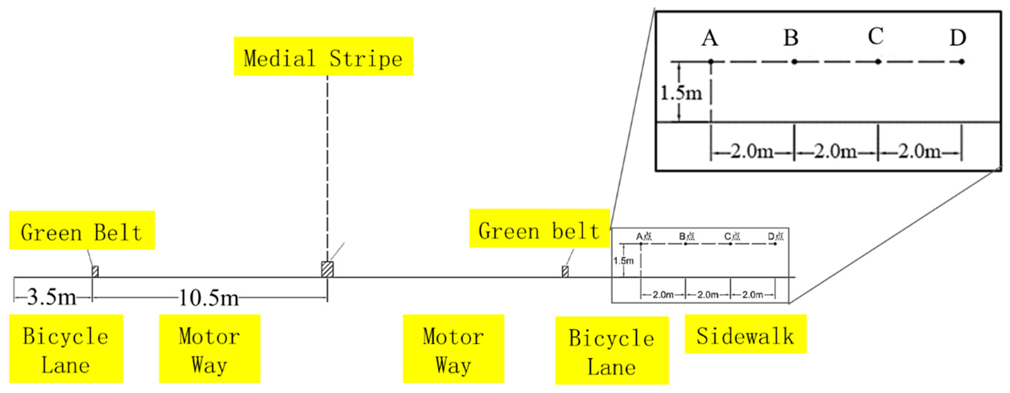
2.1. Field Measurement

Jinan city is located at 36°40′ N latitude and 116°57′ E longitude, northwest of Shandong Province, China [26]. Qingnian East Road, a traffic artery with typical road configuration (two-way, six-lane, double-sided sidewalk) located in the downtown area of Jinan city, was chosen as the representative trunk road for field monitoring. The observed road segment was between intersections to avoid the error caused by the concentration and dispersion of traffic flow and pedestrians. At the same time, the selected road section was flat, without vehicle climbing and turning errors and was not affected by side parking at bus stops or temporary stops. As such, the selected measurement segment was the road section between the cross-section of Qingnian East Road and Jingshi Road, and the cross-section of Qingnian East Road and Wenhua West Road. The monitoring location was selected at the midpoint of selected road segment, thus reducing the impact of vehicle stop and go, acceleration, deceleration, lane changing, and pedestrian crossing at intersections, etc. Situated in the city center of Jinan, the monitoring location is surrounded by some famous attractions, like Quancheng Park and Mount Qianfo, as well as urban functional areas like hospitals, universities, business district, and TV stations, and has a large traffic flow. Field measurements were conducted during PM peak hours in 20 April 2018, from 16:30 to 18:30, when the traffic flow was relatively steady in both volume and composition.

2.1.1. CO Concentration
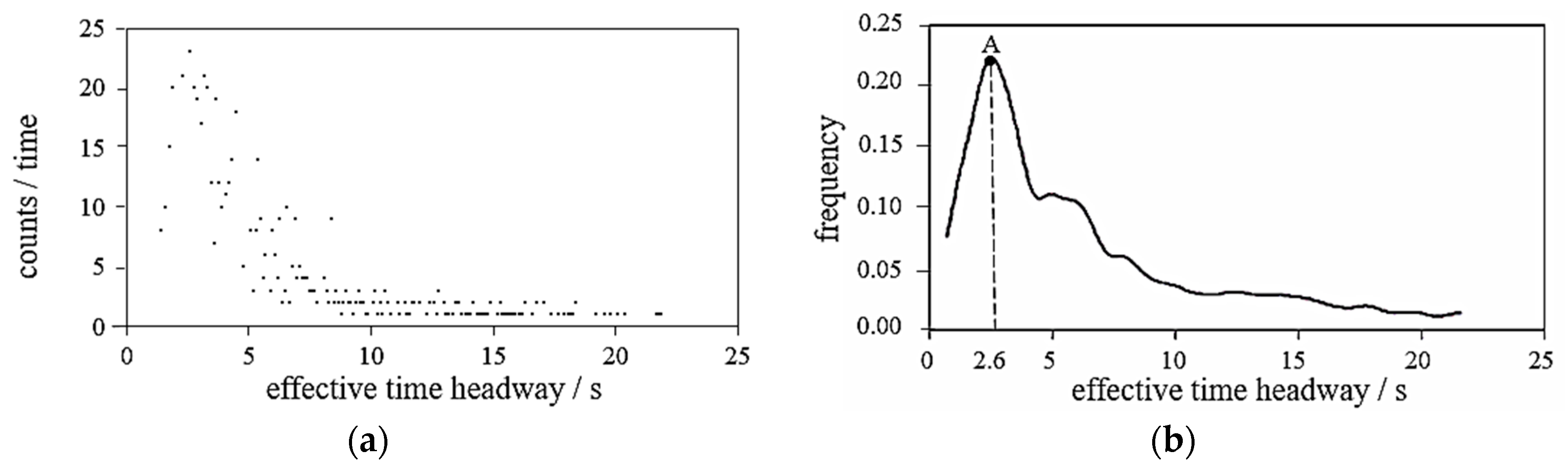
To provide real CO concentrations for examination, Langan Model T15n CO Measurers were used to collect and record CO concentrations for every 5 s. Four monitoring points (Figure 1) were perpendicular to the road direction from the roadside to the outside at pedestrian height (1.5 m). These points spanned 6-meter and are 2-meter apart from each other, to detect the variation of concentration, with comparable larger gradient in the perpendicular direction than along the road direction.
During the measurement, the temperature was about 26 °C, and the maximum and average wind speed were 2.5 m/s and 1 m/s, at the monitoring location, with the wind direction mainly coming from the north.

2.1.2. Traffic Flow

The average speed and space headway of the traffic flow during peak hours were captured by portable radar speed detectors and video recorders. In this paper, the Bushnell 10-1911 radar speedometer was adopted to collect the instantaneous velocity, and the recorded video was used to count the vehicles and calculate time headway manually. According to the dataset obtained, the representative peak hour was selected as 17:20–18:20. The peak hourly volume was 1080 vph (small passenger cars only), with an approximate average speed of 9.29 m/s. A total of 600 effective peak hour time headways were collected and the scatter diagram was plotted according to frequency counts in Figure 2a, where the X axis represents effective time headway and the Y axis represents counting times corresponding to the time headway reading from the recorded video. The probability distribution curve of the data was fitted in MATLAB (Figure 2b). The time headway (s) corresponding to the highest point (A) of the fitting curve was the saturated time headway, 2.6 s. With the average speed (9.29 m/s) calculated, the average space headway (m) of peak hour was approximated as 24.15 m using Equation (1) [27]
h s = V h t = 9.29 × 2.6 = 24.154 m .

2.2. Numerical Approach

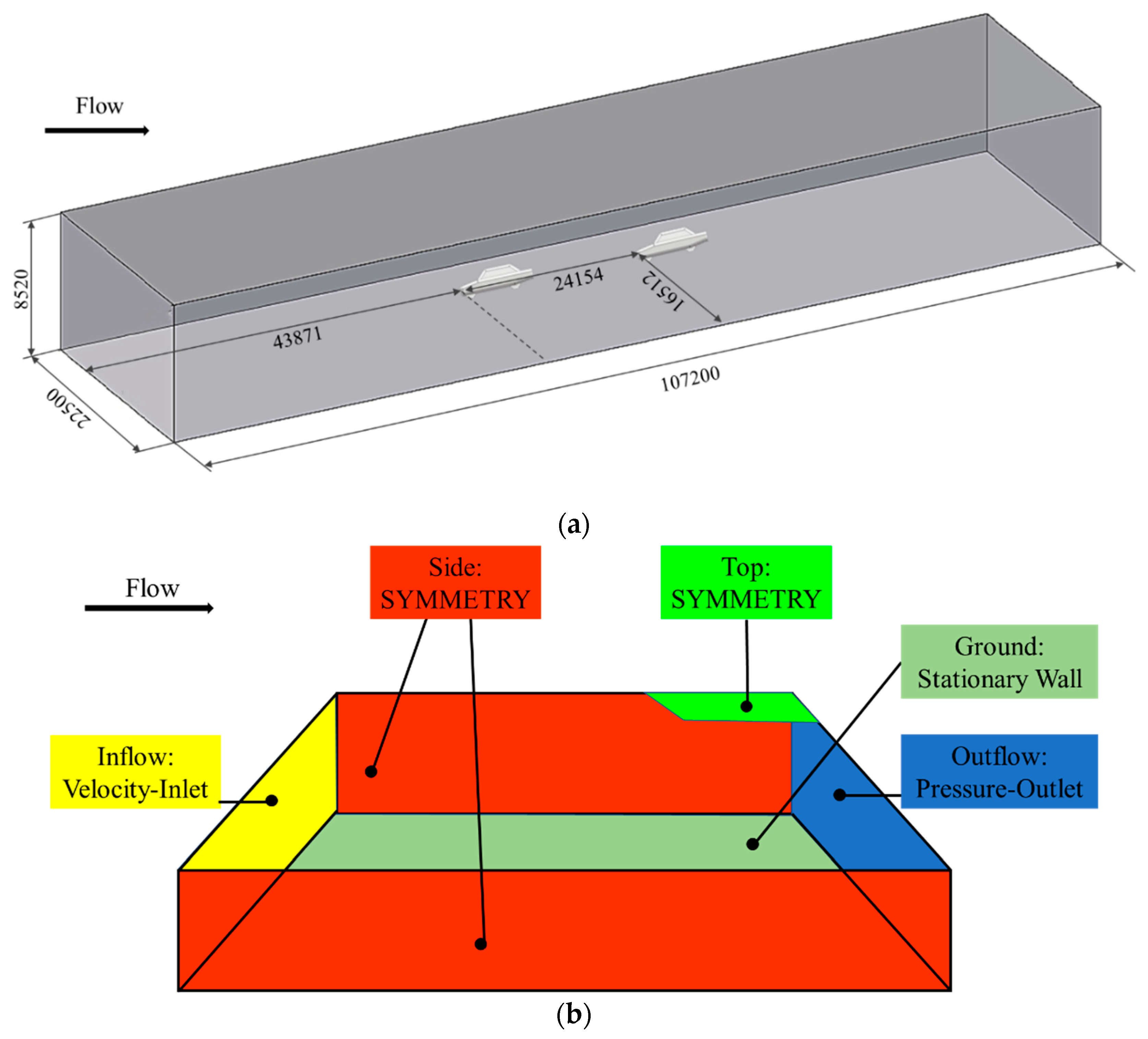
2.2.1. CFD Model Built-Up

A CFD simulation model including two vehicles on car-following state was established. According to the automobile sales statistics released by China Association of Automobile Manufacturers (CAAM) in 2017, the sales of sedans exceeded SUV and MPV, accounting for the highest market share [28]. Thus, the MIRA model of notch-back sedans was selected, as it has abundant aerodynamic resistance experimental data and the outline is similar to the actual vehicle surface streamline [29]. By setting the space headway as the average value of 24.15 m, the geometrical configuration of CFD numerical simulation was modeled and shown as in Figure 3a. The computational domain was established to be sufficiently large to imitate the actual flow field precisely, and the total blockage ratio was 0.968%, well below the 3% recommended criterion [30].

2.2.2. Mathematical Model

Because an automobile’s external flow field involves variations in traffic emission dispersion over time, and can be regarded as having unsteady, viscous, and incompressible flows [31], the governing equations in Cartesian coordinate system, as the derivation deduced by Batchelor et al. [32], includes continuity equations (Equation (2)) and momentum equations (Equation (3)):
ρ t + ( ρ u i ) x i = 0
( ρ u i ) t + ( ρ u i u j ) x j = p x i + τ i j x j + F i
τ i j = 2 μ S i j 2 3 μ u j x j δ i j
S i j = 1 2 ( u i x j + u j x i )
δ i j = { 0   ,   i j 1   ,   i = j
where ρ is the flow density, u i and u j are the component velocities in different directions, p is the flow pressure, F i is the component body force in one direction, t is time, x i , x j are coordinate components, τ i j is the viscous stress tensor (Equation (4)), μ is dynamic viscosity, S i j is the deformation rate tensor (Equation (5)), and δ i j is the Kerodiler function (Equation (6)), according to Blazek [33].
For the turbulence model, the RNG k ε model was used to calculate air flow process because it agrees with the experimental results and shows reliability in automobile flow field calculation problems [34,35]. In the light of Pulliam and Zingg [36], the turbulent kinetic energy k and the turbulence dissipation rate ε are set based on Equations (7) and (8), where R represents additional source term caused by deformation rate, μ t represents turbulence viscosity, as calculated by Equation (9)
( ρ k ) t + ρ u j k x j = x j [ ( μ + μ t σ k ) k x j ] + μ t u ¯ j x i ( u ¯ i x j + u ¯ j x i ) ρ ε
( ρ ε ) t + ρ u j ε x j = x j [ ( μ + μ t σ ε ) ε x j ] + c 1 ε k μ t u ¯ j x i ( u ¯ i x j + u ¯ j x i ) c 2 ρ ε 2 k R
μ t = c μ ρ k 2 ε .
u i ¯ and u j ¯ are the average of the transient values u i and u j . Turbulent Prandtl number for k and ε are represented by σ k and σ ε , respectively. Empirical constants c 1 , c 2 , and c μ have a given value of 1.44, 1.92, and 0.09, respectively.
Moreover, the emission dispersion process was calculated using special transport equations [37]:
( ρ μ Y i ) = ( ρ D i , e f f Y i ) + S i
D i , e f f = D i , m + μ t ρ S c t
where Y i is the mass fraction of component i, D i , e f f is the effective mass diffusion coefficient, D i , m is the molecular diffusivity, and S i is the generation rates. Meanwhile, S c t is the turbulent Schmidt number used to show the scalar dispersion competence of pollution, selected according to specific condition, with an optimal value ranging from 0.3 to 1.0 [38]. This study used a Schmidt number of 0.7.

2.2.3. CFD Parametrization

According to the wind speed, wind direction, and other information obtained from the field meteorological condition monitoring of the detecting location, corresponding computational domain boundary conditions (Figure 3b) can be set.
  • Inflow boundary: Velocity-Inlet, Temperature = 300 K, CO Mass Fraction = 0.001.
  • Outflow boundary: Pressure-Outlet, Static Pressure = 0.
  • Ground and vehicle body surface: Stationary Wall, Roughness Height (m) = 0, Roughness Constant = 0.5.
  • Top and side surfaces: SYMMETRY.
  • Exhaust pipe: Velocity-Inlet (VCO = 4.8 m/s), CO Mass Fraction = 0.1.
  • Flow (air): Pressure = 1.01325 × 10⁵ Pa, Temperature = 288 K, Density = 1.225 kg/m3, Dynamic Coefficient of Viscosity μ = 1.7894 × 10 5   Pa s , Kinematic Coefficient of Viscosity υ = μ / ρ = 1.461 × 10 5   m 2 / s .

2.2.4. CFD Model Assumptions

Focusing on simulating CO emission concentration distribution under car-following induced turbulence, some assumptions are used in this paper to achieve a balance between computational expense and simulation precision.
Assumption 1.
The automobile external flow field can be regarded as unsteady, viscous, and incompressible flow, which is consistent with the continuous medium hypothesis for establishing the N-S equation of fluid dynamics.
Assumption 2.
The model treats the motor vehicle as a closed entity and neglects the exchange of internal and external fields caused by the opening of the skylight, side window, or external circulation system of the vehicle. Therefore, the steering wheel, seats, and other interior parts of the vehicle are ignored.
Assumption 3.
The influence of vehicle surface details and slight deformation on the flow field outside the vehicle is ignored. Therefore, the CFD vehicle model is only built with the external frame structure of the specified vehicle, while the mirrors, bumpers, grille, sealing element, handrail, and external antenna are ignored.
Assumption 4.
Based on the demand of tail gas emission simulation, the motor vehicle exhaust pipe does not belong to the detailed components in Assumption 3 and should be simulated separately.
Assumption 5.
Compared to dynamic impacts of emission flow, the thermal effects are considered to be less significant.
Assumption 6.
Under actual road conditions, traffic flow is fluctuating all the time. However, given the limitations of computer processing power and the complexity of fluctuant traffic flow simulation, it is almost impossible to fully simulate traffic flow changes. Thus, the vehicles in the simulation model are moving forward at the same speed. And the more complicated fluctuant traffic flow situation can be simulated further on the basis of this study.

2.3. Grid Sensitivity Analysis

Unstructured grid was adopted around the vehicle, and structural grid was adopted in the computational domain periphery. In addition, the vehicle surface, ground area, and trailing vortex area were divided into detailed mixed grid schemes. To ensure that the simulation result data were independent from the grid resolution, a grid sensitivity analysis was carried before starting the calculation, since grid size can influence error propagating (13). The precision of grid size was divided into four scales: Low, Medium-low, Normal, and High, corresponding to maximum grid size of 0.25 m, 0.3 m, 0.35 m, and 0.4 m, separately, in ANSYS ICEM CFD software. Testing the four precision scales, with aerodynamic resistance coefficient ( C d ) as the inspection standard:
C d = F / ( q S )
where F is the aerodynamic resistance, q is the inflow dynamic pressures, and S is the frontal projected area of vehicle. Selecting the CODASC wind tunnel experiments data 0.3055 as the standard C d [39], a residual convergence of 10−5 was used for four cases. The grid quantity and C d results are summarized in Table 1.
As shown in Table 1, when the maximum grid size is 0.4 m and 0.35 m, the number of grids was small and the simulation accuracy was poor. When the maximum grid size was 0.3 m and 0.25 m, errors of both were less than 5% of the previous result, but the difference of grid number was nearly doubled, indicating that when the maximum size was less than 0.3 m, further refinement of grid had little effect on improving computational accuracy. Therefore, the Normal precision was adopted to divide the formal computational domain grid. This divide scheme not only achieved grid independence, but also obtained a balance between accuracy and CPU time.

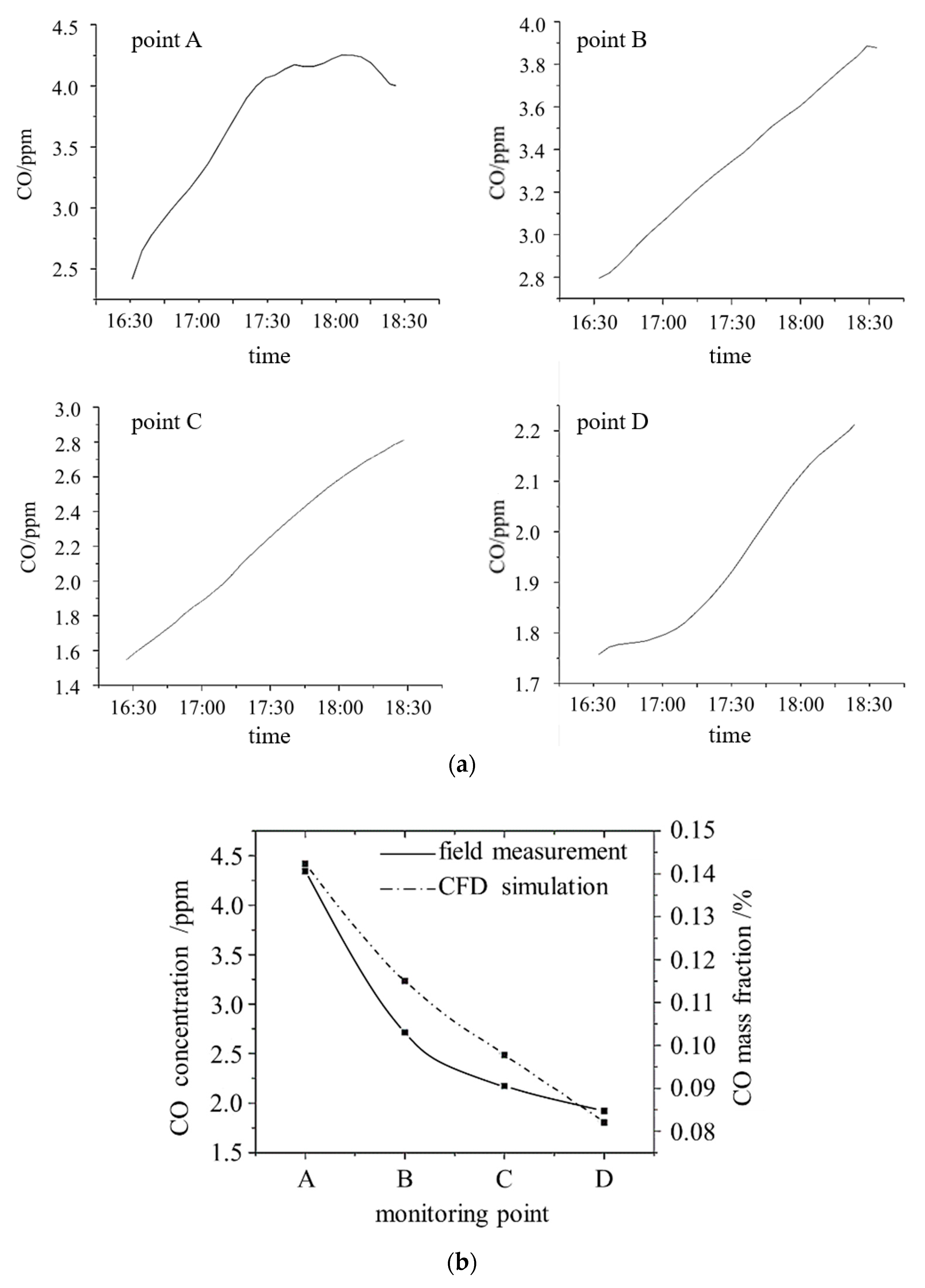
2.4. Model Calibration

The CFD simulated CO mass fraction was further verified with the field measurements. Due to the low concentration of CO in the air, the measurers may suffer with readings deviation. As a result, the CO concentration obtained from sampling was averaged before comparison (Figure 4a).
The overall measured roadside CO concentration presented a steady rise trend, and the reasons were preliminarily speculated as follows:
  • The monitoring duration was at the evening peak, with large motor vehicle flow and high CO emission intensity;
  • There are tall buildings on both sides of the monitoring locations, and CO was easy to accumulate there;
  • On the day of experiment, the wind speed was small, which makes it difficult for CO to enter the surrounding area.
After the simulation converged, comparison between the simulation output and the averaged measurements were plotted in Figure 4b. The dotted line represents the CO mass fraction obtained by numerical simulation, while the solid line is the CO concentration obtained by field monitoring.
To ensure the effectiveness of the simulation, the monitoring points were set perpendicular to the road. If the simulation was inaccurate, the output curve would largely deviate from the observed value. In Figure 4b, the overall trend of simulation curve was in accordance with the field measurement curve. Moreover, the percentage uncertainty of CFD simulation compared to the field measurement at four monitoring points (A, B, C, D, see Figure 1) was 2.3%, 18.2%, 14.5%, and 6.2%, respectively, all far lower than the results from the previous study, which is about 30% [40]. Therefore, the simulation model and outputs were recognized as valid.
In addition to a validation between the data obtained with CFD and the field measurement, other previous literature were examined to assure simulation accuracy. The pressure coefficients of the front-vehicle surface are plotted in Figure 5. The pressure on the front of the car and the window was high, and there was a negative pressure area at the junction of the window and the upper surface of the car body. The pressure coefficient distribution and the value of pressure were consistent with the previous studies [41,42,43]. Thus, the robustness of the model is verified.

3. Results and Discussion

To further investigate the spatial and temporal flow pattern of traffic exhaust, steady-state simulations and transient simulations were performed. The main results are as follows.

3.1. Steady-State Simulation Results

3.1.1. Verification of Existence of VIT Influence

To verify that vehicle induced turbulence influence the flow pattern of on-road emission, velocity vector of the front- and rear-vehicles surrounding in the exhaust pipe longitudinal section are shown in Figure 6a. Through the spatial distribution of velocity vector, difference of exhaust flow pattern, related closely to air motion, can be performed. Here the velocity of the inflow boundary was set to 10.29 m/s, equaling to the fleet average speed plus the opposite average wind speed from north in peak hours, i.e., the speed of the wind relative to the car.
As can be seen from Figure 6a, the blocking effect of vehicles on the flow field makes the airflow velocity in the head, windshield, and tail of vehicles decrease significantly. Moreover, when vehicles are in the normally car-following situations, the air velocity around the two vehicles is obviously different, and the velocity around the rear car is generally lower. The blocking effect of front car causes the airflow to converge at the tail, forming a complex trailing vortex area, where vortexes are constantly generated, rotated, and shed, resulting in the energy loss of airflow impinging on the rear car. Thus, airflow velocity at the head of rear car is remarkably lower than that of the front car. At the same time, the blocking effect of rear car induces boundary layer and turbulent separation area around the rear vehicle, aggravating the velocity decrease at the windshield, the interface of the windshield, the and car roof and underbody, compared to the front vehicle. Due to a distinct difference existing in the velocity vector around both front- and rear-vehicles, emission diffusion is bound to be different, indicating that vehicle induced turbulence has an impact on the on-road emission flow pattern. To explore the specific influence of vehicle induced turbulence on the flow pattern of traffic exhaust, the characteristics of the flow field both perpendicular to and along the road direction were analyzed separately.

3.1.2. Influence of VIT in Direction along the Road

In the direction along the road, the CO mass fraction distribution map in the exhaust pipe longitudinal section is shown in Figure 6b. A red color indicates the highest CO concentration, followed by green, while blue indicates the lower concentration, and white indicates the lowest. It can be observed that the flow pattern of vehicle pollutant near the exhaust pipe remains consistent, but the emission of rear car diffuses faster. The concentration distribution map with CO mass fraction of 0.0012 is presented in Figure 6c. By comparing the dark blue areas with same CO mass fraction (=0.0012) along the tail of the two vehicles, it can be figured out that the dark blue area of the rear car has an extension distance (12.7 m) about twice as large as that of the front car (6.0 m). The trailing vortex area caused by the front car as well as the external surface boundary layer and turbulent separation area caused by the rear car impede the emission diffusion of front car and reduce diffusion dilution speed. As shown in Figure 6a, the interval from the tail of front car to the head of rear car is a low-speed flow area, indicating that VIT hinders the emission diffusion of the front car by reducing the airflow velocity.

3.1.3. Influence of VIT in Direction Perpendicular to the Road

In the direction perpendicular to the road, Figure 6d shows the partially enlarged CO mass fraction map of a cross section at 4 m behind the tail of the front car, 4 m behind the tail of the rear car and 6 times vehicle length behind the tail of the rear car, respectively. Through comparison, on-road emissions of the rear car diffuse faster than that of the front car at the same distance (4 m) behind the two vehicle tails in direction perpendicular to the road. The equal-scale enlargement map of Figure 6d indicates the existence of a large concentration gradient area in the cross section. In fact, the large concentration gradient area is within a range of 1 m on both sides of the vehicle’s body, even in the well-diffused cross section which is 6 times the vehicle length behind the tail of the rear car. The CO mass fraction at the exhaust pipe is 0.1, and the ambient background CO concentration is 0.001. Thus, the total concentration gradient is 0.999. However, the mass fraction at 1 m away from the vehicle body decreased to 1.15 × 10⁻³, so there was a large concentration gradient area accounting for 99.85% of the total concentration gradient only within 1 m on both sides of the vehicle’s body.
To determine the specific numerical relationship between on-road emission concentration and background emission concentration 1 m away from vehicle sides, quantitative analysis was carried out on the concentration of two intersected lines which are parallel to and 1 m apart from the left and right vehicle sides, at the pedestrian breathing height (1.5 m) level, as shown in Figure 6e. It can be inferred that the right side concentration curve first increases compared with the left side, and the on-road emissions reached the right intersected line fast. Moreover, at the same distance behind the exhaust pipe of the front car, the emission concentration of the right intersected line (solid line) was higher than that of the left (dash line). This is mainly because the exhaust pipe is on the right side of vehicle center longitudinal section, so that the right intersected line is closer to the exhaust pipe.
In terms of pollutant concentration, the difference between the numerical value of the two curves in Figure 6e and the background concentration (0.001) was less than 10−6, and concentration at vehicle side 1 m was very close to the background concentration. Namely, the effect of vehicle induced turbulence caused by front- and rear-vehicles on the traffic exhaust flow pattern was limited. More importantly, within a range of 1 m on both sides of the vehicle body there was a rather large concentration gradient area, containing sharp mechanical turbulence and a complex on-road emission flow mechanism. In this region, VIT should be considered carefully as it could have a dominant influence on the emissions concentration.

3.2. Transient Simulation Results

In addition to the steady-state simulation, the transient simulation assists to obtain the process of physical quantity changing with time. Different from most previous correlated studies, to make the numerical simulation more accurate, this paper used dynamic grid technology to solve the fluid boundary motion problem in a transient simulation, which can better simulate the shape of flow field changing with time due to boundary motion. A layering grid update method in the ANSYS Fluent software was applied to establish the dynamic grid model. The motion state of vehicles in the CFD model built in Section 2.2.1 can be defined using transient profiles, which use time and speed of point seriation to specify the motion mode of the component [44]. Here the vehicle speed was set to 9.29 m/s, and velocity of the inflow boundary was set to 1 m/s as the average wind velocity. Two vehicles were assumed to move at the same speed in 4 s together in the computing domain. The single simulation time step was set at 0.005 s, and the total simulation time steps were 800.

3.2.1. Judgment of Stable Driving State

It is necessary to get time steps in order to reach the stable moving state. Different from the continuous running situation on real roads, in the early stage of simulation, two vehicle models started from being static. Therefore, the initial simulative stage should be eliminated during the analysis process. The aerodynamic resistance coefficient C d was used to determine whether the vehicle had reached a stable driving state. When C d was stable at a certain value, the state was considered as stable. Upon taking 0.1 s (20 steps) as the time interval for statistical analysis, C d was basically stable at 0.3 after 200 steps. Therefore, the analysis was based on the time step larger than 200 (time after 1 s).

3.2.2. Influence of VIT over Time

Figure 7 presents the corresponding relationship between the vehicle position and the velocity field. The reference plane was selected at the cross Section 4 m behind the tail of the front vehicle at the beginning of the simulation. The observation interval was 0.6 s. For the process of the rear car approaching, passing, and leaving the reference plane, the high-speed diffusion area focused on a small portion of the field, since large areas of the periphery had a low air flow velocity. It could be inferred that the low emission concentration at 1 m away from the vehicle sides was affected by the low airflow velocity. Meanwhile, when the rear car left the reference plane, the velocity map of the reference plane had no obvious changes since the tail of the rear car was 9 m away from the plane. In this case (9.29 m/s speed, 24.15 m space headway), 9 m behind the rear car was recognized as the airflow disturbance zone, with the influence of VIT weakening after 9 m.

4. Conclusions

In this paper, a CFD numerical simulation of on-road emission flow pattern in urban roads was performed to verify and reveal the influence of vehicle induced turbulence. A complex fleet situation was decomposed into the superposition of front- and rear-car following models, and the influence of VIT on one group of car-following models was studied. Conclusions can be drawn as follows:
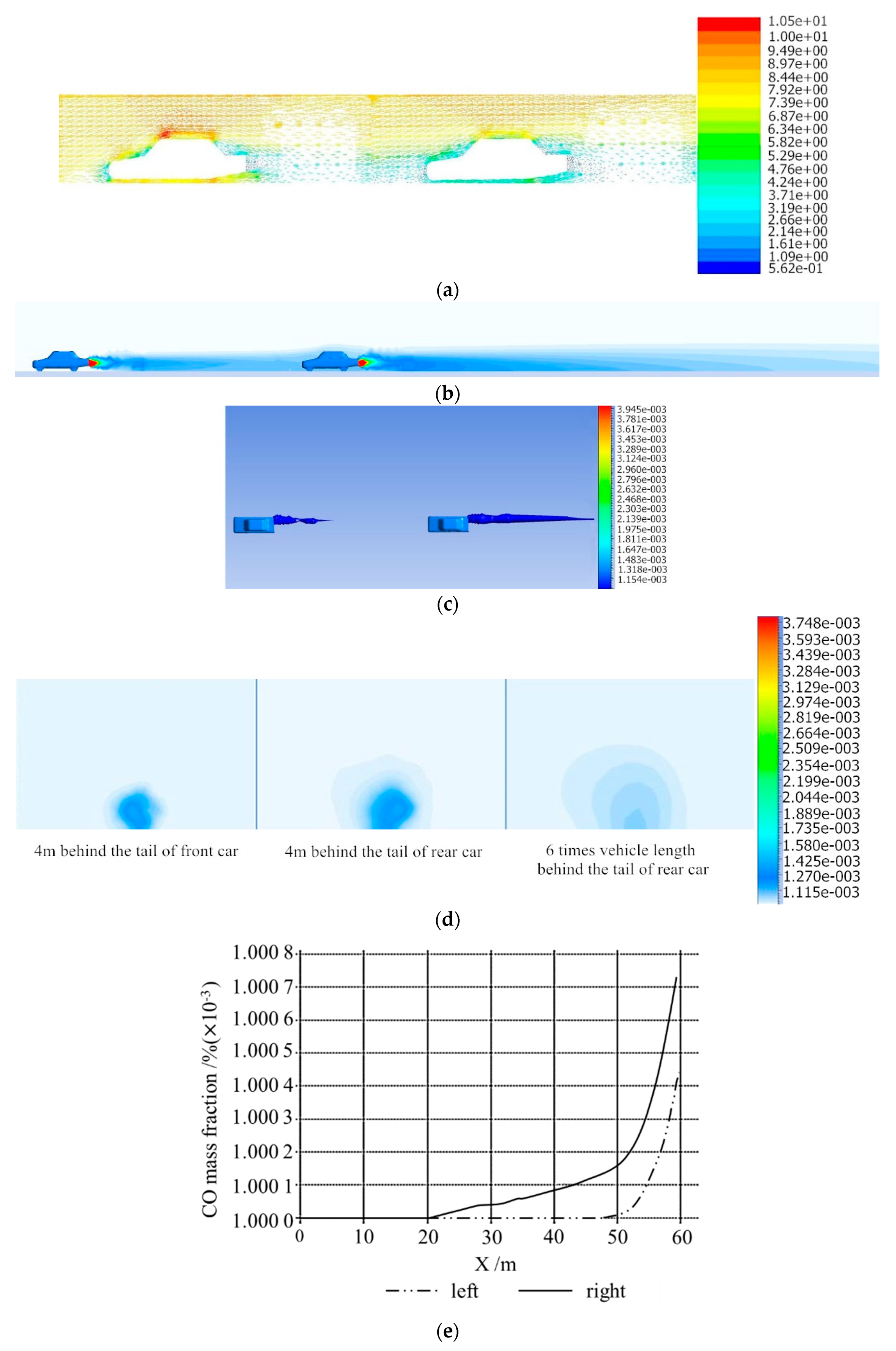
  • The vehicle induced turbulence caused by front- and rear-vehicles impedes the diffusion of traffic exhaust of the front car. Until the convergence timing occurred in the steady simulation, the front-vehicle isosurface with the CO mass fraction of 0.0012 extended to 6.0 m behind the vehicle, while rear-vehicle isosurface with the CO mass fraction of 0.0012 extended to 12.7 m behind the vehicle. Thus, in the direction along the road, the dispersion speed of the rear car pollutant was about twice that of the front one. According to Wang et al. [45], the CO concentration of a single car drops to a number near the background concentration within 4 m of the vehicle rear, which is lower than the results in this paper. By comparison, we can draw the conclusion that although the emissions of the front vehicle disperse slower than that of the rear vehicle, from an overall perspective, VIT is beneficial to the diffusion of pollutants of a motorcade.
  • In the direction perpendicular to the road, the VIT influence area is generally concentrated within 1 m of the vehicle side. This result is consistent with the research of Wang et al. [45], which concluded that the concentration is relatively high within the radius of the exhaust pipe from 1 m to 1.5 m. That is, within a range of 1 m on both sides of vehicle there is a large concentration gradient area, which accounts for 99.85% of the total concentration gradient between the background environment and the exhaust pipe, which contains sharp mechanical turbulence and a complex traffic exhaust flow mechanism. In the large concentration gradient region, VIT should be considered carefully since it might affect the on-road emissions concentration.
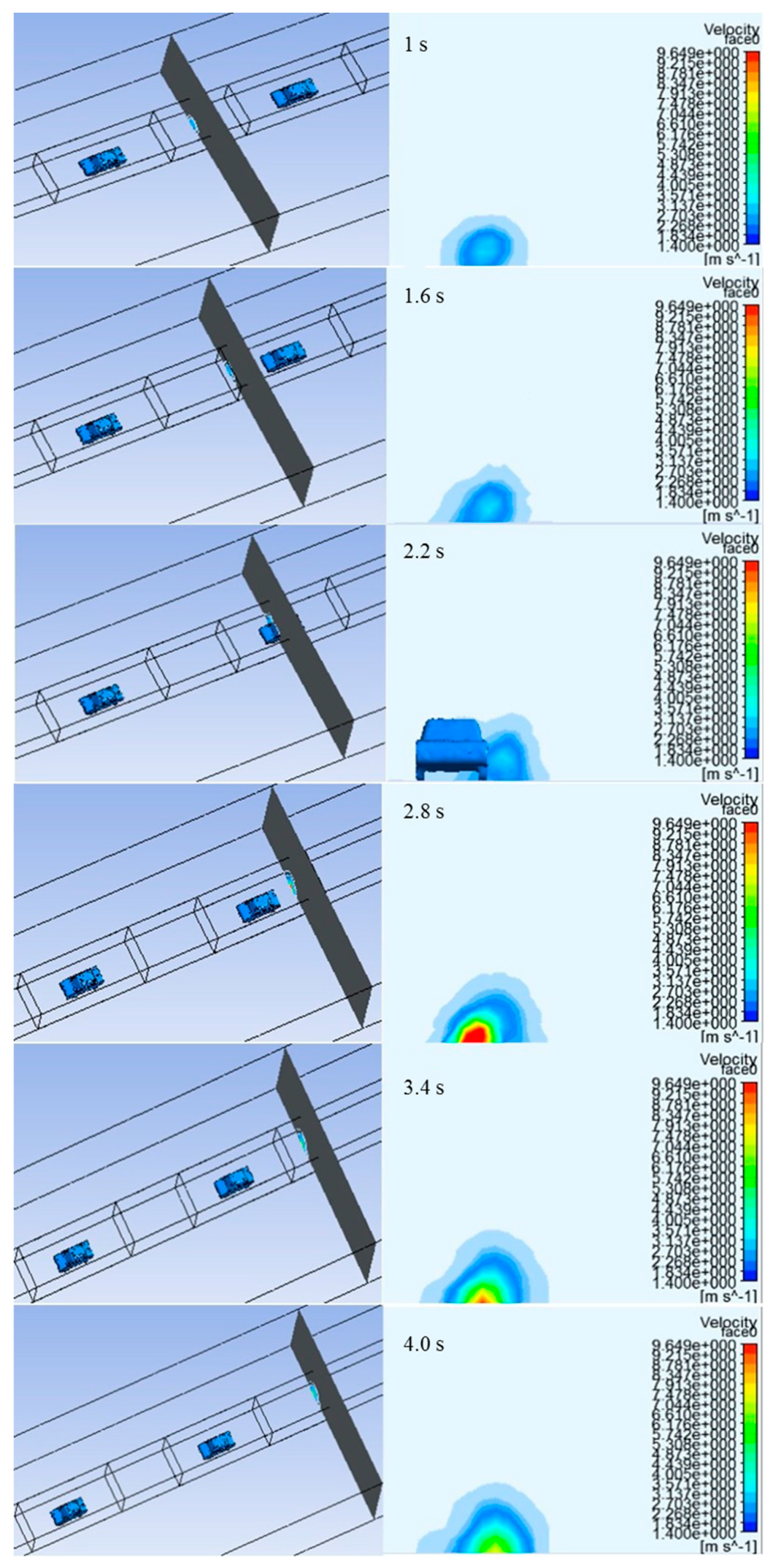
  • In this research, with the fleet average speed of 9.29 m/s and the average space headway of 24.15 m, the vehicle induced turbulence zone was approximated within a range of 9 m behind the rear car, afterwards the influence of VIT weakened.
The main limitation of the CFD simulation model proposed in this paper is that the fluctuant traffic flow was simplified into vehicle fleet of uniform motion, due to the assumptions imposed in Section 2.2.4. In addition, only the MIRA model of notch-back sedans was selected to explore the emissions flow pattern in this paper based on the statistics of actual road vehicle composition. However, the model calibration introduced in Section 2.4 concludes that the assumptions applied can simulate the actual condition well.
Overall, this paper supplemented research on vehicle pollutant flow pattern regularity and paved the way for using CFD to investigate the influence of vehicle induced turbulence. The outcomes discovered in this study have practical significance, which assists to minimize the adverse impacts of heavy vehicle emissions through reasonable traffic management and planning. For example, relieving traffic congestion and making sure that vehicles in a car fleet have a large space headway can effectively speed up vehicle pollutant diffusion, as exhaust dispersion of the front car can be impeded on by the rear-vehicle airflow blocking effect. Moreover, it is recommended to set a green belt or other infrastructure to keep a distance between the outside lane and adjacent non-motorized lane that is greater than 1 m, to avoid the risk of riders in the non-motorized lane and pedestrians inhaling excessive automobile exhaust.
Results in this paper suggested the application scope of the line source traffic emission model, which may be utilized in emission quantitative statistics and studies about roadside traffic pollution distribution. However, when using a complex turbulent flow field for surrounding the vehicle, involving the influence of road barriers and a green belt on traffic exhaust diffusion and so on, simplified line source models may induce remarkable errors at a 10−1 order of magnitude. Future research can focus on supplementing the vehicle model and the improvement of real traffic flow fluctuant imitation in simulations. Other vehicle models, such as trucks, or combinations of vehicle models can be used to explore the differences between VIT impacts on various motorcycle types. Moreover, a dynamic motorcade model which considers the distribution frequency of the vehicle speed may be established to improve simulation accuracy and better reflect actual vehicle movement. Further studies may be conducted to reveal the specific manifestation of the concentration differences between line source models and the actual situations by incorporating dense monitoring data, refined models, and even large amounts of big data [46].

Author Contributions

Study conception and design: X.S. and D.S.; Data collection: X.S. and S.F.; Analysis and interpretation of results: Z.Z. and J.L.; Draft manuscript preparation: X.S., D.S. and J.L.

Funding

The research was funded in part by the National Nature Science Foundation of China [71971138], and the Humanities and Social Science Research Project, Ministry of Education, China [18YJCZH011, 19YJAZH077], and the Shanghai “Science and Technology Innovation Action Plan”—“One Belt and One Road” International Cooperation Project [19210745600]. Any opinions, findings and conclusions or recommendations expressed in this paper are those of the authors and do not necessarily reflect the views of the sponsors.

Acknowledgments

The authors would express their appreciation to Taha Benarbia, Institution of Maintenance and Industrial Security (IMIS), University of Oran, Algeria, for his valuable suggestions and assistance in this study.

Conflicts of Interest

The authors declare no conflict of interest.

References

  1. Hao, H.; Wang, H.; Yi, R. Hybrid Modeling of China’s Vehicle Ownership and Projection through 2050. Energy 2011, 36, 1351–1361. [Google Scholar] [CrossRef]
  2. Zhang, L.; Long, R.; Chen, H.; Geng, J. A Review of China’s Road Traffic Carbon Emissions. J. Clean. Prod. 2019, 207, 569–581. [Google Scholar] [CrossRef]
  3. Barnes, J.H.; Chatterton, T.J.; Longhurst, J.W.S. Emissions vs Exposure: Increasing Injustice from Road Traffic-related Air Pollution in the United Kingdom. Transp. Res. Part D Transp. Environ. 2019, 73, 56–66. [Google Scholar] [CrossRef]
  4. Vardoulakis, S.; Fisher, B.E.A.; Pericleous, K.; Gonzalez-Flesca, N. Modelling Air Quality in Street Canyons: A Review. Atmos. Environ. 2003, 37, 155–182. [Google Scholar] [CrossRef]
  5. Jones, S.G.; Fisher, B.E.A.; Gonzalez–Flesca, N.; Sokhi, R. The Use of Measurement Programmes and Models to Assess Concentrations next to Major Roads in Urban Areas. Environ. Monit. Assess. 2000, 64, 531–547. [Google Scholar] [CrossRef]
  6. Hertel, O.; Berkowicz, R. Modelling Pollution from Traffic in a Street Canyon. Evaluation of Data and Model Development; NERI: Roskilde, Denmark, 1989. [Google Scholar]
  7. Gosman, A.D. Developments in CFD for Industrial and Environmental Applications in Wind Engineering. J. Wind Eng. Ind. Aerodyn. 1999, 81, 21–39. [Google Scholar] [CrossRef]
  8. Kondo, H.; Tomizuka, T. A numerical Experiment of Roadside Diffusion under Traffic-produced Flow and Turbulence. Atmos. Environ. 2009, 43, 4137–4147. [Google Scholar] [CrossRef]
  9. Parra, M.A.; Santiago, J.L.; Martin, F.; Martilli, A.; Santamaria, J.M. A Methodology to Urban Air Quality Assessment during Large Time Periods of Winter using Computational Fluid Dynamic Models. Atmos. Environ. 2010, 44, 2089–2097. [Google Scholar] [CrossRef]
  10. Wang, L.; Jayaratne, R.; Heuff, D.; Morawska, L. Development of a Composite Line Source Emission Model for Traffic Interrupted Microenvironments and its Application in Particle Number Emissions at a Bus Station. Atmos. Environ. 2010, 44, 3269–3277. [Google Scholar] [CrossRef]
  11. Sun, D.J.; Zhang, K.S.; Shen, S.W. Analyzing Spatiotemporal Traffic Line Source Emissions based on Massive Didi Online car-hailing Service Data. Transp. Res. Part D Transp. Environ. 2018, 62, 699–714. [Google Scholar] [CrossRef]
  12. Ming, T.Z.; Fang, W.J.; Peng, C.; Cai, C.J.; De Richter, R.; Ahmadi, M.H.; Wen, Y.G. Impacts of Traffic Tidal Flow on Pollutant Dispersion in a Non-Uniform Urban Street Canyon. Atmosphere 2018, 9, 82. [Google Scholar] [CrossRef]
  13. Jeanjean, A.P.R.; Hinchliffe, G.; McMulla, W.A.; Monks, P.S.; Leigh, R.J. A CFD study on the effectiveness of trees to disperse road traffic emissions at a city scale. Atmos. Environ. 2015, 120, 1–14. [Google Scholar] [CrossRef]
  14. Sun, D.J.; Zhang, Y. Influence of Avenue Trees on Traffic Pollutant Dispersion in Asymmetric Street Canyons: Numerical Modelling with Empirical Analysis. Transp. Res. Part D Transp. Environ. 2018, 65, 784–795. [Google Scholar] [CrossRef]
  15. Buccolieri, R.; Gromke, C.; Sabatino, S.D.; Ruck, B. Aerodynamic Effects of Trees on Pollutant Concentration in Street Canyons. Sci. Total Environ. 2009, 407, 5247–5256. [Google Scholar] [CrossRef] [PubMed]
  16. Meroney, R.N.; Pavageau, M.; Rafailidis, S.; Schatzmann, M. Study of Line Source Characteristics for 2–D Physical Modelling of Pollutant Dispersion in Street Canyons. J. Wind Eng. Ind. Aerodyn. 1996, 62, 37–56. [Google Scholar] [CrossRef]
  17. Sanchez, B.; Santiago, J.L.; Martilli, A.; Martin, F.; Borge, R.; Quaassdorff, C.; de la Paz, D. Modelling NOx Concentrations through CFD–RANS in an Urban Hot-spot using High Resolution Traffic Emissions and Meteorology from a Mesoscale Model. Atmos. Environ. 2017, 163, 155–165. [Google Scholar] [CrossRef]
  18. Hucho, W.H.; Sovran, G. Aerodynamics of Road Vehicles. Annu. Rev. Fluid Mech. 1993, 25, 485–537. [Google Scholar] [CrossRef]
  19. Rao, S.T.; Sedefian, L.; Czapski, U.H. Characteristics of Turbulence and Dispersion of Pollutants near Major Highways. J. Appl. Meteorol. Climatol. 1979, 18, 283–293. [Google Scholar]
  20. Kastner–Klein, P.; Berkowicz, R.; Plate, E.J. Modelling of Vehicle-induced Turbulence in Air Pollution Studies for Streets. Int. J. Environ. Pollut. 2000, 14, 496–507. [Google Scholar] [CrossRef]
  21. Deng, S.X.; Guan, Y.L. Analytical Solutions of Atmospheric Diffusion Equation with Multi Sources from Roads. J. Changan UNIV 2005, 25, 94–99. [Google Scholar]
  22. Zhang, K.M.; Wexler, A.S.; Niemeier, A.S.; Zhu, Y.F.; Hinds, W.C.; Sioutas, C. Evolution of Particle Number Distribution near Roadways. Part III: Traffic Analysis and On-road Size Resolved Particulate Emission Factors. Atmos. Environ. 2005, 39, 4155–4166. [Google Scholar] [CrossRef]
  23. Zou, Y.; Zhao, X.; Chen, Q. Comparison of STAR-CCM+ and ANSYS Fluent for Simulating Indoor Airflows. Build. Simul. 2018, 11, 165–174. [Google Scholar] [CrossRef]
  24. Greifzu, F.; Kratzsch, C.; Forgber, T.; Lindener, F.; Schwarze, R. Assessment of Particle-tracking Models for Dispersed Particle-laden Flows Implemented in OpenFOAM and ANSYS FLUENT. Eng. Appl. Comput. Fluid Mech. 2016, 10, 30–43. [Google Scholar] [CrossRef]
  25. Versteeg, H.K.; Malalasekera, W. An Introduction to Computational Fluid Dynamics: The Finite Volume Method, 2nd ed.; Pearson Prentice Hall: New York, NY, USA, 2007. [Google Scholar]
  26. Liu, W.J.; Jiao, F.C.; Ren, L.J.; Xu, X.G.; Wang, J.C.; Wang, X. Coupling Coordination Relationship between Urbanization and Atmospheric Environment Security in Jinan City. J. Clean. Prod. 2018, 204, 1–11. [Google Scholar] [CrossRef]
  27. Fricker, J.D.; Whitford, R.K. Fundamentals of Transportation Engineering: A Multimodal Systems Approach; Pearson Prentice Hall: Upper Saddle River, USA, 2007. [Google Scholar]
  28. The Top Ten Passenger Car Brands in 2017. Available online: http://www.caam.org.cn/chn/4/cate_31/con_5214783.html (accessed on 10 November 2018).
  29. Le Good, G.M.; Garry, K.P. On the Use of Reference Models in Automotive Aerodynamics. In Proceedings of the 2004 SAE World Congress and Exhibition, Detroit, MI, USA, 8–11 March 2004. [Google Scholar]
  30. Franke, J.; Hellsten, A.; Schlunzen, K.H.; Carissimo, B. The COST 732 Best Practice Guideline for CFD Simulation of Flows in the Urban Environment: A Summary. Int. J. Environ. Pollut. 2011, 44, 419–427. [Google Scholar] [CrossRef]
  31. Li, L.; Du, G.S.; Liu, Z.G.; Lei, L. The Transient Aerodynamic Characteristics around Vans Running into a Road Tunnel. J. Hydrodyn. 2010, 22, 283–288. [Google Scholar] [CrossRef]
  32. Batchelor, G.K. Equations Governing the Motion of a Fluid, in: An Introduction to Fluid Dynamics; Cambridge University Press: Cambridge, UK, 2000. [Google Scholar]
  33. Blazek, J. Computational Fluid Dynamics: Principles and Applications, 2nd ed.; Elsevier, Ltd.: Amsterdam, The Netherlands, 2005. [Google Scholar]
  34. Zhang, M.L.; Shen, Y.M. Three-dimensional Simulation of Meandering River based on 3D RNG Turbulence model. J. Hydrodyn. 2008, 20, 448–455. [Google Scholar] [CrossRef]
  35. Chen, X.; Lu, C.J.; Li, J.; Pan, Z.C. The Wall Effect on Ventilated Cavitating Flows in Closed Cavitation Tunnels. J. Hydrodyn. 2008, 20, 561–566. [Google Scholar] [CrossRef]
  36. Pulliam, T.H.; Zingg, D.W. Fundamentals of Computational Fluid Dynamics; Springer: Berlin, Germany, 2001. [Google Scholar]
  37. Mika, S.; Brandner, M. Numerical Modelling of Some Two-phase Fluid Flow Problems. Math. Comput. Simul. 2004, 67, 301–305. [Google Scholar] [CrossRef]
  38. Vranckx, S.; Vos, P.; Maiheu, B.; Janssen, S. Impact of Trees on Pollutant Dispersion in Street Canyons: A Numerical Study of the Annual Average Effects in Antwerp, Belgium. Sci. Total Environ. 2015, 532, 474–483. [Google Scholar] [CrossRef]
  39. Concentration Data of Street Canyon. Laboratory of Building and Environ-mental Aerodynamics. Available online: http://www.ifh.uni-karlsruhe.de/science/aerodyn/CODASC.htm (accessed on 27 November 2018).
  40. Openfoam CFD Simulation of Pollutant Dispersion in Street Canyons: Validation and Annual Impact of Trees. Available online: http://www.irceline.be/atmosys/faces/doc/ATMOSYS_Deliverable_9.2b_windtunnel%20validation.pdf (accessed on 27 November 2018).
  41. Himeno, R.; Fujitani, K. Numerical analysis and visualization of flow in automobile aerodynamics development. J. Wind Eng. Ind. Aerodyn. 1993, 785–790. [Google Scholar] [CrossRef]
  42. Wang, J.Z. Numerical Simulation of Vehicle Pollutant Dispersion in Urban Street Canyon; Shandong UNIV: Jinan, China, 2012. [Google Scholar]
  43. Tsubokura, M.; Yamada, N.; Kitayama, S. Effects of Body Shapes on Unsteady Aerodynamics of Road Vehicles in a Gusty Crosswind. In Proceedings of the 28th AIAA Applied Aerodynamics Conference, Chicago, IL, USA, 28 June–1 July 2010. [Google Scholar]
  44. Fluent Inc. Fluent User’s Guide; Version 5.0; Fluent Inc.: Lebanon, NH, USA, 1998. [Google Scholar]
  45. Wang, J.S.; Chan, T.L.; Huang, Z.; Cheung, C.S.; Ning, Z. The prediction and field observation for Pollutant Dispersion from Vehicular Exhaust Plume in Real Atmospheric Environment. J. Shanghai Jiaotong Univ. 2005, 39, 1891–1894. [Google Scholar]
  46. Sun, D.S.; Ding, X. Spatiotemporal evolution of ridesourcing markets under the new restriction policy: A case study in Shanghai. Transp. Res. Part A Policy Pract. 2019, 130, 227–239. [Google Scholar] [CrossRef]
Figure 1. Arrangement of the monitoring points on the field measurement position.
Sustainability 11 06705 g001
Figure 2. Obtained saturated headway from 600 effective headways measured, (a) Counts–effective time headway scatter diagram, (b) Probability distribution curve.
Sustainability 11 06705 g002
Figure 3. Computational domain diagram, (a) Simulation model (unit: mm), (b) Boundary conditions used for the simulation.
Sustainability 11 06705 g003
Figure 4. Road side carbon monoxide (CO) concentration curve, (a) Averaged monitoring concentration curve of A, B, C, and D points, (b) Comparison of CO concentration between simulation and field measurement.
Sustainability 11 06705 g004
Figure 5. Pressure coefficient diagram of front car surface.
Sustainability 11 06705 g005
Figure 6. Diffusion in the directions along the road and perpendicular to the road, (a) Velocity vector contrastive diagram of the longitudinal section, (b) CO concentration contrastive diagram of the longitudinal section, (c) Concentration distribution map with a CO mass fraction of 0.0012, (d) CO concentration contrastive diagram of 4 m behind the tail of the front car, 4 m behind the tail of the rear car, and 6 times the vehicle length behind the tail of the rear car, (e) CO mass fraction at pedestrian breathing height (1.5 m) on both sides of the road.
Sustainability 11 06705 g006
Figure 7. Contrast diagram of the reference plane position with a velocity field.
Sustainability 11 06705 g007
Table 1. Verification results of grid sensitivity analysis.
PrecisionLowMedium-LowNormalHigh
Max grid size (m)0.400.350.300.25
Grid quantity300,000450,000650,0001,150,000
Cd0.3660.3640.3200.312
Error (%)19.8019.204.702.10

