Net Greenhouse Gas Emissions from Agriculture in China: Estimation, Spatial Correlation and Convergence

Abstract

The agricultural ecosystem has dual attributes of greenhouse gas (GHG) emission and absorption, which both influence the net amount of GHG. To have a clearer understanding of the net GHG effect, we linked up the emission and absorption of the agricultural ecosystem, estimated the net emissions of 30 provinces in China from 2007 to 2016, then explored the spatial correlation from global and local perspectives by Moran’s I, and finally tested the convergence of the net emissions by α convergence test, conditional β convergence test and spatial econometric methods. The results were: (1) The average of provincial agricultural net GHG emissions was around 4999.916 × 10⁴ t, showing a fluctuating trend in the 10 years. Meanwhile, the gaps among provinces were gradually widening, as the provinces with high emissions were mainly agglomerated in the middle reaches of the Yangtze River, while those with less emissions mainly sat in the northwest. (2) The net emissions correlated spatially in close provinces. The agglomeration centers were located in the middle reaches of the Yangtze River and the northern coastal region, showing “high–high” and “low–low” agglomeration, respectively. (3) The net emissions did not achieve α convergence or conditional β convergence in the whole country, but the growth rate had a significant positive spillover effect among adjacent provinces, and two factors, the quantity of the labor force and the level of agricultural economy, had a negative impact on the rate. It is suggested that all provinces could strengthen regional cooperation to reduce agricultural net GHG emissions.

1. Introduction

Global warming has become the most severe environmental issue of the world. As greenhouse gas (GHG) is the main factor for temperatures rising, countries around the world have realized the urgency of low-carbon development. As the largest emitter of GHG, China aims to reduce 60%~65% GHG emissions per unit of GDP by 2030 compared to 2005. Emission mitigation should start with its sources. Industry is recognized as the main source of GHG emissions, while agriculture also releases significant amounts of CO₂, CH₄ and N₂O to the atmosphere [1]. GHG emissions from agriculture in China, accounting for 17% of the total amount [2] and predicted to increase by another 30% in 2050 [3], should not be neglected. Meanwhile, the agricultural ecosystem also plays an important role in absorbing GHG [4], which influences the total amount, too. The complicated process of agricultural production makes it impossible to judge the net effect of GHG directly. In addition, because of the vast territory of China, natural resources and agricultural development may be completely different among regions, broadening the gaps of agricultural net GHG amount, but the geographical environment and industrial structure of neighboring provinces are usually similar, which may cause the net amount to correlate spatially. Therefore, what is the spatial–temporal characteristic of agricultural net GHG amount in China? Will it show spatial correlation? How is it evolving? Perhaps which regional emission mitigation measures to take can be addressed by answering the above questions.

To clarify the sources and to estimate the amount of GHG from agriculture, scholars have carried out relevant research. They have agreed that agricultural GHG emission comes from the process of agricultural production, mainly involving crop and livestock production, forestry and farmland use [3], also including agricultural waste, agricultural energy use and bio-burning [1,4]. There are two major perspectives for estimating: one is to focus on sources of a certain category, such as the cropping system [5,6,7], farmland use [8], agricultural burning [9], waste products [10] and livestock [11,12,13]. The other is to measure the total amount of a variety of sources from agriculture, which takes a certain country or region as the research object [14,15,16,]. As for the GHG-absorption function of the agro-ecosystem, scholars generally believe that the absorption is contributed by forest, grassland and farmland. Research of Europe and the United States focus on forest, including soil carbon sequestration [17,18] and forest carbon sinks [19,20,21]. In China, scholars mainly consider absorption of cropping system, that is, the GHG absorption of crops by photosynthesis during the growth cycle [22,23]. In general, related studies are consistent in the coefficients of crops’ absorption [4]. Based on the estimation of GHG emission and absorption, scholars have begun to link them up and explore the net effect in different countries or regions [24,25,26,27,28]. In the representative research of China, Duan et al. study the carbon emissions, absorption and footprint of farmland ecosystems, and find that they all show an increasing trend [29]. Chen et al. measure the carbon absorption and emission of agricultural systems from 1991 to 2011, deeming the system is a sink of GHG [30]. The existing studies have laid a foundation for thorough exploration on the net GHG emissions from agriculture. However, the consideration of sources and estimation methods have not been unified, resulting in different conclusions.

After understanding the sources and amount of agricultural GHG emission, scholars have paid attention to its regional disparities [31,32], finding several factors that lead to the regional difference, such as technical progress [33], production mode [34], agricultural practitioners, disaster degree, industrial structure, economic development and public investment [35], and then proposing a series of potential mitigation options [36,37]. 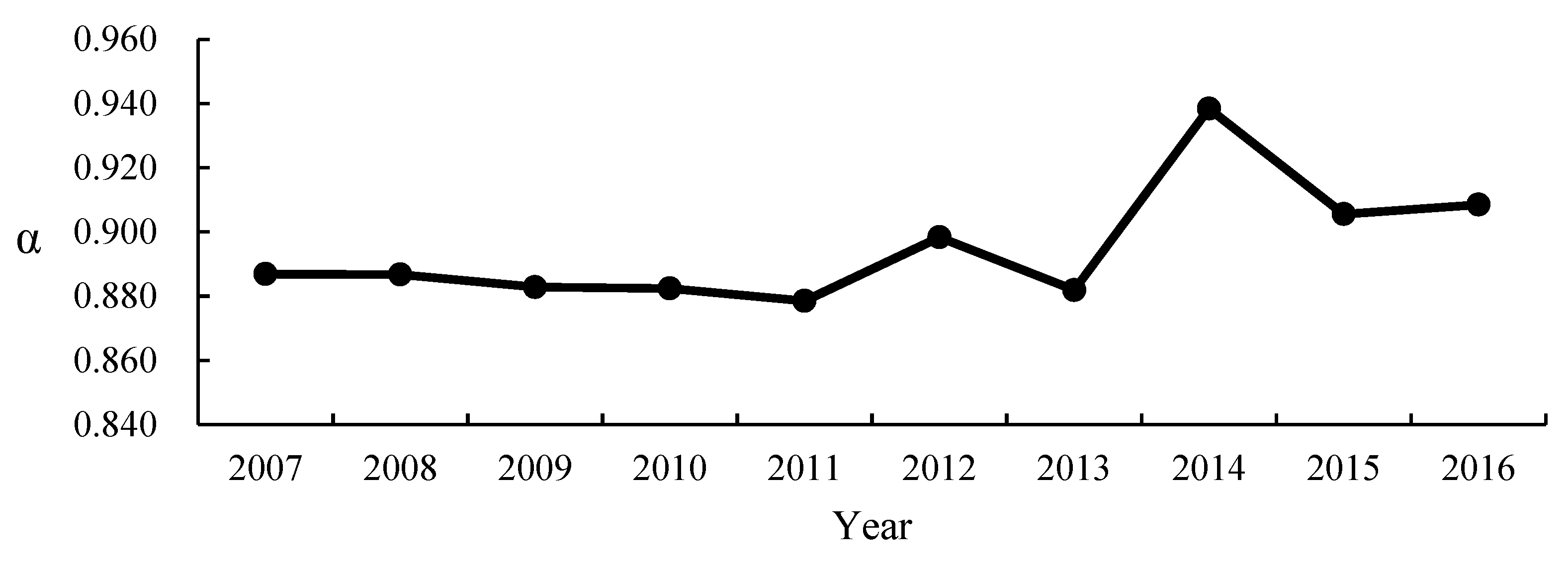With the research deepening, the convergence test, a tool to investigate the evolution of regional disparities, is applied to analyze the regional difference of GHG emissions [38,39,40]. Yang estimates the amount and intensity of agricultural carbon emissions in China from 1993 to 2011, and confirms that there is no α convergence and conditional β convergence in the intensity [41]. Cheng et al. study the convergence trend of agricultural carbon productivity in China from 1997 to 2012, whose results show that there is no α convergence but absolute β convergence [42]. While Wu et al. take the slack based measure under undesirable outputs (SBM-Undesirable) to evaluate China’s agricultural carbon emissions’ performance from 2000 to 2014 and believe that there is no stochastic convergence in carbon emissions or its performance [43]. As seen from the convergence study, scholars concentrate on agricultural GHG emission, paying insufficient attention to absorption, and seldom consider the net effect. Besides, scholars assume that emissions are independent in different regions, so they apply ordinary panel econometric methods when conducting the β convergence test. In fact, agricultural GHG is more likely to correlate spatially because of the similar resource endowments, industrial structure and the emission-mitigation policy imitation in neighboring provinces. If the potential spatial correlation is ignored, it may affect the accuracy of the results [44].

To make up for the existing research, we comprehensively took 21 sources of agricultural GHG emissions into consideration, and linked up the emission and absorption of agricultural ecosystem, to estimate the net GHG emissions of 30 provinces in China from 2007 to 2016. Then, we chose the Moran’s I based on the distance reciprocal square matrix to explore the spatial agglomeration of the emissions. Finally, the convergence theory and spatial econometric methods were used to analyze the emissions’ convergence, aiming to offer a reference for controlling the emissions from both temporal and spatial perspectives. The article is structured as: Section 2 introduces the method and data involved in this study. The third section presents the empirical analysis. The fourth section discusses the results and the last section gives the conclusions.

2. Method and Data

2.1. Calculation of Agricultural Net GHG Emission

Agricultural GHG emission refers to the greenhouse gases released into atmosphere by agricultural production, while agricultural GHG absorption is the greenhouse gases absorbed by crops through photosynthesis, especially carbon dioxide. Both of them act on the net amount, when GHG released minus that of absorbed is positive, agriculture ecosystem is a GHG source, and the corresponding amount is called net emission. On the contrary, when the agriculture ecosystem becomes a GHG sink, the corresponding amount is net absorption.

2.1.1. Agricultural GHG Emission

Four major categories of agricultural GHG emission sources were considered, totaling 21 items. First, carbon emission caused by farmland utilization, involving the input of agricultural materials, the plowing and irrigation activities; second, CH₄ produced during the growth of rice; third, CH₄ and N₂O from intestinal fermentation and fecal management in ruminant breeding; fourth, carbon emissions from agricultural energy. The total GHG emission was the sum of the emissions from 21 sources of four categories mentioned above.

The emissions of each category can be calculated as:

$$E_i={\displaystyle \sum E_j}={\displaystyle \sum (T_j}\cdot {\delta }_j)$$

(1)

where E_i is the total emissions of a certain category; E_j is the emissions of the source j belonging to this category; T_j and δ_j represent the amount and coefficient of the source j, respectively. For the readers interested in the details of the emission coefficient, we list all the coefficients in Appendix A.

To facilitate the analysis, the estimated GHG emissions were boiled down into carbon equivalents, in line with Intergovernmental Panel on Climate Change (IPCC) [45], such that the GHG effect caused by 1 t N₂O and 1 t CH₄ is equivalent to that caused by 298 t CO₂ (81.2727 t C) and 25 t CO₂ (6.8182 t C), respectively [46].

2.1.2. Agricultural GHG Absorption

In terms of the agricultural GHG absorption, we considered the carbon dioxide that crops absorb by photosynthesis in a life cycle, whose calculation equation is:

$$C={\displaystyle \sum _{i=1}^k{C}_i}={\displaystyle \sum _{i=1}^k{c}_i{Y}_i}(1-r_i)/H{I}_i,$$

(2)

where, $C$ is the total amount of carbon dioxide absorbed by crops, C_i is the amount of carbon absorbed by a certain crop, and $c_i$ is the corresponding coefficient of absorption, Y_i, $r_i$, $H{I}_i$ is the economic yield, moisture content factor and economic coefficient of crop i, respectively. The corresponding coefficients can be referred to in

Table A5. Moisture content factor, carbon absorption rate and economic coefficient of main crops.

Crop	Moisture Content Factor	Carbon Absorption Rate	Economic Coefficient
Rice	0.12	0.414	0.45
Wheat	0.12	0.485	0.40
Core	0.13	0.471	0.40
Beans	0.13	0.450	0.34
Rapeseed	0.10	0.450	0.25
Peanut	0.10	0.450	0.43
Sunflower	0.10	0.450	0.30
Cotton	0.08	0.450	0.10
Yams	0.70	0.423	0.70
Sugarcane	0.50	0.450	0.50
Beet	0.75	0.407	0.70
Vegetables	0.90	0.450	0.60
Melons	0.90	0.450	0.70
Tobacco	0.85	0.450	0.56
Other crops	0.12	0.450	0.40

Data source: Wang [22].

of Appendix A.

2.2. Spatial Correlation

To reveal the spatial correlation of agricultural net GHG emissions, Moran’s I autocorrelation analysis was adopted in this paper. We provide the calculation of Moran’s I in Appendix B.

Before calculating Moran’s I, we needed to quantify the spatial relationship of geographic units by spatial weight matrix. When setting the matrix, related research often applies the “0–1” adjacency matrix, which only considers the adjacent relation but ignores the difference caused by geographical distance [47]. Instead, based on the distance attenuation function, we took the reciprocal of the distance square among geographic centers of 30 provinces as the spatial weight, so as to consider the possible interaction among provinces which were geographically close but not adjacent.

2.3. Convergence Test

2.3.1. α Convergence Test

α convergence reflects the deviation of regional agricultural net GHG emissions from the overall average level. In this paper, we explored the convergence or divergence of agricultural net GHG emissions by testing the α coefficient, which denoted the average deviation of each value from the mean. The equation is as:

$$\alpha =\sqrt{\left[{\displaystyle \sum _i(\ln E_{it}}-\overline{\ln E_t}{)}^2\right]/N}$$

(3)

where, ln E_it is the logarithmic value of the agricultural net GHG emissions of the province i in period t, $\overline{\ln E_t}$ is the logarithmic value of the average emissions of all provinces during period t, N is the number of provinces. It was possible to calculate the α value for every year, and if the value gradually decreased with the passage of time, it suggested the agricultural net GHG emissions showed α convergence, otherwise, α convergence did not exist.

2.3.2. Conditional β Convergence Test

β convergence consists of absolute β convergence and conditional β convergence. Absolute β convergence is used to judge the relationship between the growth rate and the initial level of the net emissions, and if they were related negatively, it indicated that there was an absolute β convergence and a catch-up trend existed in backward areas. Different from absolute β convergence, conditional β convergence does not only take the primary level into account, but considers several factors that may also affect the convergence. To explore the influence of different factors, we selected the conditional β convergence test, which can be calculated by Equation (4):

$$\ln \left(\frac{E_{it}}{E_{i,t-1}}\right)=\alpha +\beta \ln (E_{i,t-1}) +\gamma X+{\mu }_i+{\lambda }_t+{\epsilon }_{it}$$

(4)

where, E_it and E_i,t−1 are net agricultural GHG emissions in the t and t − 1 years of the province i, respectively. X represents a set of control variables, and γ is the corresponding parameter; μ_i is the individual-fixed effect and λ_t is the time-fixed effect; ε_it is the error term. If β is negative and statistically significant, it indicates that negative correlation exists between the growth rate and the primary level, which means there is conditional β convergence, if not, conditional β convergence does not exist.

Due to the technology diffusion and the policy imitation of neighboring regions, there may have been spatial correlation of agricultural net GHG emissions. Therefore, when conducting conditional β convergence tests, it was necessary to adopt spatial econometric models, and we mainly considered the spatial lag model (SAR) and spatial error model (SEM), which can be estimated by Equations (5) and (6) respectively.

$$\ln \left(\frac{E_{it}}{E_{i,t-1}}\right)=\alpha +\rho \mathrm{W}\ln \left(\frac{E_{it}}{E_{i,t-1}}\right)+\beta \ln \left(E_{i,t-1}\right)+\gamma X+c_i+{\eta }_t+{\epsilon }_{it}$$

(5)

where, ρ is the spatial autoregressive coefficient, which measures the mutual influence of the growth rates of the net emissions among provinces. The meanings of other variables are the same as in Equation (4).

$$\ln \left(\frac{E_{it}}{E_{i,t-1}}\right)=\alpha +\beta \ln \left(E_{i,t-1}\right)+\gamma X+c_i+{\eta }_t+{\mu }_{it},{\mu }_{it}=\lambda \mathrm{W}{\mu }_{it}+{\epsilon }_{it}$$

(6)

where, λ is the coefficient of spatial error, which is used to measure the spatial correlation degree of error terms. The meanings of other variables are consistent with Equation (4). Elhorst suggested the selection of models could refer to Lagrange multiplier (LM) test: if the LM test statistics (or robust LM test statistics) of spatial lag effect is more significant than that of spatial error effect, SAR should be selected; on the contrary, SEM is more suitable [48]. In addition, the model can be selected according to R², log likelihood, Akaike Information Criterion (AIC), Schwarz Criterion (SC) and other indicators.

In terms of variables, the logarithm of the growth rate of the net emissions was taken as the explained variable, and the logarithm of the net emissions was the core variable. Referring to the relevant studies [33,34,35], we chose six factors that may have affected the convergence of emissions as control variables, as shown in

Table 1. Description of control variables for the conditional β convergence test.

Control Variable	Symbol	Calculation	Unit
Agricultural labor	al	Agricultural practitioners	104 capita
Multiple cropping	mc	Ratio of sown area to cultivated area of crops	-
Agricultural disaster	ad	Ratio of agricultural disaster area to crop sowing area	-
Agricultural economy	ae	Ratio of gross agricultural output value to rural population	104 CNY per capita
Industrial structure	is	Ratio of non-crop production value to gross agricultural output value	-
Fiscal expenditure	fe	Ratio of agricultural fiscal expenditure to total fiscal expenditure	-

Note: To guarantee the gross agricultural output value and the non-crop production value was comparable, it was necessary to convert the corresponding value of each year into the actual value calculated at the comparable price in 2007. To make sure the data was smooth, two variables, agricultural labor and agricultural economy, needed to be logarithmized.

.

2.4. Data Source

Excluding Hong Kong, Macao, Taiwan and Tibet due to missing data, the primary data covers 30 provinces of China from 2007 to 2016, consisting of all kinds of activity data involved in the calculation of agricultural GHG emissions and absorption, and the control variables of β convergence test. The data is introduced in

Table 2. Introduction of data involved in the study.

Calculation	Category	Indicator	Source
Agricultural GHG emissions	Farmland utilization	Application amount of fertilizers, pesticides, plastic mulch, plowing area and irrigation area	China Rural Statistical Yearbook
	Rice planting	Planting area of rice in all provinces	China Rural Statistical Yearbook and National Compilation of Cost and Income Information on Agricultural Products
	Ruminant breeding	Year-end stock of cattle, horses, donkeys, mules, pigs, goats and sheep	China Animal Industry Yearbook and Provincial Statistical Offices
	Agricultural energy consumption	Amount of coal, coke, crude oil, gasoline, kerosene, diesel oil, fuel oil and natural gas used in agricultural production	China Energy Statistics Yearbook and Provincial Statistical Offices
Agricultural GHG absorption	Main crops	Yield of rice, wheat, corn, soybean, rapeseed, peanut, sunflower, cotton, potato, sugar cane, beet, vegetable, melon, tobacco and other crops	China Rural Statistical Yearbook and National Compilation of Cost and Income Information on Agricultural Products
Conditional β convergence test	Control variables	Crop sown area, cultivated land area, agricultural disaster area, gross agricultural output value, total rural population, non-crop production value, fiscal expenditure on agriculture and total fiscal expenditure	China Rural Statistical Yearbook

.

3. Empirical Analysis

3.1. Calculation and Analysis of Agricultural Net GHG Emissions

3.1.1. The Structure of Agricultural Net GHG Emissions

According to the method above, we estimated the net GHG emissions of agriculture in China from 2007 to 2016 and analyzed the structure, as Figure 1 exhibits.

Figure 1 presents the development of agricultural GHG emission and absorption in China. As for emission, the GHG emissions from farmland utilization averaged 52,383.423 × 10⁴ t, accounting for 34.494% of the total GHG emission, which was the largest emissions source. While the source with the smallest emissions was the agricultural energy, with an average of 23,897.309 × 10⁴ t, only accounted for 15.736% of the total. Besides, the mean of the other two sources were 32,850.876 × 10⁴ t and 42,732.930 × 10⁴ t separately, contributed 21.632% and 28.139% of the total amount. Observing the evolution of the structure, the variation trend of GHG emission sources was significantly different. Except the emissions from rice planting, which slightly decreased with an annual decline rate of −0.025%, those from farmland utilization, ruminant breeding and agricultural energy all performed a fluctuating rise, whose annual growth rate were 1.287%, 1.437%, 2.614%, respectively. As for crop GHG absorption, its average amount was 18,616.541 × 10⁴ t, which rose stably during the research period with an annual growth rate of 2.129%. In the agricultural GHG emission structure of China, the amount of absorption was much lower than emissions.

3.1.2. Temporal Evolution of Agricultural Net GHG Emissions

To understand the temporal evolution of the net emissions, the corresponding box-plot was drawn (Figure 2).

The average of provincial net emissions was 4999.916 × 10⁴ t during 10 years. In 2007, the net emission was 4520.424 × 10⁴ t, at the valley in 10 years, and then increased steadily, reaching the 10-year peak of 5842.196 × 10⁴ t in 2014, declined in 2015 and recovered slightly in 2016, showing a fluctuating trend on the whole. Observing the extremum of agricultural net GHG emissions, there was a significant difference among provinces in different years. The minimum did not change significantly and stabilized at about 500.000 × 10⁴ t, while the maximum experienced two light fluctuations, reaching the valley of 10,170.893 × 10⁴ t in 2007 and the peak of 13,104.337 × 10⁴ t in 2014. As can be seen from the interquartile range, the gap of the net emissions among provinces in China was gradually widening.

3.1.3. Spatial Distribution of Agricultural Net GHG Emissions

To show the spatial pattern of agricultural net GHG emissions, we divided the provincial average net emissions into five grades from high to low by natural breakpoint method, and the corresponding spatial distribution map was drawn (Figure 3).

Figure 3 shows the spatial distribution of the net emissions in China. From 2007 to 2016, there were four provinces with the highest emissions, namely Henan, Hunan, Shandong and Heilongjiang, where Henan was the only one whose emissions exceeded 10,000.000 × 10⁴ t. There were seven provinces in the second grade, which were Sichuan, Jiangxi, Hubei, etc. The provinces with medium emission consisted of six provinces, including Guangdong, Yunnan, Jilin, etc. Then the next level included seven provinces, followed by Gansu, Guizhou, Zhejiang and so on. Last, six provinces belonged to lowest level, namely Qinghai, Hainan, Ningxia, etc. The regional pattern of the net emissions presented the “center–periphery” pattern described by New Economic Geography. Meanwhile, the provinces with high emissions were mainly agglomerated in the middle reaches of the Yangtze River, which had always been China’s major agricultural production provinces and were also the central area of the agricultural GHG emissions. In addition, the provinces with low emissions were mainly located in the northwest region, whose agriculture were relatively underdeveloped and the GHG emissions caused by agriculture were naturally less. Apart from the two regions, other regions in China were characterized by staggered distribution of provinces at different GHG emission levels. As can be seen from Figure 3, the emissions showed certain agglomeration in space.

3.2. Spatial Correlation Analysis of Agricultural Net GHG Emissions

3.2.1. Global Correlation Analysis

By using Stata 15.0 software, the global Moran’s I of the net emissions from 2007 to 2016 was calculated, and the results are shown in

Table 3. The Moran’s I of agricultural net GHG emissions from 2007 to 2016 in China.

Year	Moran’s I	Z-Statistics	p-Value
2007	0.111	1.507	0.066
2008	0.118	1.583	0.057
2009	0.128	1.682	0.046
2010	0.122	1.625	0.052
2011	0.128	1.683	0.046
2012	0.171	2.141	0.016
2013	0.127	1.669	0.048
2014	0.147	1.875	0.030
2015	0.123	1.633	0.051
2016	0.133	1.732	0.042

.

The Moran’s I were all over 0.100 and passed the Z-test at a significance level of 10%, which indicated that the agricultural net GHG emissions among provinces were not independent. Due to the similar natural resource, climate conditions and cropping structure, the net emissions became relevant in close provinces. In addition, the global Moran’s I performed unstably, whose value gradually rose in the early years but decreased recently, showing an inverted U-shaped curve overall. Owing to the extensive mode of agricultural production and the single way of emission mitigation, the development of agricultural net GHG emissions behaved similarly among close provinces in the early years. However, with the promotion of environmental protection, various provinces had formulated diversified measures for emission reduction according to their own orientation, resulting in a gradual decrease of net emissions’ correlation.

3.2.2. Local Correlation Analysis

It was hard to describe the specific spatial correlation by global Moran’s I, so we took the 10-year average emissions of 30 provinces as the study objects, and chose the Moran scatter plot to investigate the local spatial correlation, as shown in Figure 4.

The Moran’s I scatter plot included four quadrants, corresponding to “high–high” agglomeration (H–H), “low–high” agglomeration (L–H), “low–low” agglomeration (L–L) and “high–low” agglomeration (H–L) in turn. From Figure 4, the scatters in the first and third quadrants were more than those in the other two quadrants, i.e., the provinces belonging to the “high–high” and the “low–low” agglomeration took the majority. Among them, the provinces whose scatters were located the first quadrant totaled up to eight provinces, including Jilin, Jiangsu, Anhui, etc., showing the trend that high emission areas were surrounded by similar ones. The provinces belonging to the second quadrant included Shanxi, Liaoning, Fujian, etc., owning the character that low emission areas were surrounded by high emission areas. The provinces in the third quadrant comprised of Beijing, Tianjin, Shanghai and so on, performing that the low emission areas were surrounded by the similar ones. The provinces of the fourth quadrant included Hebei, Inner Mongolia, Sichuan and so on, which were characterized by high emission areas surrounded by those who performed oppositely. To conclude, the provinces of “high–high” agglomeration were mainly situated in the middle reaches of the Yangtze River, while those of “low–low” agglomeration mainly located in the northern coastal, eastern coastal and northwest regions. In addition, provinces around the country showed obvious polarization of high-value and low-value agglomeration.

Aiming to distinguish the agglomeration under the significance level of 5%, we selected the base year (2007), the last year (2016), the year with the strongest (2012) and the weakest spatial correlation (2007), and then drew the corresponding Lisa agglomeration maps, as shown in Figure 5.

As seen from Figure 5, under the 5% significance level, the provinces showing significant agglomeration had decreased sharply. There were mainly two types of agglomeration left, as the net emissions in middle reaches of the Yangtze River mainly exhibited “high–high” agglomeration, and those in the northern coastal region appeared to show “low–low” agglomeration, indicating that an obvious polarization existed. With the passage of time, the spatial correlation pattern had changed greatly. Specifically, in 2007, the spatial correlation was the weakest. The “high–high” agglomeration areas included Jiangxi, Hubei and Hunan provinces, while Beijing and Tianjin showed “low–low” agglomeration. By 2012, Beijing and Tianjin continued to be the “low–low” agglomeration centers, and Henan became a new center of “high–high” agglomeration. Besides, Hebei, as a transitional area of two agglomerations, was significantly characterized by “high–low” agglomeration. By 2016, the pattern of “low–low” and “high–high” agglomeration had not changed, but the “high–low” agglomeration in Hebei was no longer significant.

3.3. Convergence Test

The analysis above suggested that there were apparent gaps of the net emissions in different provinces, but they showed local spatial correlation in space. Then, with the passage of time, would the gaps narrow naturally? We applied α convergence test and conditional β convergence test to explore the gaps of the net emissions among provinces.

3.3.1. α Convergence Test

The α coefficient of China’s agricultural net GHG emissions was calculated year by year, and we drew a corresponding line chart, as shown in Figure 6.

Observing Figure 6, the α coefficient of the net emissions showed an overall upward tendency during the research period, indicating that there was no α convergence among 30 provinces. As the emissions developed diversely in different provinces, the gaps among provinces would continue to widen. Besides, the gaps diverged in different periods: the α coefficient decreased slowly from 0.887 to 0.879 in the first five years, showing weak convergence, while it presented fluctuating growth during the recent period, with a peak of 0.938 in 2014, which suggested that the evolution of agricultural net GHG emissions’ gaps was unstable.

3.3.2. Conditional β Convergence Test

There was no α convergence for the national net emissions, which implied that the emission level of all provinces would not converge to a same stable standard. Then, we eased the convergence conditions and tried a conditional β convergence test, aiming to examine whether the “chase effect” of the emissions existed among provinces. The Moran’s I estimation confirmed that emissions showed a positive spatial autocorrelation in provinces, so the conditional β convergence analysis should be conducted by the spatial econometric methods, instead of the ordinary panel econometric model. In this paper, Stata 15.0 software was used for spatial econometric analysis, and we conducted spatial relevant tests for selecting spatial econometric models, which are shown in

Table 4. The results of spatial panel econometric model test.

Test	χ2	p-Value
LM Error (Burridge)	1.730	0.188
LM Error (Robust)	1.539	0.215
LM Lag (Anselin)	19.764	0.000
LM Lag (Robust)	19.572	0.000

.

As the Table 4 presents, the statistics of spatial lag effect were both significant at the 1% statistic level, while those of spatial error effect were not, so SAR was more suitable for convergence analysis. The data was a short panel of data, so there was no need for a panel unit root test or co-integration test. To ensure the robustness of the empirical results, the estimation of SEM and the ordinary panel econometric model was taken as the comparison. The Hausman statistics of the three models were significant at the 1% statistic level, all accepting the hypothesis of fixed effects. The regression results were exhibited in

Table 5. The results of conditional β convergence tested by three econometric methods.

Variables	SAR	SEM	Ordinary Panel Model
ln (emissions)	0.521 ***	0.737 ***	0.494 ***
	(3.57)	(3.06)	(6.93)
mc	−0.023	−0.023	−0.020
	(−1.11)	(−1.07)	(−0.90)
ln (al)	−0.231 ***	−0.312 **	−0.194 **
	(−2.89)	(−2.38)	(−2.58)
ad	−0.027	−0.048	−0.041
	(−0.77)	(−1.02)	(−1.23)
ln (ae)	−0.114 ***	−0.171 **	−0.123 ***
	(−2.80)	(−2.27)	(−4.88)
is	−0.042	−0.142	0.230
	(−0.21)	(−0.91)	(0.57)
fe	0.544	0.785	0.532
	(1.09)	(0.99)	(1.40)
ρ/λ	0.547	0.638	-
	(5.86)	(6.21)	-
Hausman	102.960	47.050	157.520
R2	0.518	0.373	0.392
Log-likelihood	379.696	371.070	-

Note: Z-statistics are presented in the brackets; *** and ** mean variables were significant at 1% and 5% statistical levels, respectively.

, where the log-likelihood ratio of SAR was 379.696, higher than that of SEM, and the R² was 0.518, better than the other two models, which also supported the rationality of SAR. Most of the variable coefficients of the three models presented the same sign and little numerical difference, indicating that the estimation results were robust.

Observing the estimation results of the SAR, we found the coefficient of emission’s logarithm was positive at a 1% significance level, which proved the national agricultural net GHG emissions did not show conditional β convergence, that is, there was no “chase effect” among provinces. Due to the differences of resource endowments, economic development and industrial structure, not only did backward regions have higher net emissions than advanced regions in the primary stage, but the gap continued to widen over time. In addition, the spatial autoregressive coefficient ρ was 0.547 and passed the Z-test at the 1% significance level, implying the growth rates of the net emissions inclined to show spatial spillover effect significantly in close provinces.

As for the control variables, the coefficients of agricultural labor and agricultural economy were both negative and significant at the statistical level of 1%, indicating that the expansion of labor and the improvement of economy were conducive to lowering the growth rate of the net emissions. As the agricultural practitioners decrease, machines of irrigating and plowing would make up for the reduced labor in the agricultural production, suggesting that the GHG emissions caused by agricultural energy, such as diesel oil and agricultural gasoline, would increase. From the reality in China, with the acceleration of urbanization and more agricultural labor force transferring to the industry, the growth rate of agricultural net GHG emissions would be significantly increased. The development of agricultural economy also had a negative effect on the growth rate of net emissions. With the development of agricultural economy, green and clean mode of intensified production had been gradually replacing the extensive operation mode with excessive energy consumption and large emissions, which contributed to the emission mitigation.

4. Discussion

4.1. Implication

Agricultural GHG emissions plays an important role in global warming. As can be seen from the analysis, the situation of agricultural GHG in China is not optimistic, which reveals the urgency to accelerate the pace of emission mitigation.

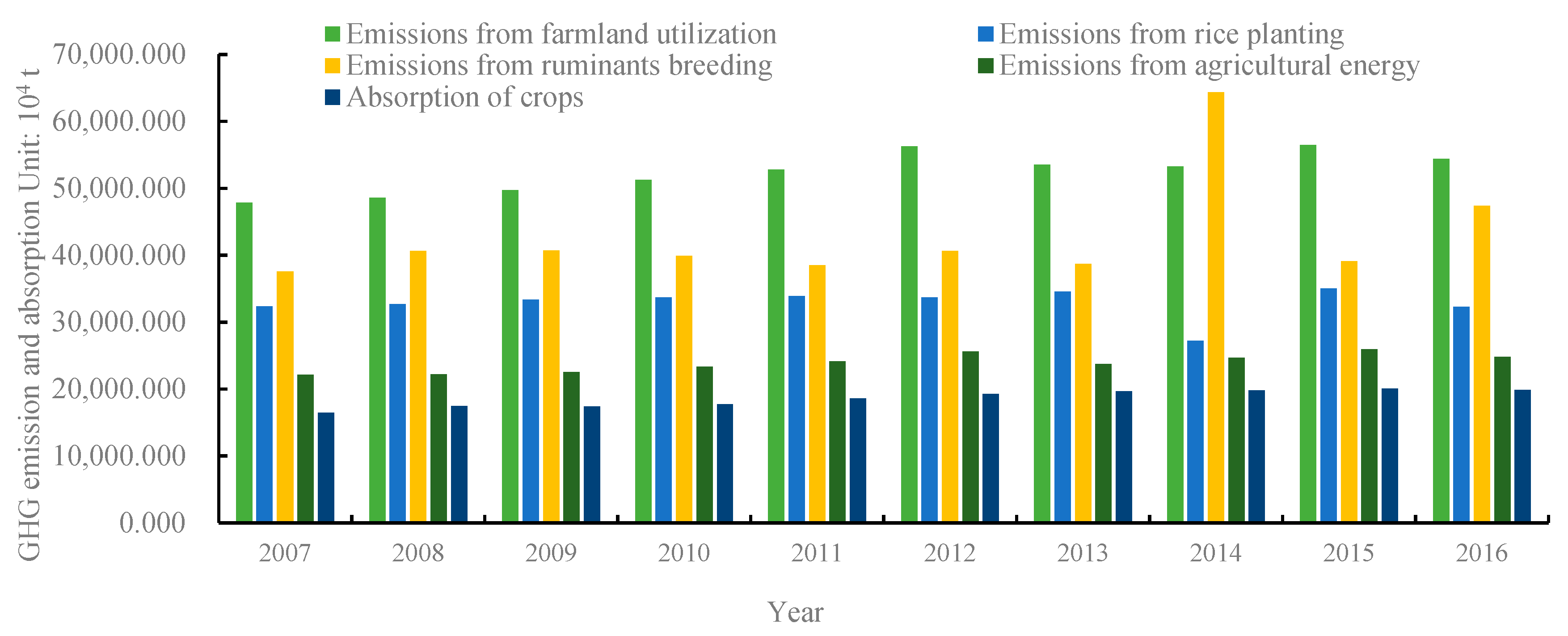
(1) Although agricultural net GHG emissions in China had experienced some ups and downs in the sample years, it showed an overall upward trend. Moreover, based on the evolution, we could predict the net emissions may continue to grow in the next few years, manifesting the necessity to take measures for emissions mitigation. From the structure, GHG emissions from farmland utilization, ruminant breeding and agricultural energy all showed growing trends, especially those from farmland utilization, accounting for 34.494% of the total amount, should be paid more attention.

(2) Due to the obvious provincial difference, when formulating regional agricultural GHG emission mitigation policies, it is essential to establish differentiated emission reduction targets based on local conditions. The key is to apply the low-carbon development mode of farming: adjust agricultural production structure and plant low-emission and high-sink crops that adapt to local resources, increase investment in technology to enhance the efficiency of agricultural machinery and the utilization rate of energy, encourage agricultural practitioners to learn conservation-oriented fertilization techniques, use pesticides rationally and recycle the waste plastic mulch.

(3) Based on the results of two convergence tests, there is no convergence nationwide, so it is hard for the net emissions to reduce naturally. On the contrary, taking effective reduction measures is a possible way to bridge the provincial gaps. Besides, the net emissions showed spatial correlation, which interact and influence each other among provinces, suggesting that there is a possibility of regional cooperation. It is necessary for all regions to strengthen cooperation and share low-carbon technology, so as to cut down the net emissions coordinately through provincial correlation.

(4) A series of studies showed that some technologies may act in carbon sequestration and negative emission of carbon may be achieved [49]. Technologies and techniques as biochar [49], agroforestry systems [50] and conservational agriculture measurements [51,52] may act as additional benefit methods for reduce carbon emission in agriculture. At present, low-carbon technology is relatively insufficient for agriculture in China, and most of them are staying in the experimental stage. In the future, China should attach importance to the development of the technologies and techniques and apply them to practice as soon as possible.

4.2. Comparison

Comparing with the existing estimation of China, we find that difference in categories and sources of agricultural GHG leads to the diversity of the results. Taking Chen’s estimation for example, he deems that China’s agriculture served as a net GHG sink from 1991 to 2011 [30], while we believe that it was a GHG source from 2007 to 2016. Observing the calculation procedure, Chen calculates the GHG absorption from 15 kinds of crops, whose categories and corresponding coefficients are the same as our study, but there is a difference when calculating the emissions: Chen’s research is on the basis of six sources of GHG emission source, inclusive of fertilizer, pesticide, plastic mulch, sheep, cow and pig, less than our study that considers 21 sources of GHG emissions. Therefore, there is little difference in the estimation of absorption between the two studies, but the emissions we estimated are much more than Chen’s, consequently causing a significant difference in the net amount.

As for convergence, previous research focus on GHG emissions and relative indicators, and some scholars have agreed that the agricultural GHG emissions of China does not achieve convergence nationwide, neither does the intensity or performance [41,43], while the national agricultural carbon productivity has absolute β convergence [42]. Instead, we took the net emissions as the target, and found that neither of α convergence or conditional β convergence existed in the whole country, which is a complement to the existing research.

4.3. Improving Direction

It should be noted that there are some limitations of this study. First, it lacks the consideration for GHG effect of soil. The emission and sequestration of soil is closely related to the farming system, where the soil carbon loss caused by no-tillage, less tillage or complete cultivation often has a world of difference [34]. Some scholars adopt the test data of a certain region as GHG emission coefficient of soil, and applied it to the whole country [4,53]. However, China has a vast territory, and its geographical conditions and production patterns are quite different. Therefore, the application of such a simple way is unscientific. Based on the above reasons, GHG emission and sequestration of soil have not been considered in our measurement system of the agricultural GHG net emission.

Second, the impact of different farming methods was not considered. The agricultural practices, such as cover crops and straw returning, may also influence the carbon sequestration in the soil, resulting in a completely different net effect of GHG. As the major mode in China is smallholder production, it was hard to consider the influence of cultivation modes in different regions. For this reason, this paper did not consider different agricultural practices, which may have led to deviation in the result.

To refine the measurement system and ensure the accuracy of results, we will focus on taking the GHG effect of soil into research in the future. In addition, assessing the influence of different agricultural practices also becomes the next direction.

5. Conclusions

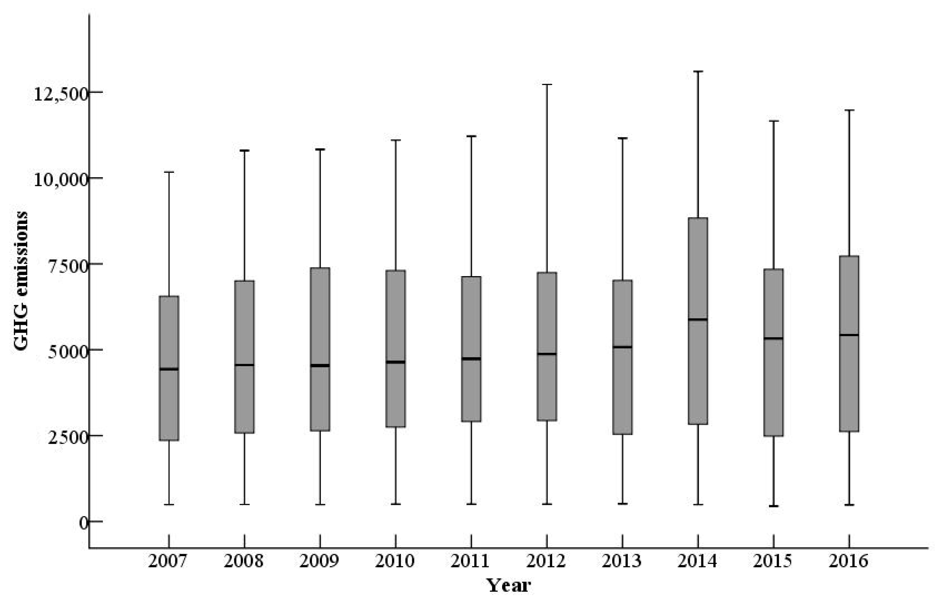
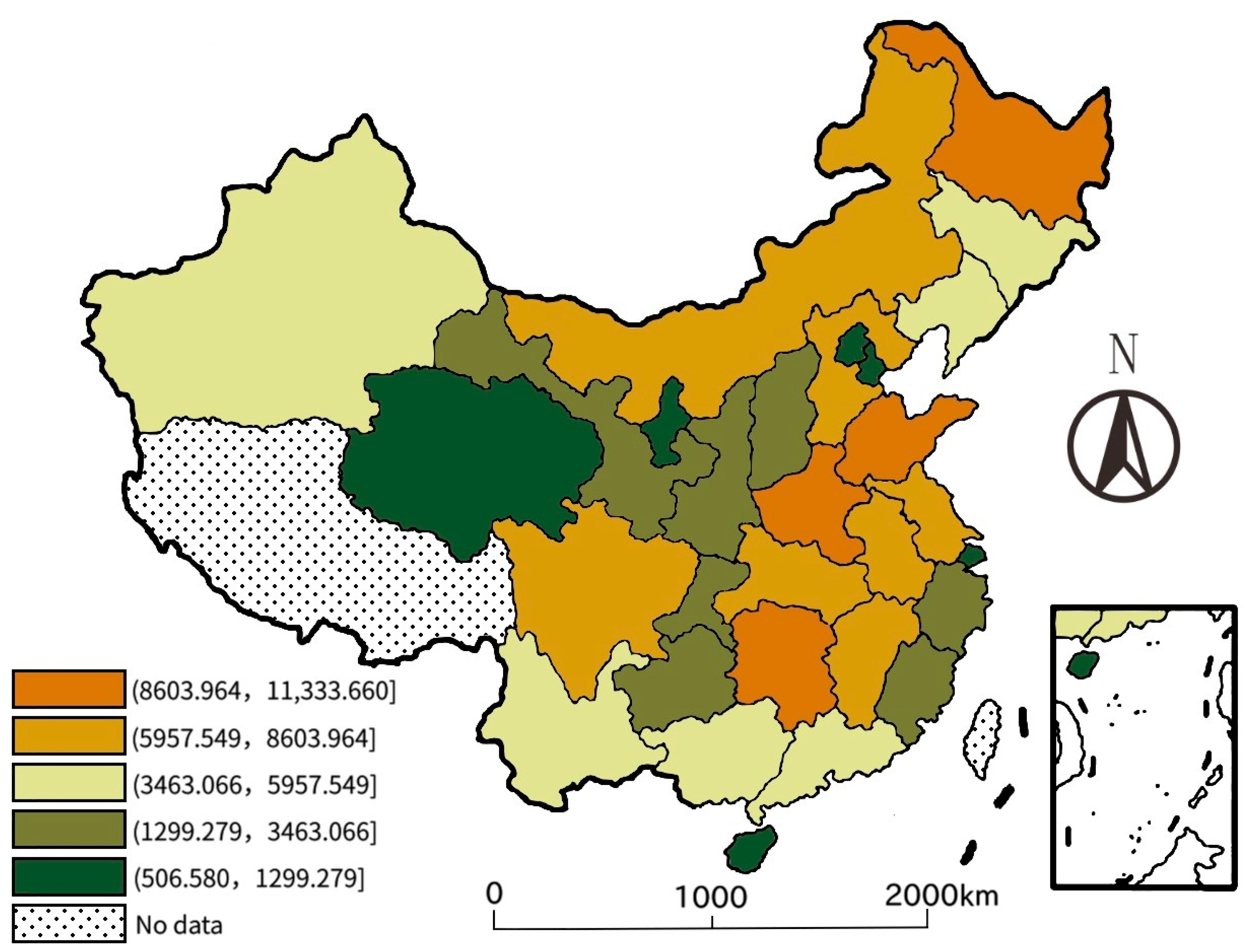
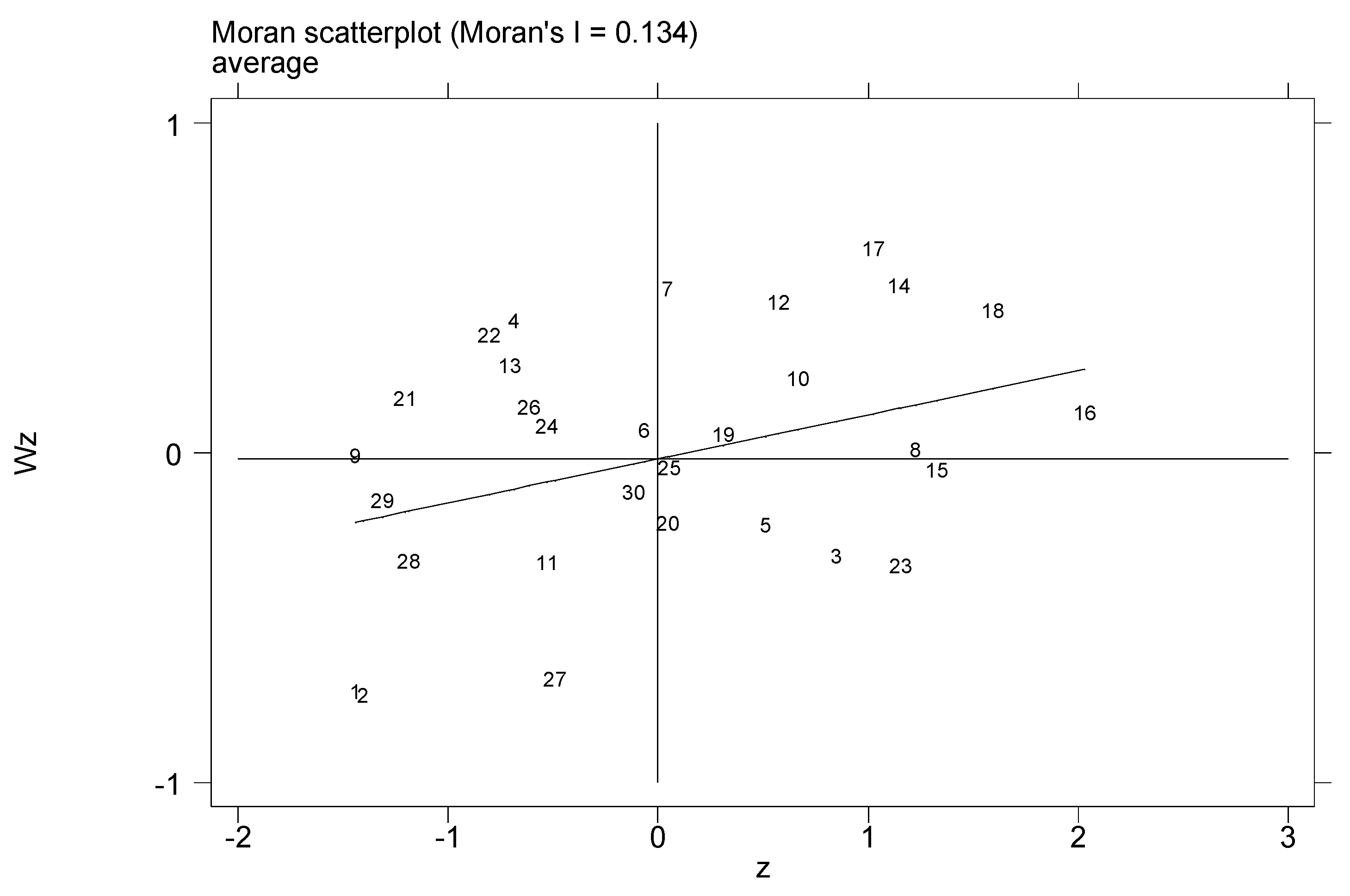
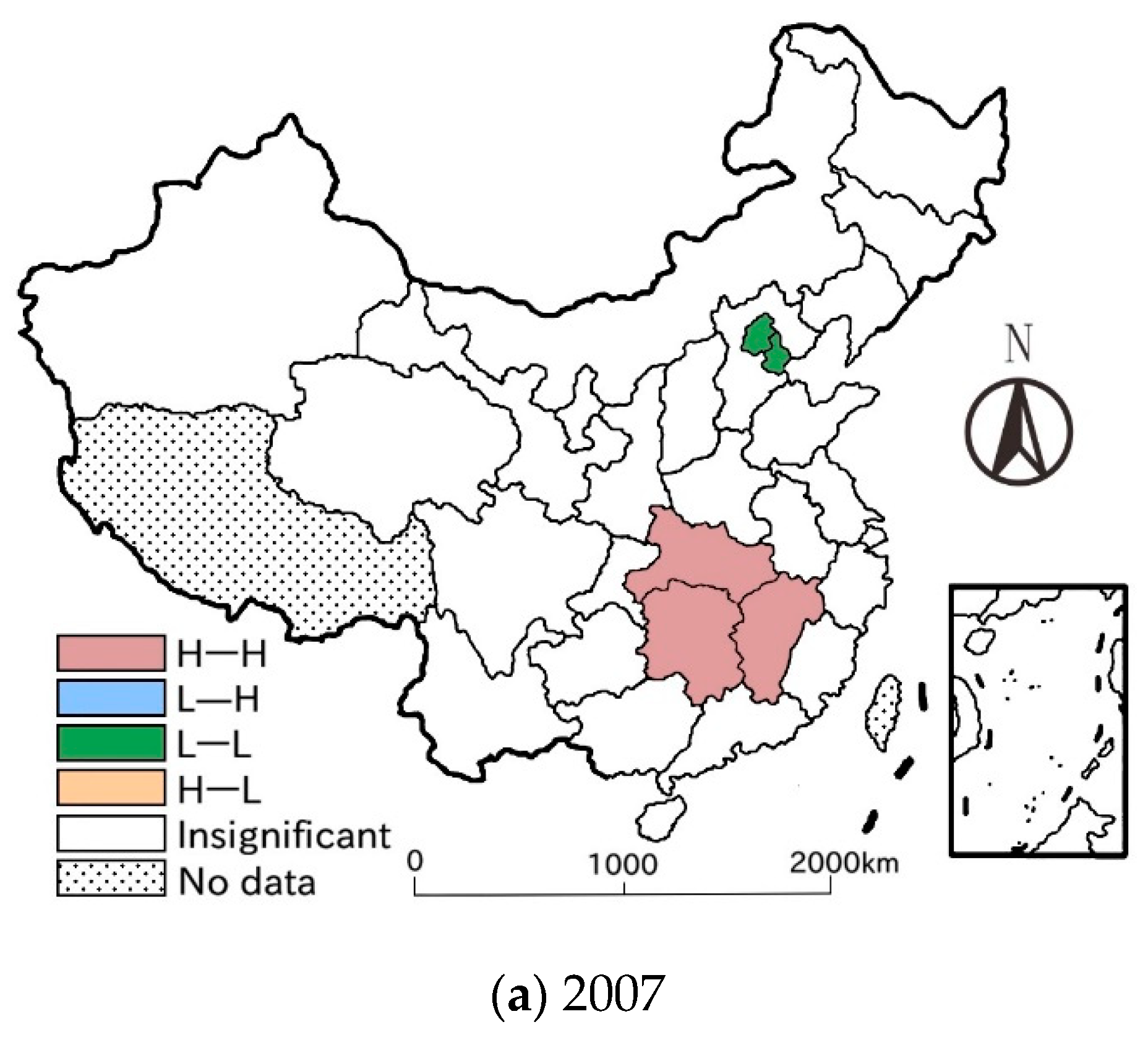
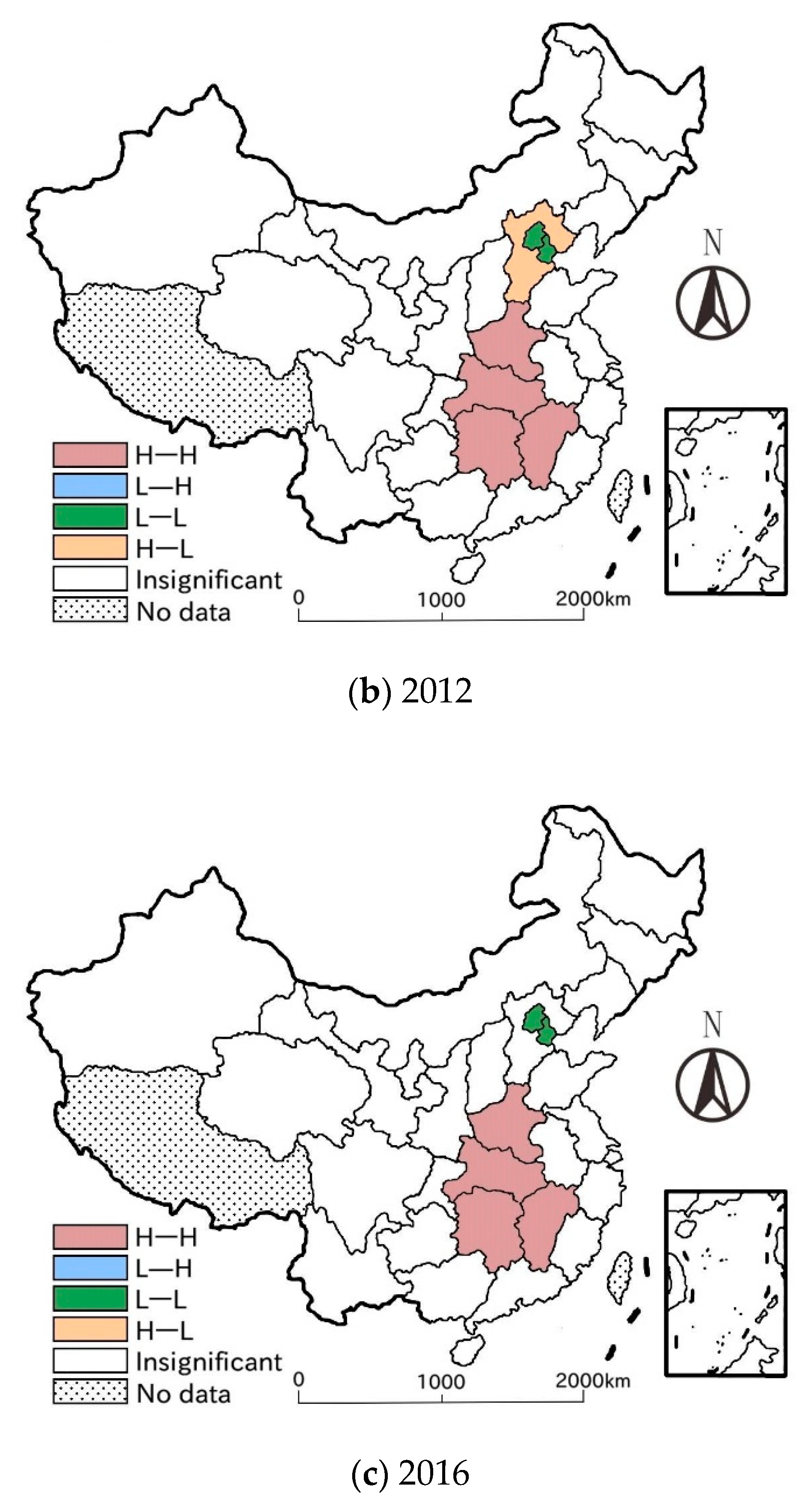
Based on the Moran’s I, convergence tests and spatial econometric models, the study analyzed the spatial correlation and convergence of agricultural net GHG emissions in China. From 2007 to 2016, the average of the net emissions of all provinces was 4999.916 × 10⁴ t, showing a fluctuating growth trend as a whole, and the gaps among provinces had been gradually widening. Most of the provinces with large emissions belonged to the middle reaches of the Yangtze River, while the provinces with low emissions were mainly located in the northwest of China. As for the spatial correlation, the global Moran’s I of agricultural net GHG emissions was all over 0.100, implying the net emissions were spatially correlated, whose correlation level showed an inverted U-shaped curve as a whole. There was an obvious polarization of the net emissions, mainly exhibiting “high–high” and “low–low” agglomeration, whose agglomerating centers were situated in the middle reaches of the Yangtze River and the northern coastal region respectively. With the passage of time, the spatial correlation pattern had changed greatly. In terms of convergence, agricultural net GHG emissions did not show α convergence or conditional β convergence in the whole country. With time going by, the gaps among different provinces broadened, and there was no “chase effect” in the emissions’ growth rate among provinces. In addition, the growth rate had a significant positive spatial spillover effect in close provinces, and the agricultural force and economic development had negative impact on the growth rate of the net emissions.

References

1. Johnson, M.F.; Franzluebbers, A.J.; Weyers, S.L.; Reicosky, D.C. Agricultural opportunities to mitigate greenhouse gas emissions. Environ. Pollut. 2007, 150, 107–124. [Google Scholar] [CrossRef] [PubMed]
2. Li, B.; Zhang, J.B.; Li, H.P. Research on spatial-temporal characteristics and affecting factors decomposition of agricultural carbon emission in China. China Popul. Resour. Environ. 2011, 21, 80–86. [Google Scholar] [CrossRef]
3. Tubiello, F.N.; Salvatore, M.; Golec, R.D.C.; Ferrara, A.; Rossi, S.; Biancalani, R.; Federici, S.; Jacobs, H.; Flammini, A. Agriculture, forestry and other land use emissions by sources and removals by sinks: 1990–2011 analysis. FAO Stat. Div. 2014, 4, 375–376. [Google Scholar]
4. Tian, Y.; Zhang, J.B. Study on the differentiation of net carbon effect in agricultural production in China. J. Nat. Resour. 2013, 28, 1298–1309. [Google Scholar] [CrossRef]
5. Tongwane, M.; Mdlambuzi, T.; Moeletsi, M.; Tsubo, M.; Mliswa, V.; Grootboom, L. Greenhouse gas emissions from different crop production and management practices in South Africa. Environ. Dev. 2016, 19, 25–35. [Google Scholar] [CrossRef]
6. Goglio, P.; Smith, W.N.; Grant, B.B.; Desjardins, R.L.; Gao, X.; Hanis, K.; Tenuta, M.; Campbell, C.A.; McConkey, B.G.; Nemecek, T.; et al. A comparison of methods to quantify greenhouse gas emissions of cropping systems in LCA. J. Clean. Prod. 2017, 172, 4010–4017. [Google Scholar] [CrossRef]
7. Zhang, X. Multiple cropping system expansion: Increasing agricultural greenhouse gas emissions in the north China plain and neighboring regions. Sustainability 2019, 11, 3941. [Google Scholar] [CrossRef]
8. Lu, X.H.; Kuang, B.; Li, J.; Han, J.; Zhang, Z. Dynamic evolution of regional discrepancies in carbon emissions from agricultural land utilization: Evidence from Chinese provincial data. Sustainability 2018, 10, 552. [Google Scholar] [CrossRef]
9. Lin, H.W.; Jin, Y.F.; Giglio, L.; Foley, J.A.; Randerson, J.T. Evaluating greenhouse gas emissions inventories for agricultural burning using satellite observations of active fires. Ecol. Appl. 2012, 22, 1345–1364. [Google Scholar] [CrossRef]
10. Wang, W.W.; Zhang, J.B.; Wang, P.C. Carbon emission measurement using different utilization methods of waste products: Taking cotton straw resources of south Xinjiang in China as an example. Nat. Environ. Pollut. Technol. 2018, 17, 383–390. [Google Scholar]
11. Kipling, R.P.; Taft, H.E.; Chadwick, D.R.; Styles, D.; Moorby, J. Challenges to implementing greenhouse gas mitigation measures in livestock agriculture: A conceptual framework for policymakers. Environ. Sci. Policy 2019, 92, 107–115. [Google Scholar] [CrossRef]
12. Garnier, J.; Noë, L.J.; Marescaux, A.; Cobena, A.S.; Lassaletta, L.; Silvestre, M.; Thieu, V.; Billen, G. Long-term changes in greenhouse gas emissions from French agriculture and livestock (1852–2014): From traditional agriculture to conventional intensive systems. Sci. Total Environ. 2019, 660, 1486–1501. [Google Scholar] [CrossRef] [PubMed]
13. Bellarby, J.; Tirado, R.; Leip, A.; Weiss, F.; Lesschen, J.P.; Smith, P. Livestock greenhouse gas emissions and mitigation potential in Europe. Glob. Chang. Biol. 2013, 19, 3–18. [Google Scholar] [CrossRef] [PubMed]
14. Smith, W.N.; Grant, B.B.; Desjardins, R.L.; Worth, D.; Huffman, E.C. A tool to link agricultural activity data with the DNDC model to estimate GHG emission factors in Canada. Agric. Ecosyst. Environ. 2010, 136, 301–309. [Google Scholar] [CrossRef]
15. Thamo, T.; Kingwell, R.S.; Pannell, D.J. Measurement of greenhouse gas emissions from agriculture: Economic implications for policy and agricultural producers. Aust. J. Agr. Resour. Ec. 2013, 57, 234–252. [Google Scholar] [CrossRef]
16. Huang, K.-T.; Wang, J.C. Greenhouse gas emissions of tourism-based leisure farms in Taiwan. Sustainability 2015, 7, 11032–11049. [Google Scholar] [CrossRef]
17. Liski, J.; Perruchoud, D.; Karjalainen, T. Increasing carbon stocks in the forest soils of Western Europe. Ecol. Manag. 2002, 169, 159–175. [Google Scholar] [CrossRef]
18. Baritz, R.; Seufert, G.; Montanarella, L.; Ranst, E.V. Carbon concentrations and stocks in forest soils of Europe. Ecol. Manag. 2010, 260, 262–277. [Google Scholar] [CrossRef]
19. Pan, Y.; Birdsey, R.A.; Fang, J.; Houghton, R.; Kauppi, P.E.; Kurz, W.A.; Philips, O.L.; Shvidenko, A.; Lewis, S.L.; Canadell, J.G.; et al. A large and persistent carbon sink in the world’s forests. Science 2011, 333, 988–993. [Google Scholar] [CrossRef]
20. Erb, K.H.; Kastner, T.; Luyssaert, S.; Houghton, R.A.; Kuemmerle, T.; Olofsson, P.; Haberl, H. Bias in the attribution of forest carbon sinks. Nat. Clim. Chang. 2013, 3, 854–856. [Google Scholar] [CrossRef] [Green Version]
21. Luyssaert, S.; Schulze, E.D.; Börner, A.; Knohl, A.; Hessenmöller, D.; Law, B.E.; Ciais, P.; Grace, J. Old-growth forests as global carbon sinks. Nature 2008, 455, 213–215. [Google Scholar] [CrossRef] [PubMed]
22. Wang, X.L. Carbon Dioxide, Climate Change, and Agriculture; China Meteorological Press: Beijing, China, 1996. [Google Scholar]
23. Han, Z.Y.; Meng, Y.L.; Xu, J.; Wu, Y.; Zhou, Z.G. Temporal and spatial difference in carbon footprint of regional farmland ecosystem-taking Jiangsu Province as a case. J. Agro Environ. Sci. 2012, 5, 1034–1041. [Google Scholar]
24. West, T.O.; Marland, G. A Synthesis of carbon sequestration, carbon emissions, and net carbon flux in agriculture: Comparing tillage practices in the United States. Agric. Ecosyst. Environ. 2002, 91, 217–232. [Google Scholar] [CrossRef]
25. Vleeshouwers, L.M.; Verhagen, A. Carbon emission and sequestration by agricultural land use: A model study for Europe. Glob. Change Biol. 2010, 8, 519–530. [Google Scholar] [CrossRef]
26. Wear, D.N.; Coulston, J.W. From sink to source: Regional variation in U.S. forest carbon futures. Sci. Rep. 2015, 5, 16518. [Google Scholar] [CrossRef] [PubMed]
27. Popp, M.; Nalley, L.; Fortin, C.; Smith, A.; Brye, K. Estimating net carbon emissions and agricultural response to potential carbon offset policies. Agron. J. 2011, 4, 1131–1143. [Google Scholar] [CrossRef]
28. Xiong, C.H.; Yang, D.G.; Huo, J.W.; Wang, G.L. Agricultural net GHG Effect and agricultural carbon sink compensation mechanism in Hotan prefecture, China. Pol. J. Environ. Stud. 2017, 1, 365–373. [Google Scholar] [CrossRef]
29. Duan, H.P.; Zhang, Y.; Zhao, J.B.; Bian, X.M. Carbon footprint analysis of farmland ecosystem in China. J. Soil Water Conserv. 2011, 25, 203–208. [Google Scholar] [CrossRef]
30. Chen, L.Y.; Xue, L.; Xue, Y. Spatial agglomeration and variation of China’s agricultural net carbon sink. J. Ecol. Environ. 2015, 11, 1777–1784. [Google Scholar]
31. Neumayer, E. Can natural factors explain any cross-country differences in carbon dioxide emissions? Energy Policy 2002, 30, 7–12. [Google Scholar] [CrossRef] [Green Version]
32. Lantz, V.; Feng, Q. Assessing income, population, and technology impacts on CO2 emissions in Canada: Where’s the EKC? Ecol. Econ. 2006, 57, 229–238. [Google Scholar] [CrossRef]
33. Uchiyama, K. Environmental Kuznets Curve Hypothesis and Carbon Dioxide Emissions; Springer: Tokyo, Japan, 2016. [Google Scholar]
34. Lal, R. Carbon emission from farm operations. Environ. Int. 2004, 30, 981–990. [Google Scholar] [CrossRef] [PubMed]
35. Zhang, J.B.; Cheng, L.L.; He, K. The difference of China’s agricultural low-carbon economic efficiency in spatial and temporal and its influencing factors: A perspective of carbon input. J. Environ. Econ. 2017, 2, 36–51. [Google Scholar] [CrossRef]
36. Cole, C.V.; Duxbury, J.; Freney, J.; Heinemeyer, O.; Minami, K.; Mosier, A.; Paustian, K.; Rosenberg, N.; Sampson, N.; Sauerbeck, D.; et al. Global estimates of potential mitigation of greenhouse gas emissions by agriculture. Nutr. Cycl. Agroecosyst. 1997, 49, 221–228. [Google Scholar] [CrossRef]
37. Dace, E.; Muizniece, I.; Blumberga, A.; Kaczala, F. Searching for solutions to mitigate greenhouse gas emisisons by agricultural policy decisions—Application of system dynamics modeling for the case of Latvia. Sci. Total Environ. 2015, 527, 80–90. [Google Scholar] [CrossRef]
38. Strazicich, M.C.; List, J.A. Are CO2 emission levels converging among industrial countries? Environ. Resour. Econ. 2003, 24, 263–271. [Google Scholar] [CrossRef]
39. Westerlund, J.; Basher, S.A. Testing for convergence in carbon dioxide emissions using a century of panel data. Environ. Resour. Econ. 2008, 40, 109–120. [Google Scholar] [CrossRef]
40. Lee, C.C.; Chang, C.P. New evidence on the convergence of per capita carbon dioxide emissions from panel seemingly unrelated regressions augmented Dickey-Fuller tests. Energy 2008, 33, 1468–1475. [Google Scholar] [CrossRef]
41. Yang, X.Y. Regional differences and convergence of agricultural carbon emissions in China. Hubei Agric. Sci. 2016, 55, 1066–1072. [Google Scholar] [CrossRef]
42. Cheng, L.L.; Zhang, J.B.; Zeng, Y.M.; Wu, X.R. Analysis on the dynamic evolution and spatial club convergence of national agricultural carbon productivity. J. Chin. Agric. Univ. 2016, 21, 121–132. [Google Scholar] [CrossRef]
43. Wu, H.Y.; He, Y.Q.; Chen, R. Agricultural carbon emissions performance and its stochastic convergence in China-Based on SBM-Undesirable model and panel unit root test. Chin. J. Ecoagri. 2017, 25, 1381–1391. [Google Scholar] [CrossRef]
44. Anselin, L. Spatial Econometrics: Methods and Models; Kluwer Academic Publishers: Dordrecht, The Netherlands, 1988. [Google Scholar]
45. IPCC. Climate Change 2007: The Physical Science Basis: Working Group I Contribution to the Fourth Assessment Report of the Intergovernmental Panel on Climate Change; Cambridge University Press: New York, NY, USA, 2007. [Google Scholar]
46. Guan, X.L.; Zhang, J.B.; Wu, X.R.; Cheng, L.L. The shadow prices of carbon emissions in China’s planting industry. Sustainability 2018, 10, 753. [Google Scholar] [CrossRef]
47. Wu, X.R.; Zhang, J.B.; Cheng, L.L.; Tian, Y. Potential of agricultural carbon reduction under climate change and its spatial correlation characteristics in China: Based on the spatial Durbin model. China Popul. Resour. Environ. 2015, 25, 53–61. [Google Scholar]
48. Elhorst, J.P. Spatial Econometrics: From Cross-Sectional Data to Spatial Panels; Springer: Berlin, Germany, 2014. [Google Scholar]
49. Smith, P. Soil carbon questionar and biochar as negative emission technologies. Glob. Chang. Biol. 2016, 22, 1315–1324. [Google Scholar] [CrossRef]
50. Albrecht, A.; Kandji, S.T. Carbon sequestration in tropical agroforestry systems. Agric. Ecosyst. Environ. 2003, 99, 15–27. [Google Scholar] [CrossRef]
51. Powlson, D.S.; Stirling, C.M.; Thierfelder, C.; White, R.P.; Jat, M.L. Does conservation agriculture deliver climate change mitigation through soil carbon sequestration in tropical agro-ecosystems? Agric. Ecosyst. Environ. 2016, 220, 164–174. [Google Scholar] [CrossRef]
52. Corbeels, M.; Cardinael, R.; Naudin, K.; Guibert, H.; Torquebiau, E. The 4 per 1000 goal and soil carbon storage under agroforestry and conservation agriculture systems in sub-Saharan Africa. Soil Till. Res. 2019, 188, 16–26. [Google Scholar] [CrossRef] [Green Version]
53. Tan, Q. Greenhouse gas emission in China’s agriculture: Situation and challenge. China Popul. Resour. Environ. 2011, 21, 69–75. [Google Scholar] [CrossRef]
54. Min, J.S.; Hu, H. Calculation of greenhouse gases emission from agricultural production in China. China Popul. Resour. Environ. 2012, 22, 21–27. [Google Scholar]
Figure 1. The histogram of agricultural net greenhouse gas (GHG) emissions’ structure of China from 2007 to 2016.
Sustainability 11 04817 g001
Figure 2. The box-plot of agricultural net GHG emissions of China from 2007 to 2016 (Unit: 104 t).
Sustainability 11 04817 g002
Figure 3. The spatial distribution of agricultural net GHG emissions in China (Unit: 104 t).
Sustainability 11 04817 g003
Figure 4. The local Moran scatter diagram of average agricultural net GHG emissions of 30 provinces. Note: 1 is Beijing, 2 is Tianjin, 3 is Hebei, 4 is Shanxi, 5 is Inner Mongolia, 6 is Liaoning, 7 is Jilin, 8 is Heilongjiang, 9 is Shanghai, 10 is Jiangsu, 11 is Zhejiang, 12 is Anhui, 13 is Fujian, 14 is Jiangxi, 15 is Shandong, 16 is Henan, 17 is Hubei, 18 is Hunan, 19 is Guangdong, 20 is Guangxi, 21 is Hainan, 22 is Chongqing, 23 is Sichuan, 24 is Guizhou, 25 is Yunnan, 26 is Shaanxi, 27 is Gansu, 28 is Qinghai, 29 is Ningxia and 30 is Xinjiang.
Sustainability 11 04817 g004
Figure 5. Lisa agglomeration map of agricultural net GHG emissions in China in 2007, 2012 and 2016.
Sustainability 11 04817 g005aSustainability 11 04817 g005b
Figure 6. The α coefficient of agricultural GHG emissions of 30 provinces in China from 2007 to 2016.
Sustainability 11 04817 g006