Industrial Big Data and Computational Sustainability: Multi-Method Comparison Driven by High-Dimensional Data for Improving Reliability and Sustainability of Complex Systems


Abstract
:1. Introduction
2. Fault Diagnosis and Reliability Evaluation of Complex System
3. Chosen Fault Diagnosis Methods
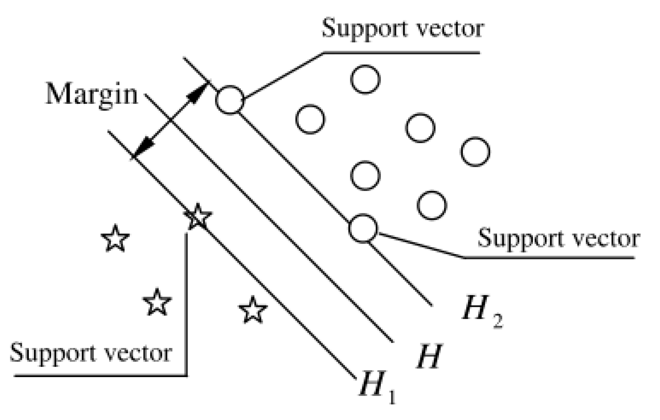
3.1. Support Vector Machine
3.1.1. SVM Theory
3.1.2. Multiclassification SVM
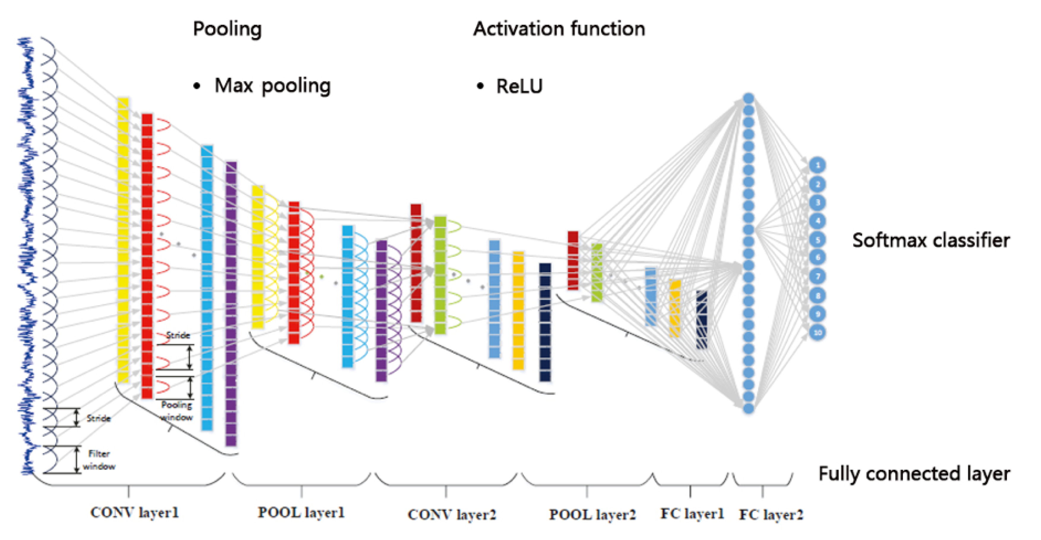
3.2. Convolutional Neural Network
3.2.1. Structure of CNN
3.2.2. Activation Function
- When the input is slightly away from the origin of coordinates, the gradient of the function becomes smaller—almost zero. During back propagation of neural network, the differential of each weight is calculated by the chain rule of differential. As back propagation passes through the sigmoid function, the differential on the chain is very small. Further, back propagation might pass through many sigmoid functions, finally resulting in little influence of weight on the loss function, which goes against weight optimization. This problem is called gradient saturation or gradient diffusion.
- If the function output is not centered on 0, the weight updating efficiency would decrease.
- The sigmoid function is applied in exponential operation, which is relatively slow for the computer.
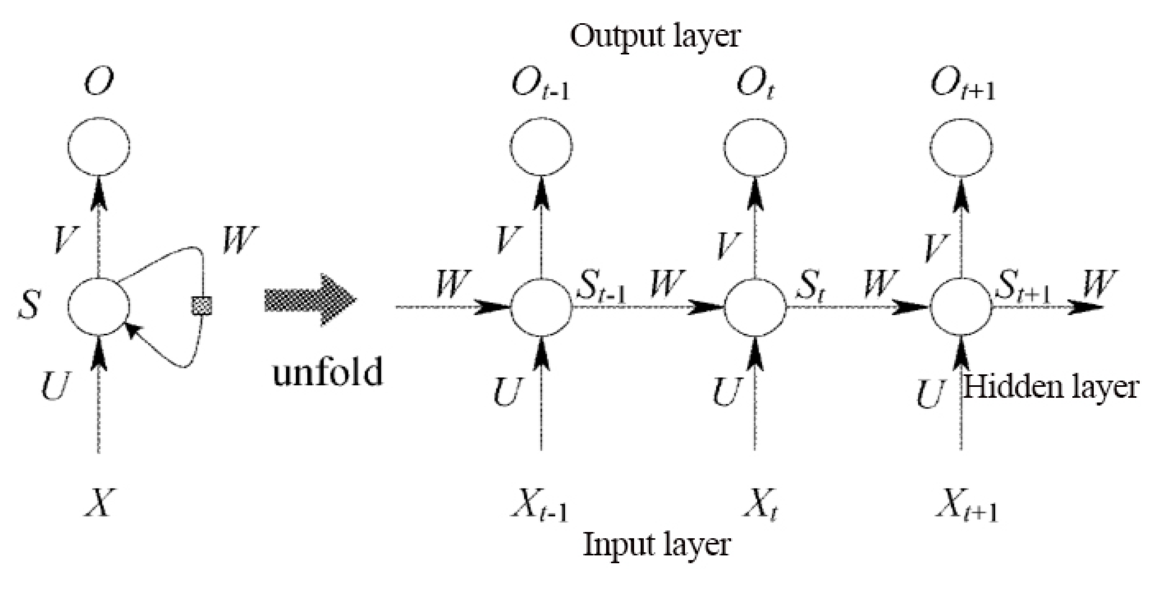
3.3. Long- and Short-Term Memory Neural Network Model
4. Example Verification and Comparison
4.1. Introduction of Data Source
4.2. Data Processing
4.3. Parameter Setting
4.4. Analysis of Results
4.4.1. SVM
4.4.2. CNN and LSTM
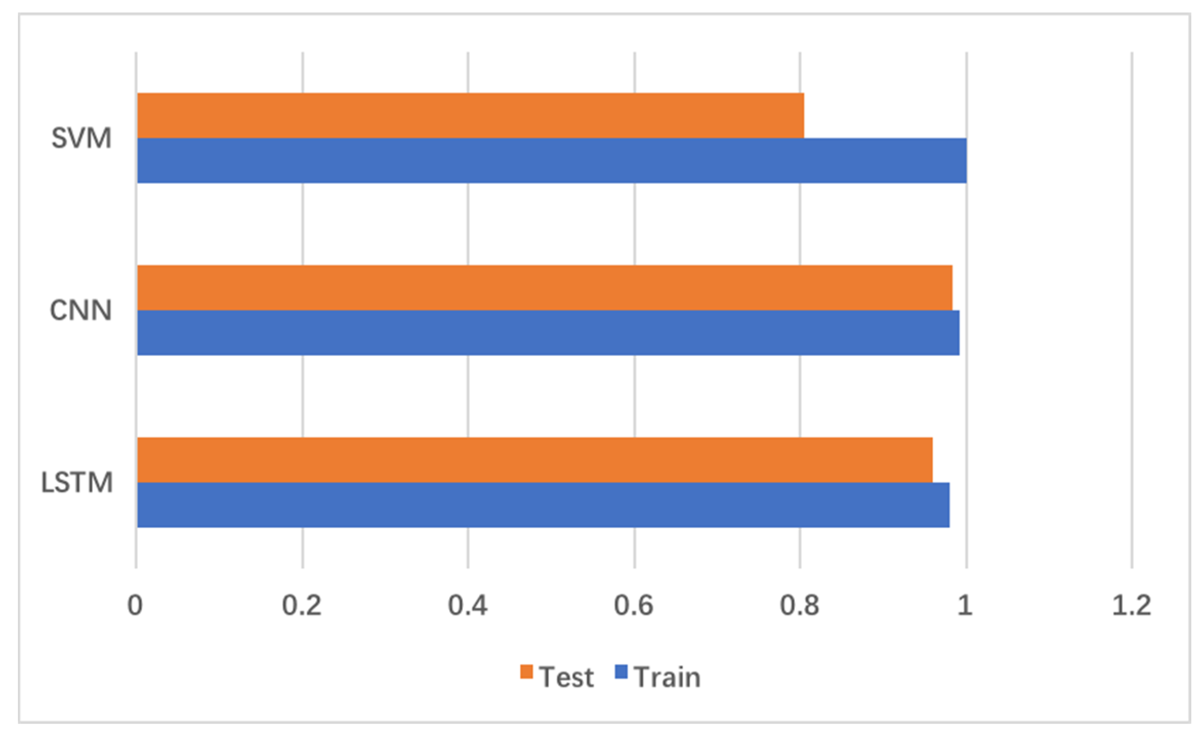
4.4.3. Comparison of Results
- Operation system: Windows 10, 64bit
- Central processing unit: I7-8750H@2.20GHz, 12-core
- Graphics processing unit: Nvidia Geforce GTX 1060max-Q (6 GB)
- Memory: DDR4-2666 8G+ DDR4-2666 4G
- Hard disk: KBG30ZMS128G NVME TOSHIBA
- Programming language and development environment: Python 3.6, Anaconda3-5.4.0
- Machine learning platform: TensorFlow 1.13.0
5. Conclusions
- The new method is better than the traditional and single statistical analysis method.
- For the classification of the time series fault data, the accuracy of the neural network is higher than that of the SVM.
- The CNN and LSTM both performed well. The CNN has slight superiority than LSTM regarding accuracy. More than that, LSTM is much more difficult to train. It takes much more time and requires higher equipment conditions. Generally, the CNN has greater advantages in the classification of the time series fault data than LSTM.
Supplementary Materials
Author Contributions
Funding
Conflicts of Interest
References
- Gomes, C.P. Computational sustainability: Computational methods for a sustainable environment, economy, and society. Bridge 2009, 39, 5–13. [Google Scholar]
- Frenkel, K.A. Computer science meets environmental science. Commun. ACM 2009, 52, 23. [Google Scholar] [CrossRef]
- Murgante, B.; Borruso, G.; Lapucci, A. Geocomputation, Sustainability and Environmental Planning; Springer-Verlag: Berlin, Germany, 2011; pp. 18–39. [Google Scholar]
- Hassani, H.; Huang, X.; Silva, E. Digitalisation and Big Data Mining in Banking. Big Data Cogn. Comput. 2018, 2, 18. [Google Scholar] [CrossRef]
- Hassani, H.; Huang, X.; Silva, E. Big-Crypto: Big Data, Blockchain and Cryptocurrency. Big Data Cogn. Comput. 2018, 2, 34. [Google Scholar] [CrossRef]
- Chen, M.; Yang, J.; Hao, Y.; Mao, S.; Hwang, K. A 5G cognitive system for healthcare. Big Data Cogn. Comput. 2017, 1, 2. [Google Scholar] [CrossRef]
- Chen, M.; Li, W.; Hao, Y.; Qian, Y.; Humar, I. Edge cognitive computing based smart healthcare system. Future Gener. Comput. Syst. 2018, 86, 403–411. [Google Scholar] [CrossRef]
- Steinhaeuser, K.; Chawla, N.V.; Ganguly, A.R. An exploration of climate data using complex networks. ACM Sigkdd Explor. Newsl. 2010, 12, 25. [Google Scholar] [CrossRef]
- Steinhaeuser, K.; Chawla, N.V.; Ganguly, A.R. Complex networks as a unified framework for descriptive analysis and predictive modeling in climate science. Stat. Anal. Data Min. 2011, 4, 497–511. [Google Scholar] [CrossRef]
- Lee, K.J.; Kahng, H.; Kim, S.B. Improving Environmental Sustainability by Characterizing Spatial and Temporal Concentrations of Ozone. Sustainability 2018, 10, 4551. [Google Scholar] [CrossRef]
- Hassani, H.; Huang, X.; Silva, E. Big Data and Climate Change. Big Data Cogn. Comput. 2019, 3, 12. [Google Scholar] [CrossRef]
- Anderson, R.P.; Dud, K.M.; Ferrier, S. Novel methods improve prediction of species’ distributions from occurrence data. Ecography 2006, 29, 129–151. [Google Scholar]
- Hastie, T.J.; Tibshirani, R.J.; Friedman, J.J.H. The Elements of Statistical Learning; Springer-Verlag: Berlin, Germany, 2009; pp. 56–97. [Google Scholar]
- Feng, X.; Li, Q.; Zhu, Y.; Hou, J.; Jin, L.; Wang, J. Artificial neural networks forecasting of PM 2.5 pollution using air mass trajectory based geographic model and wavelet transformation. Atmos. Environ. 2015, 107, 118–128. [Google Scholar] [CrossRef]
- Ekasingh, B.; Ngamsomsuke, K.; Letcher, R. A data mining approach to simulating farers’ crop choices for integrated water resources management. J. Environ. Manag. 2005, 77, 315–325. [Google Scholar] [CrossRef] [PubMed]
- Juan, R.P.; Emmanuel, L.; Juan, C.C.A. Estimating avocado sales using machine learning algorithms and weather data. Sustainability 2018, 10, 3498. [Google Scholar]
- Mazzoni, D.; Logan, J.; Diner, D. A data-mining approach to associating MISR smoke plume heights with MODIS fire measurements. Remote Sens. Environ. 2007, 107, 138–148. [Google Scholar] [CrossRef]
- Wang, L.; Zhao, Q.; Wen, Z. RAFFIA: Short-term Forest Fire Danger Rating Prediction via Multiclass Logistic Regression. Sustainability 2018, 10, 4620. [Google Scholar] [CrossRef]
- Zhang, J.; Wang, H. Looking at the development direction of aviation maintenance from the CMCS of Boeing 777. Aviat. Eng. Maint. 2000, 2, 25–36. [Google Scholar]
- Wang, B.K.; Chen, Y.F.; Liu, D.T.; Peng, X.Y. An embedded intelligent system for on-line anomaly detection of unmanned aerial vehicle. J. Intell. Fuzzy Syst. 2018, 34, 3535–3545. [Google Scholar] [CrossRef]
- Yuan, C.; Yao, H. Aeroengine intelligent performance diagnosis under sensor measurement deviation. Aviat. Dyn. Bull. 2007, 22, 126–131. [Google Scholar]
- Petrov, N.; Marinov, B.M. Methods for statistical valuation of the technical condition of aviation communication equipment. Acad. Open Internet J. 2000, 1, 133–147. [Google Scholar]
- Yang, Z. Research on Intelligent Fault Diagnosis Expert System for Aircraft Aviation and Electrical Equipment. Meas. Control Technol. 2006, 225, 4–7. [Google Scholar]
- Zhou, Y.; Cao, M. Application of Fuzzy Outward-Bound Fault Diagnosis in Aircraft Power System. J. Aviat. 1999, 20, 368–370. [Google Scholar]
- Bu, J.; Sun, R.; Bai, H.; Xu, R.; Xie, F.; Zhang, Y.; Ochieng, W.Y. Integrated method for the UAV navigation sensor anomaly detection. IET Radar Sonar Navig. 2017, 11, 847–853. [Google Scholar] [CrossRef]
- Fan, Z. Application of Kohonen Network in Engine Fault Diagnosis. Aviat. Dyn. Dly. 2000, 15, 89–92. [Google Scholar]
- Du, C. Fault Diagnosis Method of Avionics System Based on Rough Neural Network. Fire Power Command Control 2006, 31, 48–50. [Google Scholar]
- Xu, K.; Jiang, L. Aeroengine fault diagnosis based on Lyapunov exponential spectrum. J. Appl. Mech. 2006, 23, 488–492. [Google Scholar]
- Shi, R. Fault Diagnosis Expert System. J. Beijing Univ. Aeronaut. Astronaut. 1995, 21, 7–12. [Google Scholar]
- Baig, M.F.; Sayeed, N. Model-based reasoning for fault diagnosis of twin-spool turbofans. Proc. Inst. Mech. Eng. Part G J. Aerosp. Eng. 1998, 212, 109–116. [Google Scholar] [CrossRef]
- Palmer, K.A.; Bollas, G.M. Analysis of transient data in test designs for active fault detection and identification. Comput. Chem. Eng. 2019, 122, 93–104. [Google Scholar] [CrossRef]
- Kordestani, M.; Samadi, M.F.; Saif, M. A new fault diagnosis of multifunctional spoiler system using integrated artificial neural network and discrete wavelet transform methods. IEEE Sens. J. 2018, 18, 4990–5001. [Google Scholar] [CrossRef]
- Anami, B.S.; Pagi, V.B. Localisation of multiple faults in motorcycles based on the wavelet packet analysis of the produced sounds. IET Intell. Transp. Syst. 2013, 7, 296–304. [Google Scholar] [CrossRef]
- Chang, C.C.; Lin, C.J. LIBSVM: A library for support vector machines. ACM Trans. Internet Syst. Technol. 2011, 2, 1–27. [Google Scholar] [CrossRef]
- Hsu, C.W.; Lin, C.J. A comparison of methods for multiclass support vector machines. IEEE Trans. Neural Netw. 2002, 13, 415–425. [Google Scholar] [PubMed]
- Cristianini, N.; Shawe-Taylor, J. An Introduction to Support Vector Machines and Other Kernel-based Learning Methods; Cambridge University Press: Cambridge, UK, 2000; Available online: https://doi.org/10.1017/CBO9780511801389 (accessed on 2 July 2019).
- Vapnik, V.N. Statistical Learning Theory; John Wiley & Sons Inc.: New York, NY, USA, 1998; pp. 736–768. [Google Scholar]
- Kingma, D.P.; Ba, J. Adam: A method for stochastic optimization. In Proceedings of the 3rd International Conference on Learning Representations, (ICLR 2015), San Diego, CA, USA, 7 May 2015; p. 13. [Google Scholar]
- Vapnik, V.N. The Nature of Statistical Learning Theory; Springer: Berlin, Germany, 2005; pp. 878–887. [Google Scholar]
- Van, J.; Koc, M.; Lee, J. A prognostic algorithm for machine performance assessment and its application. Prod. Plan. Control 2004, 15, 796–801. [Google Scholar]
- Cortes, C.; Vapnik, V. Support-Vector Networks. Mach. Learn. 1995, 20, 273–297. [Google Scholar] [CrossRef]
- Hussain, S.F. A novel robust kernel for classifying high-dimensional data using Support Vector Machines. Expert Syst. Appl. 2019, 131, 116–131. [Google Scholar] [CrossRef]
- Noble, W.S. What is a support vector machine? Nat. Biotechnol. 2006, 24, 1565–1567. [Google Scholar] [CrossRef]
- Guo, Y.M.; Liu, Y.; Bakker, E.M.; Guo, Y.H.; Lew, M.S. CNN-RNN: A large-scale hierarchical image classification framework. Multimed. Tools Appl. 2018, 77, 10251–10271. [Google Scholar] [CrossRef]
- Felix, A.G.; Schmidhuber, J.; Cummins, F. Learning to Forget: Continual Prediction with LSTM. Neural Comput. 2000, 12, 2451–2471. [Google Scholar]


| Times | 1 | 2 | 3 | 4 | 5 | 6 | 7 | 8 | 9 | 10 | Average |
|---|---|---|---|---|---|---|---|---|---|---|---|
| F1-Score Training | 1 | 1 | 1 | 1 | 1 | 1 | 1 | 1 | 1 | 1 | 1 |
| F1-Score Test | 0.81 | 0.80 | 0.83 | 0.77 | 0.79 | 0.81 | 0.82 | 0.81 | 0.79 | 0.81 | 0.804 |
| Accuracy Test | 0.8 | 0.81 | 0.83 | 0.83 | 0.81 | 0.83 | 0.82 | 0.81 | 0.81 | 0.79 | 0.814 |
| Times | Accuracy | F1-Score | Loss |
|---|---|---|---|
| 1 | 0.975 | 0.989 |  |
| 2 | 0.9817 | 0.998 |  |
| 3 | 0.982 | 0.995 |  |
| 4 | 1.0 | 1.0 |  |
| 5 | 0.9817 | 0.986 |  |
| 6 | 0.9833 | 0.977 |  |
| 7 | 0.9834 | 0.997 |  |
| 8 | 1.0 | 1.0 | 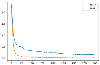 |
| 9 | 0.9843 | 0.988 |  |
| 10 | 0.9921 | 0.995 | 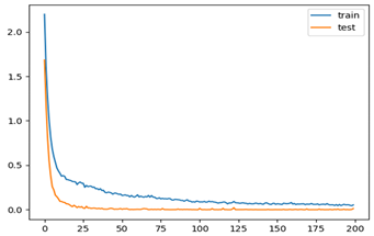 |
| Average | 0.9828 | 0.9925 |
| Val_acc of the Last 10 Iterations | Accuracy | Loss | F1-Score |
|---|---|---|---|
| 0.9733333388964335, 0.9466666777928671, 0.9333333373069763, 0.9900000095367432, 0.9933333396911621, 0.9900000095367432, 0.9733333388964335, 0.9900000095367432, 0.9900000095367432, 0.996666669845581 | 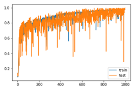 | 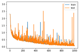 | 0.97 |
| Method | Training Time |
|---|---|
| SVM-RBF | 13.72 s |
| CNN epoch = 200 | 9 min 17 s |
| LSTM epoch = 1000 | 62 h 5 min |
| Data set | Precision | Recall | F1-Score |
|---|---|---|---|
| Train macro avg | 1.00 | 0.91 | 0.95 |
| Test macro avg | 0.75 | 0.12 | 0.21 |
| Training time | 3.2S | ||
© 2019 by the authors. Licensee MDPI, Basel, Switzerland. This article is an open access article distributed under the terms and conditions of the Creative Commons Attribution (CC BY) license (http://creativecommons.org/licenses/by/4.0/).
Share and Cite
Liu, C.; Jia, G. Industrial Big Data and Computational Sustainability: Multi-Method Comparison Driven by High-Dimensional Data for Improving Reliability and Sustainability of Complex Systems. Sustainability 2019, 11, 4557. https://doi.org/10.3390/su11174557
Liu C, Jia G. Industrial Big Data and Computational Sustainability: Multi-Method Comparison Driven by High-Dimensional Data for Improving Reliability and Sustainability of Complex Systems. Sustainability. 2019; 11(17):4557. https://doi.org/10.3390/su11174557
Chicago/Turabian StyleLiu, Chunting, and Guozhu Jia. 2019. "Industrial Big Data and Computational Sustainability: Multi-Method Comparison Driven by High-Dimensional Data for Improving Reliability and Sustainability of Complex Systems" Sustainability 11, no. 17: 4557. https://doi.org/10.3390/su11174557
APA StyleLiu, C., & Jia, G. (2019). Industrial Big Data and Computational Sustainability: Multi-Method Comparison Driven by High-Dimensional Data for Improving Reliability and Sustainability of Complex Systems. Sustainability, 11(17), 4557. https://doi.org/10.3390/su11174557