Article

Maximizing Environmental Impact Savings Potential through Innovative Biorefinery Alternatives: An Application of the TM-LCA Framework for Regional Scale Impact Assessment

1
Department of Management Engineering, Technical University of Denmark, 2800 Kgs. Lyngby, Denmark
2
Department of Plant and Environmental Science, University of Copenhagen, 1165 København, Denmark
3
Institute of Chemical Engineering, Biotechnology and Environmental Technology, The University of Southern Denmark, 5230 Odense, Denmark
*
Author to whom correspondence should be addressed.
Sustainability 2019, 11(14), 3836; https://doi.org/10.3390/su11143836
Submission received: 30 May 2019 / Revised: 9 July 2019 / Accepted: 11 July 2019 / Published: 13 July 2019

Abstract

:
In order to compare the maximum potential environmental impact savings that may result from the implementation of innovative biorefinery alternatives at a regional scale, the Territorial Metabolism-Life Cycle Assessment (TM-LCA) framework is implemented. With the goal of examining environmental impacts arising from technology-to-region (territory) compatibility, the framework is applied to two biorefinery alternatives, treating a mixture of cow manure and grape marc. The biorefineries produce either biogas alone or biogas and polyhydroxyalkanoates (PHA), a naturally occurring polymer. The production of PHA substitutes either polyethylene terephthalate (PET) or biosourced polylactide (PLA) production. The assessment is performed for two regions, one in Southern France and the other in Oregon, USA. Changing energy systems are taken into account via multiple dynamic energy provision scenarios. Territorial scale impacts are quantified using both LCA midpoint impact categories and single score indicators derived through multi-criteria decision assessment (MCDA). It is determined that in all probable future scenarios, a biorefinery with PHA-biogas co-production is preferable to a biorefinery only producing biogas. The TM-LCA framework facilitates the capture of technology and regionally specific impacts, such as impacts caused by local energy provision and potential impacts due to limitations in the availability of the defined feedstock leading to additional transport.

1. Introduction

Life cycle assessment (LCA) is a tool designed to quantify the environmental impact potential of products and services [1]. Recent advances in the field of LCA, such as the inclusion of temporal dynamism [2] and the coupling of LCA to urban metabolism [3] increase the applicability of the LCA methodology. Dynamism in LCA allows for the quantification of impacts while taking into consideration changing background and foreground systems, e.g., amounts of renewable and fossil energy sources in the electrical energy mix of a specific location in the background, and improvement to processing technologies in the foreground. On the other hand, coupling urban metabolism to LCA allows for large-scale assessments that better predict large-scale consequences of implementing a change at regional scale. These advances are an especially important input that can help guide the transition into a sustainable bioeconomy, as they allow for prospective studies. LCA of production systems/technologies, such as various agricultural productions, e.g., wine, cereal, and meat, can benefit from applying some of the new developments, since the large inputs and outputs to these systems, most likely, will have great environmental implications when changes to the production are implemented.
By applying the TM-LCA framework, as used in this study, it is possible to assess said systems in the specific context of the region, i.e., taking into consideration the region’s infrastructure, feedstock availability and accessibility, and the technical feasibility of technology implementation. Assessing large systems, as mentioned above, can be approached by defining the geographical boundaries in terms of a “producer territory” [4] so that the LCA can be applied for assessment of a delimited “territory”, e.g., wine-producing areas, within a broadly defined region, e.g., Southern France. The producer territory is thus defined as the area of interaction between the aggregated producers and other systems within the region. The TM-LCA framework reduces data demand by aggregating individual areas of the production of, for example, a specific product, supply chain or waste treatment technology, while ignoring unchanging background systems, i.e., only changes to the region interacting with the producer territory are assessed. At the same time, representativeness is increased by merging local inventory data from individual producers with regional and nation-wide data in order to fill in data gaps. In this way, an environmental performance improvement in the territory, due to, e.g., the implementation of a new technology or new management technique, can be quantified in the non-contiguous production area and is reflected in the results for the region. When combined with dynamic and prospective LCA [2], this approach offers a comprehensive assessment that gives temporally and geographically resolved results. Moreover, it has the added utility of providing prospective insights that can more accurately support decision makers, production owners, and technology developers [4].
A point of departure for many LCAs is a static product system, where, for example, technology A might be assessed against technology B for the making of a product. The static nature of LCA is problematic when applied to products or systems with long service lives [5], due to inconsistencies in time horizons and changes in background systems [6,7]. Previous work has demonstrated the importance of incorporating various types of dynamism into LCA, as this can significantly affect the results of the study [6]. In this regard, it is possible to add dynamism to the various stages of the LCA in a consistent, systematic, and transparent manner, as outlined in [2] and shown in various other publications [7,8,9]. Following the TM-LCA framework, dynamism can be added in a consistent manner from the start, which provides added information regarding the sensitivity of the system to background changes. Real production systems are rarely static, and results based on static systems can sometimes exhibit rank reversal when compared to dynamic results [10]. Thus, basing future decisions on static LCAs can result in building significant error into the models and associated results. Adding dynamic aspects to LCAs can increase the analytical accuracy of results [11].
The added layers of information to the TM-LCA mean that the interpretation phase becomes more resource demanding. This can be eased by the use of extra tools, such as multi-criteria decision assessment (MCDA). Midpoint results for 18 different impact categories of an LCA are often difficult and time consuming to synthesize into clear and readily applicable decision support. When adding dynamism, this translates into temporally specific results for, e.g., each year of the time horizon, for each of the 18 impact categories. Out of the many MCDA methods that exist, one that has shown great capability in dealing with LCA results is Technique for Order of Preference by Similarity to Ideal Solution (TOPSIS) [12,13]. The output from TOPSIS is given in the form of a single score performance index, which is used to derive preference between the scenarios being assessed. By checking a multiple criteria decision support tool used with equal weightings for all midpoint impact categories, it is easy to realize and visualize burden shifting amongst the midpoint impact categories, when used in conjunction with a visual inspection of internally normalized results. The MCDA approach is considered preferable, as using carbon footprint alone has been shown to give potentially misleading results [14].
The present study’s goal is to implement an assessment based on the TM-LCA approach [4] in order to provide a comparison of potential biorefinery choices for the treatment of agricultural residues. For the demonstration of TM-LCA, a biogas production scenario is compared to a scenario of combined biogas and Polyhydroxyalkanoates (PHA) production, which is currently being developed at pilot scale. Polyhydroxyalkanoates are naturally occurring polymers produced by a consortium of bacteria, which can feed on the volatile fatty acid (VFA) stream generated by the acidogenic phase of anaerobic digestion (AD) [15]. PHA, which is also found as polyhydroxybutyrate (PHB), can be used to produce biodegradable plastic products. In this case, PHB production substitutes the production of polyethylene terephthalate (PET) or polylactide (PLA). The two biorefinery scenarios are modeled with dynamics built into both foreground and background systems. In the foreground system, dynamics are included as a yearly decrease in the amount of energy consumption needed to produce PHA. In the background system, the electrical energy mix, hereafter referred to as energy mix or energy grid, of both locations is varied yearly for a period of 20 years with four possible provision mixes for Oregon, and five possible choices of provision for the energy mix futures of France. The scenarios are then tested at a territorial scale as described above, i.e., processing all the feedstock in the region in the two geographically dissimilar production territories, to observe the effects of regional differences on territorial performance. Since the use of global warming potential (GWP) as a single indicator has been shown to provide potentially misleading results [14], MCDA is applied in the interpretation phase to help ease the interpretation of results.

2. Materials and Methods

2.1. TM-LCA Framework Application

The application of the TM-LCA framework is described in general terms here. A point of departure for the application of the TM-LCA framework is the functional unit. The functional unit, the treatment of one ton of feedstock of specific composition, is treated by two different technology alternatives, described in more detail below. From here, the following steps are applied and described through the methodology:
(a)
Alternative technology is defined.
(b)
The producer territory is defined and limited to systems interacting with the technological options being assessed within a geographical region.
(c)
Temporal dynamics are incorporated into the systems, e.g., in dynamic background electricity energy provision and technological efficiency improvement.
(d)
The assessment is scaled to encompass the whole region so that all feedstock available that may fulfill the functional unit is treated by the technological alternatives being assessed. However, only changes in systems and in the region are assessed.

2.2. Goal and Scope

In order to implement the TM-LCA framework, two options for the treatment of agricultural residues were modelled and compared in two geographic locations, the Languedoc-Roussillon region in southeast France and the Willamette, Umpqua, Rogue, and Columbia valleys of Oregon State in the USA. Advancements in biogas technology make it possible to treat a plethora of agricultural residues, and recent innovation allows for the production of value-added products, in this case, the family of biopolymers known as polyhydroxyalkanoates (PHA). This innovative technology, which effectively creates a biogas platform for new biorefineries, is a contender to conventional biogas production where the only products are biogas and digestate. The proliferation of biogas plants makes this new addition to anaerobic digestion a highly transferable technology, which can be implemented wherever agricultural residues are available. Since biorefineries, in general, have a long service life (decades) and draw from large discontiguous areas, both territorial and dynamic aspects of this assessment are an advantage for decision makers considering biorefinery options for their region. However, it should be emphasized that the study only compares two different biorefinery types. It cannot be used to decide whether to increase the total use of residues for biorefineries.

Functional Unit

The basis for the comparison of the scenarios is the treatment of 1000 kg of feedstock. The feedstock is assumed to be agricultural residues of the following composition: 50% liquid cow manure, 15% solid cow manure, and 35% wine pomace or wine marc, hereafter used interchangeably. Feedstock characterization is based on laboratory tests performed onsite at an Italian biogas plant for the liquid and solid manure, while for wine pomace it is based on literature values. While other types of feedstock can be treated by the biorefineries being considered, the choice of feedstock was limited to the above in order to better appreciate the difference between biorefineries rather than differences arising from choice of feedstock. The feedstock physiochemical properties are presented in the supplementary information (SI).

2.3. Scenarios

Two baseline scenarios were assessed with the OpenLCA [16] software and the Ecoinvent 3.4 database [17]. The two alternative technological pathways possible for treating the functional unit are:

2.3.1. Biogas Only

Conventional biogas production was modelled as the anaerobic digestion step of biogas production, which produces biogas and digestate. The biogas was assumed to be burned in a combined heat and power (CHP) engine, producing electricity and heat based on the energy content of the biogas. Process energy consumption was calculated to be 7% of the electricity output, based on data received from an industrial scale biogas plant in Northern Italy, while the co-generated heat is assumed to be wasted. This is due to the geographical areas of implementation of the scenarios, where the excess heat is not used. Furthermore, adding the produced heat to this study would only change the magnitude of the savings from displaced energy production, and not the ranking of the scenarios, as seen in [18], as the magnitude of heat production is similar across scenarios. All other operational parameters were also based on the data acquired from the abovementioned biogas plant and are available in the supplementary information (SI).
Processing steps that are equal for both scenarios and emissions occurring therein, e.g., feedstock storage, animal housing and digestate storage, were excluded from the assessment, as they would result in no relative difference. Similarly, phosphorus fertilizer replacement was left out because the starting content of P is the same, and processing is not expected to change this. Adding replacement of P fertilizer to the assessment would only elucidate differences between digestate and mineral fertilizers, which is not the focus of this study.

2.3.2. Field Application of Digestate for All Scenarios

The field application of the digestate was modelled, and conventional ammonium nitrate fertilizer was assumed to be replaced. It is well known that digestates mineralize at a slower rate so that a share of the organic nitrogen present in digestate will be bound and will thereby not be available for crop uptake or emissions. Thus, an average mineral fertilizer equivalency value of 67.5%, calculated from a review of values that are commonly used in this type of assessment, was used for the substitution of mineral N fertilizer [19]. Emissions resulting from the field application of digestate were modeled based on the approach in [20], which applied the agronomic model Daisy [21] to estimate long-term emissions from different types of soils with different histories of management, i.e., high or low inputs of organic matter in the form of organic fertilizers, such as digestate and compost. As shown in this work, the crop’s response to nutrient inputs is highly dependent on the previous fertilization history of the field. Emission factors (EFs) for high and low crop response after digestate application were taken from [22], which follows the same approach described by [20] and had soils and overall conditions which more or less match the soils in the geographical areas assessed here. For N2O emissions, the Intergovernmental Panel on Climate Change (IPCC) methodology [23] and EFs were used. The sensitivity of N2O EFs was tested in the sensitivity analysis due to the multiple models available for deriving EFs. The nutrient content of the digestates, as well as emission factors for all N-related emissions, for digestates and mineral N fertilizer are presented in Supplementary Tables S1, S2 and S4.

2.3.3. PHA-Biogas

The second scenario represents a tweaking to the AD process, where AD is split so that the VFA production that occurs during the first days of digestion is diverted and used to produce and feed biomass capable of producing PHA. Operational data from a PHA-producing pilot plant run by Innoven Srl were obtained and used to create an industrial scale model of PHA production. The co-production of biogas and PHA is executed, albeit with a lower biogas yield. Just as above, digestate continues to be produced and replaces mineral N fertilizer. Additionally, the extraction of polyhydroxybutyrate (PHB), a polymer in the family of polyhydroxyalkanoates, i.e., PHAs, is included as the addition of process energy consumption for the extraction, and hydrogen peroxide is included as an extraction agent. All other model parameters are equal to the biogas scenario.
PHA production is here assumed to be 100% PHB and replaces the production of petroleum or bio-based polymers, referred to as the replacement polymers (RP). In the first run of the model, PHB replaces PET at the factory gate, with a replacement ratio of 0.93:1 PHB to PET. In terms of material properties, several performance indices (PI) based on yield strength (σ), tensile strength, and density (ρ) were used to derive the replacement ratios (RR) (Equation (1)). The ratio of replacement is tested in the sensitivity analysis so as to represent different applications of the polymer more accurately. The choice of polymer substitution is also tested; since PHA is a bio-sourced biopolymer, a sub-scenario with replacement of biobased polylactide (PLA) is also presented. The RR is 0.64 for PHB substitution of PLA, based on Equation (1).
R R = P I P H B P I R P ,   and   P I = σ ρ
Equation (1) Polymer replacement ratio, where RR = replacement ratio, PI = performance index, σ = yield strength, RP = replacement polymer and ρ = density.
The addition of PHA production in this scenario is not burden-free, inducing impacts from energy consumption and via the production of the extraction agent. However, due to missing data from the pilot plant, the additional energy consumption was calculated using the process design software Superpro Designer® [24]. This yields an additional 7 kwh/functional unit (FU). It was assumed that process energy consumption for PHA could improve over time, so a 1% decrease in energy demand per year for PHA production was modeled for the assessed period. This represents the maturation of PHA extraction technology, which is a likely scenario as the implementation of PHA extraction in biorefineries becomes more widespread and further optimization of the technology takes place. This efficiency improvement rate is tested in the sensitivity analysis to explore the possibility of faster and slower improvements to the process. Key parameters for the production of PHB are presented in Supplementary Table S3.

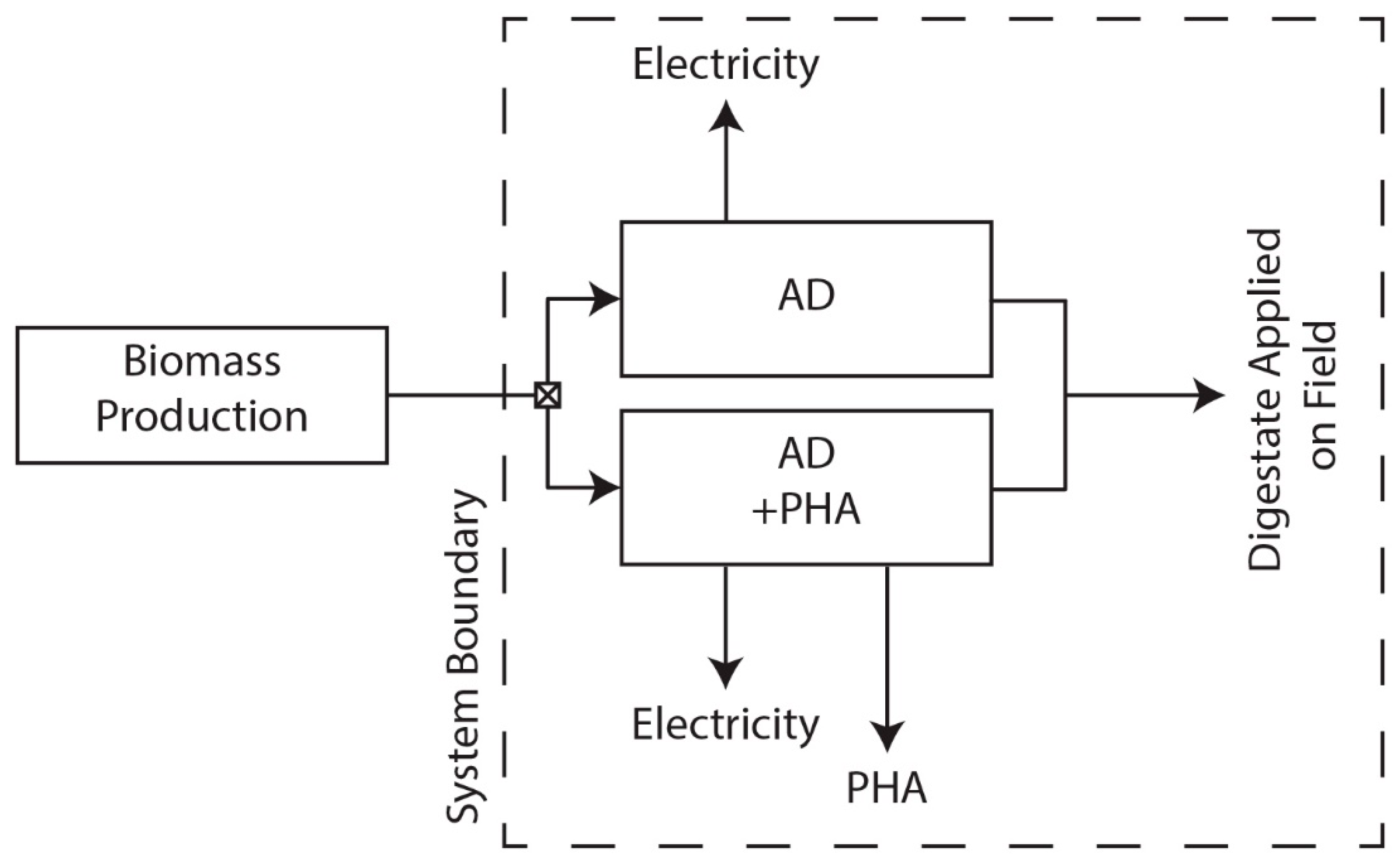
2.3.4. System Boundaries

The system boundary of the two scenarios extends from when the feedstock enters AD to the application of digestate onto the field (see Figure 1). End of life was not included in the assessment, as the LCA methodology lacks an appropriate characterization of the effects from plastic degradation in the environment, such as microplastic formation and the production of methane among other decomposition gases [25,26].
Applying a dynamic approach, all background and foreground processes were modified so that the two geographical areas are accurately represented with likely different future energy production scenarios in accordance with the national and state-specific energy legislations and policies.

2.4. Dynamics

Dynamic inventories of the electricity mix for the two locations, modelled for a period of 20 years from 2015–2035, were used in the analysis. Four different dynamic energy futures, developed by the French government, with yearly shifting percentages of contributing sources of energy (Figure 2), were used for all electricity provision in the scenarios for Languedoc-Roussillon [27]. Likewise, three different dynamic energy futures were developed based on the legislation for Oregon State (Figure 3), which regulates the share of renewables in Oregon’s future energy grid [28]. Qualifying renewables, i.e., renewable energy sources accepted by Oregon legislation on renewables, were introduced in varying amounts. Thus, (1) a scenario where biomass was increased more than other qualifying renewables, (2) a scenario where wind and solar were increased more than other qualifying renewables, and (3) a scenario where all qualifying renewables were increased evenly were developed. Static electricity mix scenarios were also included for both locations.
To maintain consistency in the foreground and background systems, the electricity provision component of all Ecoinvent processes used in the assessment was exchanged with the dynamic mixes developed. This included the electricity for fertilizer production, conventional polymer production, and the electricity replaced in the grid. This use of the local grid mix in the commodity production may not be a 100% accurate representation of a market reaction for the background systems, but it is deemed a better representation than the static processes. Further discussion on this subject can be found in Section 4.

PHA Process Energy Consumption

PHA production, which has been around since the 1980s, is already practiced at industrial level with first generation feedstock such as sugars from corn and sugarcane. Plants already exist with capacities ranging from 2000 to 50,000 tons of annual production [29]. Furthermore, PHA production has been introduced to the waste water treatment sector [30,31] and is also possible from second generation biomass. Due to important experience in the market with regards to PHA production, the PHA production for second generation biomass, as in the present study, will likely attain vast improvements in the future, eventually reaching a maturity level comparable to current industrial PHA production. To reflect this, dynamics in the PHA inventory were included in terms of electricity consumption (i.e., energy efficiency), in addition to the dynamic electricity provision. Hence, while PHA production was modelled starting as 7 kwh/FU more burdensome than the biogas-only scenario, thereafter the process was modelled as becoming more energy efficient, improving by 1% annually for the 20-year period, based on similar technology learning curves [32]. This improvement rate was also tested in terms of influence on total impacts (see Section 2.7).

2.5. Implementation of Territorial Scale Assessment

In order to assess the implications of implementing PHA technology at a territorial scale, the two study regions, in France and Oregon respectively, were analyzed regarding ability to provide feedstock for application in the two assessed biorefinery scenarios, i.e., impacts arising from treating all feedstock available in the region by biogas-only or combined PHA-biogas. The territories were defined as the interacting areas of residue production and the treatment plants. However, as defined in the TM-LCA method [4], only the areas undergoing change are included in the assessment. In this case, the change is an average change reflected in the residue treatment centers. Therefore, it is not expected that this change will affect the production of the residues in any way, ergo feedstock producers are left out of the assessment in terms of environmental impact. Likewise, transport from producers to treatment centers is not expected to change, as the volume of residues produced will not change as a consequence of implementing PHA technology. Where there is potential for transport that would deviate from the status quo, namely in the transport of grape marc which is the lighter of the two feedstock, impacts from transport were assessed (see 0, Sensitivity Analysis). These impacts were not included in the main results, as the induced impacts from transport would be equal in both the PHA-biogas and the biogas-only scenarios.

Feedstock Provision

Several assumptions were made in relation to determining the amounts of residue produced in each region for input into the regional scale assessment (Table 1). For wineries, it is assumed that grape marc is produced at a rate of 0.13 tons per ton of processed wine grapes [33]. It is further assumed that in France, where production data are reported in hectoliters of wine instead of mass of grapes at crush, 140 kg of grapes are used to produce 1 hectoliter of wine [34]. For feedstock coming from cattle, it is assumed that all waste comes from dairy cattle and that dairy cattle produce waste at a rate of 54.5 kg per head per day [35].
Due to the relative scale of wine production and the cattle industry in Oregon, the production capacity of the biorefinery systems in Oregon is limited by the production of grape marc, assuming that the co-digestion of cow waste and grape marc is not augmented with alternative feedstock. With nearly 2.4 million tons of waste produced by dairy cattle annually [35] and only 8010 tons of grape marc produced annually, the treatment of all grape marc (at 35% of total treated biomass) would require appx. 1% of the dairy cattle manure provision capability of Oregon. However, the total production of this system might not be enough to provision a fully industrial scale biogas plant, though it would be enough to provision a smaller scale plant, and implications of this are discussed in Section 2.7.4.
Conversely, in relation to Oregon, the capacity of the biorefinery systems in Languedoc-Roussillon is limited by the production of manure. With only 18,700 dairy cattle [36], the region would only be able to supply appx. 0.37 million tons of the 0.39 million tons manure needed for co-digestion with the 0.21 million tons of grape marc produced in the region annually (CIVL—Conseil Interprofessionnel des vin AOC du Languedoc et des IGP Sud de France—Languedoc Wines). This relationship, unlike that in Oregon, is fairly well balanced. However, unlike in Oregon, there are well-established uses for grape marc, so the ability to provide grape marc as feedstock would therefore compete with existing demand (see Section 4).

2.6. Impact Assessment Method

The ReCiPe 2016 Hierarchist method was used for impact assessment [37]. Impacts were assessed at the midpoint level with a time horizon of 100 years from the time of emission. All impact categories were included in the assessment of the dynamic system model and in all scenarios.
While all impact categories were modelled, using all indicators creates difficulty in relation to the interpretation of the results. To avoid this obstacle, GWP was chosen as a single indicator for impacts. In order to check for potential burden shifting when solely using GWP as an indicator impact, TOPSIS was applied with equal weighting to all impact categories. Ranking of the scenario results was then performed in a pairwise fashion, i.e., within each energy mix future, for the two scenarios, biogas-only and PHA-biogas, using both GWP as a single score indicator and TOPSIS.

2.7. Sensitivity Analysis

Important modelling parameters and assumptions were tested through a sensitivity analysis. These include:

2.7.1. Process Energy Consumption Related to PHA Production

Energy consumption related to PHB production was calculated using process design software, and it was subsequently tested to see if the overall results were sensitive to this parameter. Thus, a scenario where the energy consumption of PHB production does not improve over time was tested. For contrast, a scenario where processing improves by 5% per year was also explored.

2.7.2. Replacement Ratio Conventional Polymers

Replacement ratios of PHB to PET and PLA were estimated using the following material property indices: tensile strength, yield strength (σ), and the average between tensile strength and yield strength. RRs in the first model run were based on yield strength (σ), which applies to brittle polymers that are loaded in tension. This is done in order to relate the polymer matrix to its final application, which is unknown and is most likely several different applications for this case study. Thus, by choosing a handful of material properties, it is possible to estimate more realistic RRs that apply to desired properties. The values used of the RR estimation are presented in Table 2.

2.7.3. Mineralization of N in Digestate

An important source of uncertainty comes from the application of digestate to the field. In the first model run, EFs for N2O emissions were based on IPCC values. To test the possible range of impact arising from N2O emissions in the field, a powerful greenhouse gas, a second model run was performed using the N2O emission factors published by [22]. Though these are not local EFs, they are used to portray the potential variation of greenhouse gas emissions after digestate application. The values used are found in Supplementary Table S5.

2.7.4. Feedstock Provisioning Scenarios

In both regions, there is potential for increased ground transportation induced by transport of grape marc for PHB production. Transport for grape marc is, in most cases, non-existent in Oregon whereas transport is used to distribute grape marc amongst various end-users in France. This means that implementing a PHA-producing biorefinery would either route or re-route the grape marc needed as feedstock to the biorefinery. To account for this, the system was modelled with ground transport of the grape marc by lorry. This was done for various potential transport distances ranging from 50–500 km for the PET replacement scenario.

3. Results

Results showed that the PHA scenarios outperformed the biogas-only scenarios in almost every impact category with a few exceptions (Figure 4). Exceptions included the French energy scenarios for the Ionizing Radiation (IR) impact category and almost all scenarios for Land Use (LU), except in one instance, the Oregon Static scenario, where PHA-biogas performed better than biogas-only in terms of LU.
It is worth noting that in some of the impact categories the difference between the two scenarios is so small that, keeping in mind the considerable uncertainty of LCA results in general, it is fair to say that both PHA-biogas and biogas-only are essentially equal in terms of environmental impact. This is true for the Particulate Matter (PM), Fresh Water Ecotoxicity (FWE), Land Use (LU), Marine Ecotoxicity (MEtox), Marine Eutrophication (ME), Mineral Resource Scarcity (MRC), both Ozone Formation categories, Terrestrial Acidification (TA), and Stratospheric Ozone Depletion (SOD) impact categories. The remaining impact categories show a greater degree of difference, where it is clear that the PHA scenarios are generally preferable. Midpoint impact category results are presented as percent reduction in environmental impact from the implementation of PHA production in relation to biogas-only scenarios, for all energy provision scenarios. These are shown both for scenarios replacing PET with a ca. 93% RR and a 30% RR, to show the influence of RR in impact results (Figure 5).
The first model run shown in Figure 4 has PET as the conventional polymer to be replaced by PHB. The model was checked to see if a different polymer substitution material would alter the results. It was found that a change to PLA as the polymer substitution material did not change the general ranking, but the magnitude of the difference between PHA-biogas and biogas-only, i.e., the advantage that PHA-biogas has over biogas-only, decreased. Figures and tables for the PHA-biogas results for PLA are shown in the SI (Supplementary Figure S4 and Table S7).
Figure 6 shows the difference between the PHA-biogas and biogas-only scenarios, i.e., PHA-biogas CO2-eq minus biogas-only, in CO2-eq. For all 20 years, the PHA-biogas scenario induces greater savings than the biogas-only scenarios, which is why the results are always negative. Furthermore, the general negative slope of all scenario lines shows that as time progresses PHA-biogas becomes more attractive, inducing higher savings in comparison to biogas-only. More interestingly, it is possible to observe the difference between plans for energy grid development in the two locations. Hence, Oregon scenarios show a steeper slope, i.e., a drastic pull back from the use of fossil fuels and, more specifically, the use of coal. In contrast, the French slopes are less pronounced, as improvements to the grid are subtler because there is already a large share of non-fossil-based energy production in use in France. The difference between the two regions is larger at the beginning of the period, getting smaller in time as the grids progressively increase their share of renewable energy.

3.1. Sensitivity Results

The robustness of model results was checked by varying different parameters, as described in the methodology, Section 2.7. After each change, indicators were checked with the TOPSIS and GWP single indicators, but for the most part, there was no change to the preference ranking of the scenarios, and combined PHA-biogas production continued to perform better. Thus, it can be said that the model results are robust in regards to the most influential parameters analyzed.
In more detail, changes to the replacement ratio (RR), i.e., the PHB: PET mass ratio that is allowed by different material properties, as discussed in Section 2.7.2, was shown to be a moderately sensitive parameter. A 5% change in the replacement ratio lead to a 3–4% change in results for PHA-biogas with PET (Figure 7), and a 2.5–4% change in results for PHA-biogas with PLA. Thus, it can be said that a general trend is observed of lower savings with lower RR (or higher savings with higher RR), while the effect of the change is nearly proportional to the change seen in the results.
The sensitivity to efficiency improvements for PHA-producing technology was also tested and it is shown in the SI, Figure S3. This parameter was showed to have very little effect on overall model results, with GWP changing in the range of 0.1–1.5%.

Sensitivity of N2O Emission Factor

Cumulative global warming impacts switch from a savings inducing status to a burden inducing status when N2O emission factors for the field application of digestate from [22] are applied (Supplementary Figure S4). However, the ranking between PHA-biogas and biogas-only stays the same, with combined PHA-biogas scenarios continuing to perform better than biogas-only scenarios. The results show that N2O emissions play an important role, and considering the strong dependency on local conditions, they should as much as possible be spatially differentiated. The variability of N2O emissions for the EFs employed can be seen in Figure 8.

3.2. Territorial Scale Application

Application of the biorefinery alternatives at a territorial scale would lead to potential reductions in regional environmental impact. In order to give a measure of scale to the potential savings induced by the implementation of maximum (limited by feedstock availability) PHA-biogas production relative to biogas-only, the GWP impacts were normalized using planetary boundary carrying capacity-based normalization factors [41]. Assuming a 985 kg CO2 eq. per person year (PY) carrying capacity (C.Cap) [41], and assuming that PHA replaces PET with a 93% RR and that the PHA process improves in terms of energy efficiency at 1% annually, the production of PHA induces an average reduction in GWP impacts relative to biogas-only equating to nearly 1400 PY of C.Cap. When broken down by region, the French scenarios indicate an average relative maximum potential GWP saving of over 2400 PY of C.Cap, with Oregon exhibiting just over 80 PY of C.Cap in average relative maximum potential GWP savings. Using the same assumptions, except exchanging the replacement polymer with PLA production at a 64% RR, then the maximum implementation in France and Oregon of the PHA-biogas scenario induces an average annual potential relative GWP impact reduction of 493 PY of C.Cap when compared to production of biogas-only, with 871 and 21 PY of C.Cap in France and Oregon, respectively, see Table 3.

Sensitivity Analysis of Transport at Territorial Scale

The importance of transport was tested via sensitivity analysis of different theoretical grape marc transport distances for both the biogas-only and PHA-biogas scenarios (Table 4). For all scenarios, a 500 km transport distance results in overall elimination of environmental benefits, and at 200 km, transport of grape marc reduces average impact savings from the various biorefinery-region scenarios by 42.5% for all midpoint indicators. In terms of GWP, a 200 km transport distance induces impacts of a maximum of appx. 284% and a minimum of 68% of the magnitude of GWP savings without transport. At 50 km, all scenarios show reductions in GWP. At 100 km, all PHA production scenarios and France biogas-only scenarios induce GWP savings, while the Oregon biogas-only production scenarios eliminate the GWP benefit of implementing the biorefinery. Furthermore, if the introduction of centralized PHA-Biogas biorefineries were to induce transport of grape marc, relative to existing decentralized biogas production, then GWP savings are overwhelmed by the induced impact from transportation at any distance greater than appx. 125 km.

4. Discussion

Overall, the model results obtained were robust and indicate that implementing PHA production technology is preferable to conventional anaerobic digestion, when the functional unit (FU) equals 1 ton of feedstock treated. Combined PHA-biogas scenarios, whether with PET or PLA as the replaced polymer, performed better across almost every impact category. This is largely due to the added benefit of replacing conventional polymers, which are associated with significant impacts. As evidenced by the replacement ratio (RR) sensitivity analysis, decreasing or increasing the amount of PHB needed to equate the function of PET or PLA resulted in an almost proportional effect in the outcome. RR of PET would have to decrease by around 80% and be as low as 20% before there is rank reversal between the two options in some of the impact categories. This was confirmed by both single score indicators, which prefer combined PHA-biogas scenarios until reaching values close to 20% RR (Table 5). However, the GWP single indicator still preferred PHA-biogas, even at a 20% RR, except for the OR-Static Scenario. On the contrary, the TOPSIS single indicator, which is equally weighted between impact categories, starts preferring biogas-only scenarios earlier, with a 35% RR. In this regard, there was less operating space for the GWP indicator, when PLA is the replacement polymer, which starts signaling biogas-only as the preferred choice already at 30% RR. On the contrary, TOPSIS selects biogas-only at low RR of 9–16%. Thus, there is disagreement between the GWP and TOPSIS single indicators, which is, furthermore, replacement polymer-dependent. This points to two issues to consider: (1) choosing GWP as the only impact category for the assessment can potentially result in burden shifting to other environmental impact categories and (2) the choice of polymer substitution affects impact categories other than GWP, here exemplified by the difference in the TOPSIS results when choosing PET or PLA as polymer replacement. To elaborate, the difference lies in PET’s production being more burdensome for impact categories other than GWP in comparison to PLA’s production. However, the single score indicators employed generally indicated a similar scenario prioritization, i.e., combined PHA-biogas production being the preferred choice across all future energy scenarios, as long as RRs were higher than 20% for PET and 30% for PLA. It is worth noting that such a low replacement ratio is considered unrealistic, as the material properties of PHB allow for various applications [40].
Much like with polymer replacement ratios, TOPSIS and GWP do not always agree when the limits of process energy consumption are tested. If process energy consumption reaches 134 kWh per FU of added energy demand for PHA production, then TOPSIS (unlike GWP) indicates preference for biogas-only, for all energy scenarios, which indicates there is a potential for burden shifting if GWP is chosen as the only indicator. However, unlike the replacement ratio, improvements in process energy consumption for the production of PHA lead to very small changes in results. If there is no improvement in process energy consumption, meaning production of PHA consumes 7 kWh more per FU than the biogas-only scenario, results still stay the same. The break-even point of energy consumption for PHA production is high, i.e., it takes 12 times this value, 85 kWh of added process energy consumption of PHA per ton feedstock, before the TOPSIS-derived single indicator shows preference for biogas-only over combined PHA-biogas production for several of the French energy scenarios and one Oregon scenario. Moreover, it takes 16 times this value, or 113 kWh/FU more, before it is possible to observe prioritization change for the GWP single indicator for one Oregon scenario, the OR-Static Scenario, and 32 times the initial value, 226kWh/FU, before all Oregon energy scenarios show a preference for biogas-only. As for France, it is not until PHA production consumes 55 times this value, 389 kWh/FU, before there is a change in the GWP single indicator in preference of one of the energy future scenarios; the FR-Static Scenario. Thus, it is possible to conclude that there is large leeway in process energy consumption for PHA production before the decision support will change, in terms of GWP. As exemplified here, this is also dependent on the share of renewable energy sources in the future energy grid, which is why results are more robust for France in terms of GWP, i.e., requiring 55 times, 7 kWh/FU, more energy consumption before seeing a change in GWP impact category. The energy prediction mix is thereby an important factor when deriving the impacts of the system, which are heavily affected by energy mix usage.
In this regard, using dynamic energy grids for the background is a powerful tool. Many nuances are highlighted and originate from the predicted/expected changes in the share of renewable energy for the different locations. The most obvious of these subtleties can be observed in the Ionizing Radiation category (Figure 4), where it is evident that there is a higher share of nuclear energy in the French background system than in that of Oregon. As seen in Figure 6, the evolution of the energy grid reveals a sharp decrease for Oregon, while France’s energy grid remains somewhat unaltered. This is due to legal requirements in Oregon, which are intended to increase the share of renewables from 15% to 50% by 2040 [28]. Greening of the energy grids increases the difference between biogas-only and PHA-biogas in the future, as is exhibited by the negative slopes of the lines in Figure 6. Despite the increasing environmental importance of plastic replacement as opposed to electricity replacement, it is worth restating that PHA-biogas is consistently preferable in terms of GWP, i.e., negative values throughout the assessment period. One major area discussion regarding the dynamic inventory is the use of local energy mix scenarios in commodity replacement. It is likely that the increased production of PHA would have no direct effect on the production of PET or PLA in Oregon or France. However, by using a local instead of global process, it is possible to develop processes that are treated equally, in terms of system dynamism, for their inventory development. Furthermore, this is seen as a cautious choice, as the localized dynamic processes for the replaced polymers exhibit lower impacts than the global average. Thus, it is possible that this inclusion slightly under-represents the potential impact reduction gains from increased PHA production and is hence considered unlikely to over-state impact reduction gains.
As shown in the sensitivity analyses, biogas-only scenarios are preferred only in extreme cases where polymer replacement ratio or consumption of energy during PHA production are set to extreme values, i.e., very low RR and very high process energy consumption for PHA. Another area of uncertainty is N2O emissions after digestate application, which have also been shown to be highly uncertain in several LCAs [42,43,44]. N2O emissions were shown to have the potential to induce impacts for all scenarios, though the ranking of PHA-biogas in relation to biogas-only was not affected. Due to the closeness in results from the field application of digestates generated from the model for biogas and PHA scenarios, it can be concluded that both digestates act more or less in the same way during field application. Results were also tested without the field emissions, leading to the same technology prioritization. Nevertheless, it is important to highlight the large impact that N2O emissions have in assessing agricultural product systems, and the necessity to improve inventories of these emissions in LCA assessments. Incidentally, the TM-LCA framework advocates for the use of local inventory data as much as possible.
One area that is made evident by including the territorial assessment, where there is potential for inducing impacts that would eliminate the environmental benefits of the system, is transport. Due to the relatively low energy and chemical value density in grape marc, increases in present transport of grape marc greater than 200 km cause induced impacts in all biogas-only scenarios. When transporting grape marc 250 km, both PHA-biogas with PET replacement and biogas-only induce impacts, except for the PHA-biogas scenario with static energy grid in Oregon, i.e., a dirtier energy mix than impacts from transport. Furthermore, if the PHA-biogas scenario induces transport relative to the biogas-only scenario (no added transport for biogas-only), then 150 km of grape marc transport eliminates the GWP benefit of the PHA-biogas scenario. While the PHA production scenario remains clearly preferable to biogas-only in all transport scenarios, this result does underline the need to assess potential re-routing of the feedstock if a new biorefinery technology were to be implemented.
It is also notable that the present use of feedstock, omitted in the results of this study as the impacts would be equal in both the PHA-biogas and the biogas-only scenarios, varies significantly between the two assessed territories. In France, there is a well-established market for distillation of wine residues, and in Oregon the wine residues are often used as compost. This said, it is also important to highlight that the feedstock mix used in this assessment can also be changed, as the PHA-producing technology is compatible with all types of organic waste, e.g., the organic fraction of household waste, waste-water treatment sludge, other animal slurries, other crop residues etc. The option to change the feedstock mix was not investigated in this study, as it would change the functional unit and was thus omitted from the present work. However, it is quite possible that there is further exploitable feedstock in both assessed regions. A good indication of feasibility is if there is an industrial sized biogas plant already in operation in the region; this would indicate that there is already feedstock enough to run PHA production. However, it is important to keep in mind that the use of crops has not been investigated in this report and so this study’s conclusions do not apply if the feedstock is food crops.

5. Conclusions

Based on the results of this study, it can be concluded that when a biorefinery is installed in Oregon or Languedoc-Roussillon to handle a mix of grape marc and cow waste, it is very likely that it would be environmentally beneficial to include PHA production in addition to energy and digestate production. When relating the impact reductions between PHA-biogas and biogas-only, based on the maximum potential implementation capacity of the specific region, to planetary boundaries-based carrying capacity, it is shown that the impact reductions correspond to up to nearly 2500 person years in France and up to nearly 90 person years in Oregon. This corresponds to 1.59 and 1.40 person years of avoided GWP per ton of treated feedstock per day in France and Oregon, respectively. However, based on the results of the sensitivity analysis regarding transportation, special care needs to be taken in regards to assessing the potential increase in biomass transport; otherwise, it is likely that all environmental benefit from the biorefinery will be offset by the induced impacts of transportation. Likewise, the induced environmental impact reductions cannot be ensured if the feedstock for the biorefinery is to be rerouted from another use. Thus, it is concluded that PHA production should be seen as a potentially valuable add-on for biogas platforms.
The TM-LCA framework has the added benefit of elucidating the influence of potential future energy provision and the impact this has on potential environmental benefits. As indicated by the results, the benefit of including co-production of PHA in biogas plants increases as energy grids become greener, an element that can have significance in terms of decision support for its implementation from the regional planning or governance perspective. The framework also provides perspective on the scale of potential benefits (in person years) and added emphasis on single score indicators that point out possible burden shifting to environmental problems other than global warming.

Supplementary Materials

The following are available online at https://www.mdpi.com/2071-1050/11/14/3836/s1.

Author Contributions

M.B., J.S. and G.C.V. designed the study. J.S. and G.C.V. wrote the manuscript. S.B. advised on field calculation methods. All authors contributed with comments and manuscript revisions.

Funding

This study is part of the NoAW project, which has received funding from the European Research Council under the European Union’s Horizon 2020 research and innovation program, grant agreement No. 688338.

Conflicts of Interest

The authors declare no conflict of interest.

Data Availability

Data related to this publication is available by clicking on the URL, through the INRA dataverse, which is available as OpenAir+ EU datawarehouse. (https://data.inra.fr/privateurl.xhtml?token=42512e88-61e9-40ba-965c-578a611eefb0).

References

  1. Finkbeiner, M.; Inaba, A.; Tan, R.; Christiansen, K.; Kluppel, H. The new international standards for life cycle assessment: ISO 14040 and ISO 14044. Int. J. Life Cycle Assess. 2006, 11, 80–85. [Google Scholar] [CrossRef]
  2. Sohn, J.; Kalbar, P.; Goldstein, B.; Birkved, M. Defining Temporally Dynamic Life Cycle Assessment: A Literature Review. Integr. Environ. Assess. Manag. in press.
  3. Goldstein, B.; Birkved, M.; Quitzau, M.-B.; Hauschild, M. Quantification of urban metabolism through coupling with the life cycle assessment framework: Concept development and case study. Environ. Res. Lett. 2013, 8, 035024. [Google Scholar] [CrossRef]
  4. Sohn, J.; Vega, G.C.; Birkved, M. A Methodology Concept for Territorial Metabolism—Life Cycle Assessment: Challenges and Opportunities in Scaling from Urban to Territorial Assessment. Proc. CIRP 2018, 69, 89–93. [Google Scholar] [CrossRef]
  5. Sohn, J.L.; Kalbar, P.P.; Banta, G.T.; Birkved, M. Life-cycle based dynamic assessment of mineral wool insulation in a Danish residential building application. J. Clean. Prod. 2017, 142, 3243–3253. [Google Scholar] [CrossRef] [Green Version]
  6. Pinsonnault, A.; Lesage, P.; Levasseur, A.; Samson, R. Temporal differentiation of background systems in LCA: Relevance of adding temporal information in LCI databases. Int. J. Life Cycle Assess. 2014, 19, 1843–1853. [Google Scholar] [CrossRef]
  7. Beloin-Saint-Pierre, D.; Levasseur, A.; Margni, M.; Blanc, I. Implementing a Dynamic Life Cycle Assessment Methodology with a Case Study on Domestic Hot Water Production. J. Ind. Ecol. 2017, 21, 1128–1138. [Google Scholar] [CrossRef]
  8. Tiruta-Barna, L.; Pigné, Y.; Navarrete Gutiérrez, T.; Benetto, E. Framework and computational tool for the consideration of time dependency in Life Cycle Inventory: Proof of concept. J. Clean. Prod. 2016, 116, 198–206. [Google Scholar] [CrossRef]
  9. Levasseur, A.; Lesage, P.; Margni, M.; Samson, R. Biogenic carbon and temporary storage addressed with dynamic life cycle assessment. J. Ind. Ecol. 2013, 17, 117–128. [Google Scholar] [CrossRef]
  10. Vega, G.C.; Sohn, J.; Birkved, M. Innovative method to optimize territorial organic waste resources. In Proceedings of the SETAC Europe 28 th Annual Meeting, Rome, Italy, 13–17 May 2018. [Google Scholar]
  11. Almeida, J.; Degerickx, J.; Achten, W.M.; Muys, B. Greenhouse gas emission timing in life cycle assessment and the global warming potential of perennial energy crops warming potential of perennial energy crops. Carbon Manag. 2015, 6, 185–195. [Google Scholar] [CrossRef]
  12. Hwang, C.-L.; Yoon, K. Multiple Attribute Decision Making: Methods and Applications A State-of-the-Art Survey; Springer: Berlin/Heidelberg, Germany, 1981. [Google Scholar]
  13. Sohn, J.L.; Kalbar, P.P.; Birkved, M. Life cycle based dynamic assessment coupled with multiple criteria decision analysis: A case study of determining an optimal building insulation level. J. Clean. Prod. 2017, 162, 449–457. [Google Scholar] [CrossRef] [Green Version]
  14. Laurent, A.; Olsen, S.I.; Hauschild, M.Z. Limitations of carbon footprint as indicator of environmental sustainability. Environ. Sci. Technol. 2012, 46, 4100–4108. [Google Scholar] [CrossRef] [PubMed]
  15. Cavinato, C.; Da Ros, C.; Pavan, P.; Bolzonella, D. Influence of temperature and hydraulic retention on the production of volatile fatty acids during anaerobic fermentation of cow manure and maize silage. Bioresour. Technol. 2017, 223, 59–64. [Google Scholar] [CrossRef] [PubMed]
  16. GreenDelta. OpenLCA 1.8.0. 2019. Available online: www.greendelta.com (accessed on 30 May 2019).
  17. Wernet, G.; Bauer, C.; Steubing, B.; Reinhard, J.; Moreno-Ruiz, E.; Weidema, B. The ecoinvent database version 3 (part I): Overview and methodology. Int. J. Life Cycle Assess. 2016, 3, 1218–1230. [Google Scholar] [CrossRef]
  18. Hamelin, L.; Wesnaes, M.; Wenzel, H.; Petersen, B.M. Life Cycle Assessment of Biogas from Separated slurry. Odense. 2010. Available online: https://www2.mst.dk/udgiv/publications/2010/978-87-92668-03-5/pdf/978-87-92668-04-2.pdf (accessed on 30 May 2019).
  19. Brockmann, D.; Pradel, M.; Hélias, A. Agricultural use of organic residues in life cycle assessment: Current practices and proposal for the computation of field emissions and of the nitrogen mineral fertilizer equivalent. Resour. Conserv. Recycl. 2018, 133, 50–62. [Google Scholar] [CrossRef]
  20. Bruun, S.; Yoshida, H.; Nielsen, M.P.; Jensen, L.S.; Christensen, T.H.; Scheutz, C. Estimation of long-term environmental inventory factors associated with land application of sewage sludge. J. Clean. Prod. 2016, 126, 440–450. [Google Scholar] [CrossRef]
  21. Hansen, S.S.; Abrahamsen, P.P.; Petersen, C.T.; Styczen, M.M. Daisy: Model Use, Calibration, and Validation. Trans. ASABE 2012, 55, 1317–1335. [Google Scholar] [CrossRef]
  22. Yoshida, H.; Nielsen, M.P.; Scheutz, C.; Jensen, L.S.; Bruun, S.; Christensen, T.H. Long-Term Emission Factors for Land Application of Treated Organic Municipal Waste. Environ. Model. Assess. 2016, 21, 111–124. [Google Scholar] [CrossRef]
  23. 2006 IPCC Guidelines for National Greenhouse Gas Inventories; Eggleston, S.; Buendia, L.; Miwa, K.; Ngara, T.; Tanabe, K. (Eds.) Institute for Global Environmental Strategies: Hayama, Japan, 2006; Volume 5. [Google Scholar]
  24. Intelligen Inc. SuperPro Designer v.10 (R). 2018. Available online: Intelligen.com (accessed on 30 May 2019).
  25. Royer, S.J.; Ferrón, S.; Wilson, S.T.; Karl, D.M. Production of methane and ethylene from plastic in the environment. PLoS ONE 2018, 13, e0200574. [Google Scholar] [CrossRef]
  26. Browne, M.A.; Underwood, A.J.; Chapman, M.G.; Williams, R.; Thompson, R.C.; van Franeker, J.A. Linking effects of anthropogenic debris to ecological impacts. Proc. R. Soc. B Biol. Sci. 2015, 282, 20142929. [Google Scholar] [CrossRef]
  27. Réseau de Transport d’Électricité. 2014 Edition Generation Adequacy Report on the Electricity Supply-Demand Balance in France; Réseau de Transport d’Électricité: Paris, France, 2014; Available online: https://www.rte-france.com/sites/default/files/2014_generation_adequacy_report.pdf (accessed on 30 May 2019).
  28. Oregon State. Chapter 469a—Renewable Portfolio Standards. 2017, Volume 11. Available online: https://www.oregonlaws.org/ors/chapter/469A (accessed on 30 May 2019).
  29. Dietrich, K.; Dumont, M.; Del, L.F.; Orsat, V. Producing PHAs in the bioeconomy—Towards a sustainable bioplastic. Sustain. Prod. Consum. 2017, 9, 58–70. [Google Scholar] [CrossRef]
  30. Morgan-Sagastume, F.; Heimersson, S.; Laera, G.; Werker, A.; Svanström, M. Techno-environmental assessment of integrating polyhydroxyalkanoate (PHA) production with services of municipal wastewater treatment. J. Clean. Prod. 2016, 137, 1368–1381. [Google Scholar] [CrossRef]
  31. Frison, N.; Katsou, E.; Malamis, S.; Bolzonella, D.; Fatone, F. Biological nutrients removal via nitrite from the supernatant of anaerobic co-digestion using a pilot-scale sequencing batch reactor operating under transient conditions. Chem. Eng. J. 2013, 230, 595–604. [Google Scholar] [CrossRef]
  32. Bugge, J.; Kjær, S.; Blum, R. High-efficiency coal-fired power plants development and perspectives. Energy 2006, 31, 1437–1445. [Google Scholar] [CrossRef]
  33. Torres, J.L.; Varela, B.; García, M.T.; Carilla, J.; Matito, C.; Centelles, J.J.; Cascante, M.; Sort, X.; Bobet, R. Valorization of grape (Vitis vinifera) byproducts. Antioxidant and biological properties of polyphenolic fractions differing in procyanidin composition and flavonol content. J. Agric. Food Chem. 2002, 50, 7548–7555. [Google Scholar] [CrossRef] [PubMed]
  34. Robinson, J.; Harding, J. The Oxford Companion to Wine, 4th ed.; Oxford University Press: Oxford, UK, 2015. [Google Scholar]
  35. NW Natural. Cow Pie—Or Renewable Energy? What is Biogas? 2017. Available online: https://www.nwnatural.com/Residential/SmartEnergy/BattlingClimateChange/CarbonOffsets/Biogas (accessed on 30 May 2019).
  36. France AgriMer. Région Languedoc-Roussillon: Les Services de FranceAgriMer au sein de la Direction Régionale de l’Alimentation, de l’Agriculture et de la Forêt du Languedoc-Roussillon. 2014. Available online: https://www.franceagrimer.fr/content/download/38160/document/Languedoc-Roussillon.pdf (accessed on 30 May 2019).
  37. Huijbregts, M.A.; Steinmann, Z.J.; Elshout, P.M.; Stam, G.; Verones, F.; Vieira, M.; Zijp, M.; Hollabder, A.; van Zelm, R. ReCiPe2016: A harmonised life cycle impact assessment method at midpoint and endpoint level. Int. J. Life Cycle Assess. 2017, 22, 138–147. [Google Scholar] [CrossRef]
  38. Average PET. Available online: http://www.matweb.com/search/datasheet.aspx?MatGUID=a696bdcdff6f41dd98f8eec3599eaa20 (accessed on 15 January 2019).
  39. NatureWorks® IngeoTM. 3001D Injection Grade PLA. Available online: http://www.matweb.com/search/datasheet.aspx?MatGUID=a696bdcdff6f41dd98f8eec3599eaa20 (accessed on 1 February 2019).
  40. Handbook of Biodegradable Polymers, 2nd ed.; Bastioli, C. (Ed.) Smithers Rapra Technology Ltd.: Shrewbury, UK, 2014. [Google Scholar]
  41. Bjørn, A.; Hauschild, M.Z. Introducing carrying capacity-based normalisation in LCA: Framework and development of references at midpoint level. Int. J. Life Cycle Assess. 2015, 20, 1005–1018. [Google Scholar] [CrossRef]
  42. Croxatto Vega, G.C.; ten Hoeve, M.; Birkved, M.; Sommer, S.G.; Bruun, S. Choosing co-substrates to supplement biogas production from animal—A life cycle assessment of the environmental consequences. Bioresour. Technol. 2014, 171, 410–420. [Google Scholar] [CrossRef]
  43. Ten Hoeve, M.; Hutchings, N.J.; Peters, G.M.; Svanström, M.; Jensen, L.S.; Bruun, S. Life cycle assessment of pig slurry treatment technologies for nutrient redistribution in Denmark. J. Environ. Manag. 2014, 132, 60–70. [Google Scholar] [CrossRef]
  44. Ten Hoeve, M.; Nyord, T.; Peters, G.M.; Hutchings, N.J.; Jensen, L.S.; Bruun, S. A life cycle perspective of slurry acidification strategies under different nitrogen regulations. J. Clean. Prod. 2016, 127, 591–599. [Google Scholar] [CrossRef]
Figure 1. System boundary definition.
Sustainability 11 03836 g001
Figure 2. Evolution of the French electricity grid based on future scenarios defined by [27].
Sustainability 11 03836 g002
Figure 3. Evolution of the Oregon electricity grid based on three possible future scenarios for the fulfillment of legal requirements for decommissioning fossil-based production facilities.
Sustainability 11 03836 g003
Figure 4. Relative difference for the PHA-biogas scenario. Negative values indicate that PHA-biogas outperforms Biogas-only scenarios.
Sustainability 11 03836 g004
Figure 5. Percent reduction in environmental impact for all midpoint impact categories for the implementation of PHA production relative to biogas-only, for all energy provision scenarios with a PET RR of (A) 93% and (B) 30%.
Sustainability 11 03836 g005aSustainability 11 03836 g005b
Figure 6. Yearly difference of global warming potential (GWP) impacts, i.e., PHA-biogas minus biogas-only scenarios. Figure reflects the evolution of the energy mixes in the two locations. Negative values mean PHA-biogas has higher savings than biogas-only.
Sustainability 11 03836 g006
Figure 7. Sensitivity analysis of replacement ratio of conventional polymers by PHB. Cumulative GWP savings for substitution of PET, in blue, or PLA, in gray, by PHB. Bars represent savings in relation to the biogas-only scenario and the upper and lower error bars represent the range of potential savings, which depends on material properties’ performance indices. PHA scenarios only.
Sustainability 11 03836 g007
Figure 8. Cumulative PHA-biogas GWP minus cumulative biogas-only GWP. Yellow bars indicate relative savings of PHA-biogas scenarios in relation to biogas-only for each energy mix future. Error bars indicate variation in the savings induced by PHA-biogas due to N2O emissions after application of digestate. Upper error bars correspond to the high crop response case, while lower error bars correspond to the low crop response case, as explained in Section 2.3.2.
Sustainability 11 03836 g008
Table 1. Feedstock provision for Languedoc-Roussillon and Oregon.
Languedoc-RoussillonOregon
Annual Grape Marc Production (tons at crush)212,9408,009
Annual Cow Waste Production (tons)372,3002,389,091
Max. Co-digestion Feedstock Availability at 35% Grape Marc (tons/day)156962
Cow Waste Demand at 100% Grape Marc Utilization (tons)395,46014,875
Grape Marc Demand at 100% Cow Waste Utilization (tons)200,4691,286,433
Cow Waste Demand at 100% Grape Marc Utilization (% of available cow waste)106%0.62%
Grape Marc Demand at 100% Cow Waste Utilization (% of available grape marc)94%16,061%
Table 2. Material properties, performance indices of polyethylene terephthalate (PET), polylactide (PLA) and polyhydroxybutyrate (PHB). Replacement ratios are derived from material properties using Equation (1).
PET [38]PLA [39]PHB [40]
Yield strength, σ (Mpa)2410.03830.02200.0
Tensile strength (Mpa)38.848.032.0
Density (kg/m3)1.31.21.2
Performance index (YS)1882.83088.71833.3
Performance index (TS)30.338.726.7
Average performance956.61563.7930.0
Replacement Ratio (RR), YS0.970.59
RR, TS0.880.69
RR, AVG0.930.64
Table 3. Carrying capacity normalized GWP reduction for maximum application of the PHA-biogas relative to the biogas-only biorefinery alternative in France and Oregon based on replacement of PET with 93% RR and a 1% annual energy efficiency improvement for PHA production. Reduction per functional unit (FU).
GWP (Kg CO2e) Reduction/FuPerson Years (PY) of Carrying Capacity (C.Cap) Reduction DailyPY of C.Cap Reduction Annually
FR-HIGH DEMAND FUTURE4.236.742460.75
FR-DIVERSIFICATION FUTURE4.156.612413.15
FR-LOW GROWTH FUTURE4.296.842495.46
FR-NEW MIX FUTURE4.166.622417.67
FR-STATIC SCENARIO4.136.572399.86
OR-BIOMASS SCENARIO3.790.2486.98
OR-EVEN GROWTH SCENARIO3.800.2487.25
OR-WIND AND SOLAR SCENARIO3.800.2487.41
OR-STATIC SCENARIO3.140.2072.14
Table 4. Sensitivity to inclusion of transport of grape marc in percentage change to midpoint impacts without transport.
50 km100 km200 km500 km
AVERAGE CHANGE AMONGST ALL IMPACT CATEGORIES11%21%43%106%
AVERAGE CHANGE IN GWP36%73%145%363%
MAX. CHANGE IN GWP71%142%284%710%
Table 5. Single indicator preference, by TOPSIS with equal weights or GWP. Sensitivity values shown. For energy demand of calculated PHA production, values start with 10 times the calculated energy needed. For RR, values are shown for a replacement rate lower than 42%; above this value, PHA-biogas is always preferred.
FR- High Demand FutureFR-Diversification FutureFR-Low Growth FutureFR-New Mix FutureFR-Static ScenarioOR-Biomass ScenarioOR-Even Growth ScenarioOR-Wind and Solar ScenarioOR-Static Scenario
Energy Demand for PHA Production (kWh/FU)
70.70GWP PreferencePHAPHAPHAPHAPHAPHAPHAPHAPHA
TOPSIS PreferencePHAPHAPHAPHAPHAPHAPHAPHAPHA
77.70GWP PreferencePHAPHAPHAPHAPHAPHAPHAPHAPHA
TOPSIS PreferencePHAPHAPHAPHABiogasPHAPHAPHAPHA
84.84GWP PreferencePHAPHAPHAPHAPHAPHAPHAPHAPHA
TOPSIS PreferenceBiogasBiogasBiogasPHABiogasBiogasPHAPHAPHA
98.98GWP PreferencePHAPHAPHAPHAPHAPHAPHAPHAPHA
TOPSIS PreferenceBiogasBiogasBiogasBiogasBiogasBiogasPHAPHAPHA
106.10GWP PreferencePHAPHAPHAPHAPHAPHAPHAPHAPHA
TOPSIS PreferenceBiogasBiogasBiogasBiogasBiogasBiogasBiogasPHAPHA
113.12GWP PreferencePHAPHAPHAPHAPHAPHAPHAPHABiogas
TOPSIS PreferenceBiogasBiogasBiogasBiogasBiogasBiogasBiogasPHAPHA
127.26GWP PreferencePHAPHAPHAPHAPHAPHAPHAPHABiogas
TOPSIS PreferenceBiogasBiogasBiogasBiogasBiogasBiogasBiogasBiogasPHA
226.34GWP PreferencePHAPHAPHAPHAPHABiogasBiogasBiogasBiogas
TOPSIS PreferenceBiogasBiogasBiogasBiogasBiogasBiogasBiogasBiogasBiogas
388.85GWP PreferencePHAPHAPHAPHABiogasBiogasBiogasBiogasBiogas
TOPSIS PreferenceBiogasBiogasBiogasBiogasBiogasBiogasBiogasBiogasBiogas
537.32GWP PreferenceBiogasBiogasBiogasBiogasBiogasBiogasBiogasBiogasBiogas
TOPSIS PreferenceBiogasBiogasBiogasBiogasBiogasBiogasBiogasBiogasBiogas
Polymer replacement ratio (PHB:PET)
42%GWP PreferencePHAPHAPHAPHAPHAPHAPHAPHAPHA
TOPSIS PreferencePHAPHAPHAPHAPHAPHAPHAPHAPHA
32%GWP PreferencePHAPHAPHAPHAPHAPHAPHAPHAPHA
TOPSIS PreferencePHAPHAPHAPHABiogasBiogasBiogasBiogasPHA
22%GWP PreferencePHAPHAPHAPHAPHAPHAPHAPHABiogas
TOPSIS PreferenceBiogasBiogasBiogasBiogasBiogasBiogasBiogasBiogasBiogas
12%GWP PreferencePHABiogasPHABiogasBiogasBiogasBiogasBiogasBiogas
TOPSIS PreferenceBiogasBiogasBiogasBiogasBiogasBiogasBiogasBiogasBiogas

