Integrating Climate Forecasts with the Soil and Water Assessment Tool (SWAT) for High-Resolution Hydrologic Simulations and Forecasts in the Southeastern U.S.


Abstract
1. Introduction
- (a)
- Develop the SWAT model to simulate various hydrologic variables at a daily time step for the South Atlantic-Gulf (SAG) region of the southeastern U.S. (SEUS) at HUC-12 (12-digit Hydrologic Unit Code) resolution.
- (b)
- Two-fold validation of the dataset using observed streamflow and in-situ soil moisture dataset.
- (c)
- Develop a near real-time forecasting framework with a forecast window of 9 months to forecast the water balance components at the sub-watershed scale using the calibrated SWAT model initialized with climate drivers from CFSv2 at a daily time step.
2. SWAT Model
Model Background
3. Study Area and Model Dataset
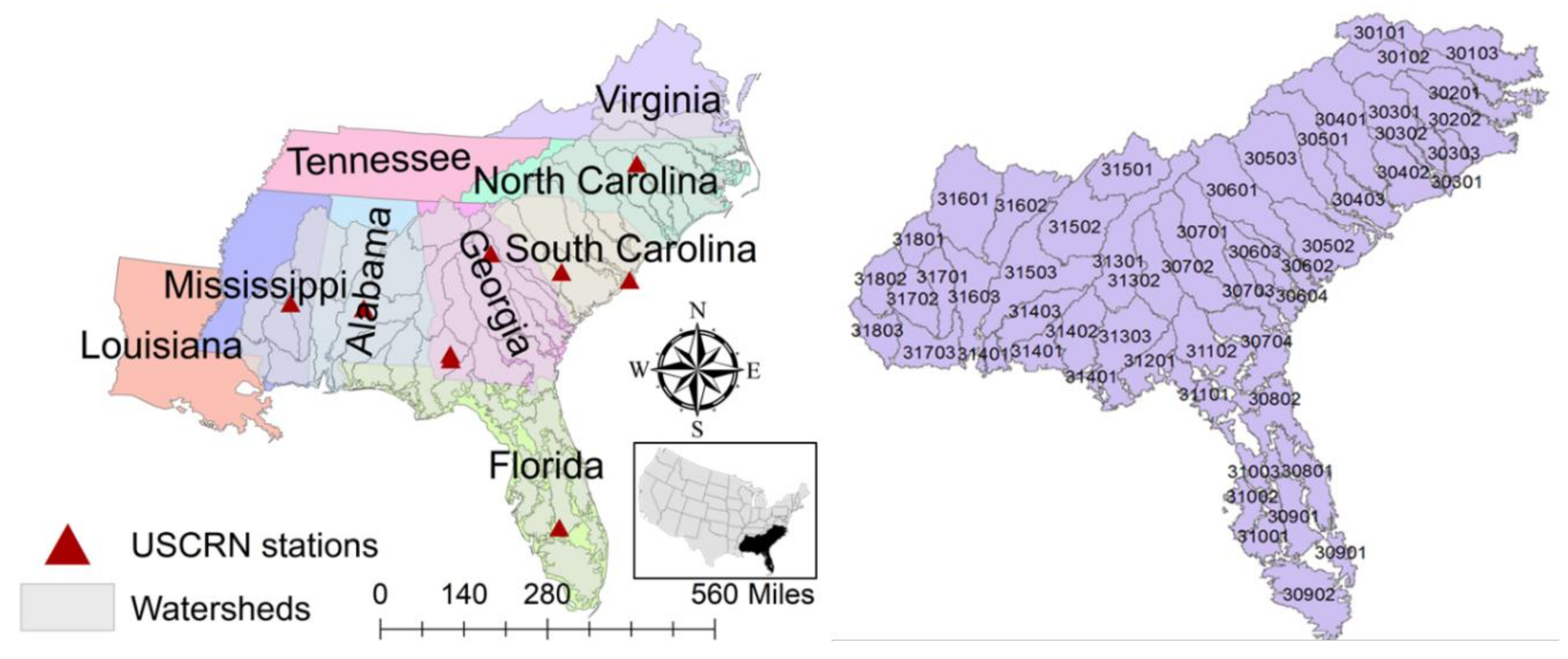
3.1. Study Area
3.2. Model Dataset
4. Methods
4.1. Modeling Framework
4.2. Calibration of SWAT Model Using the Sequential Uncertainty Fitting (SUFI)-2 Algorithm
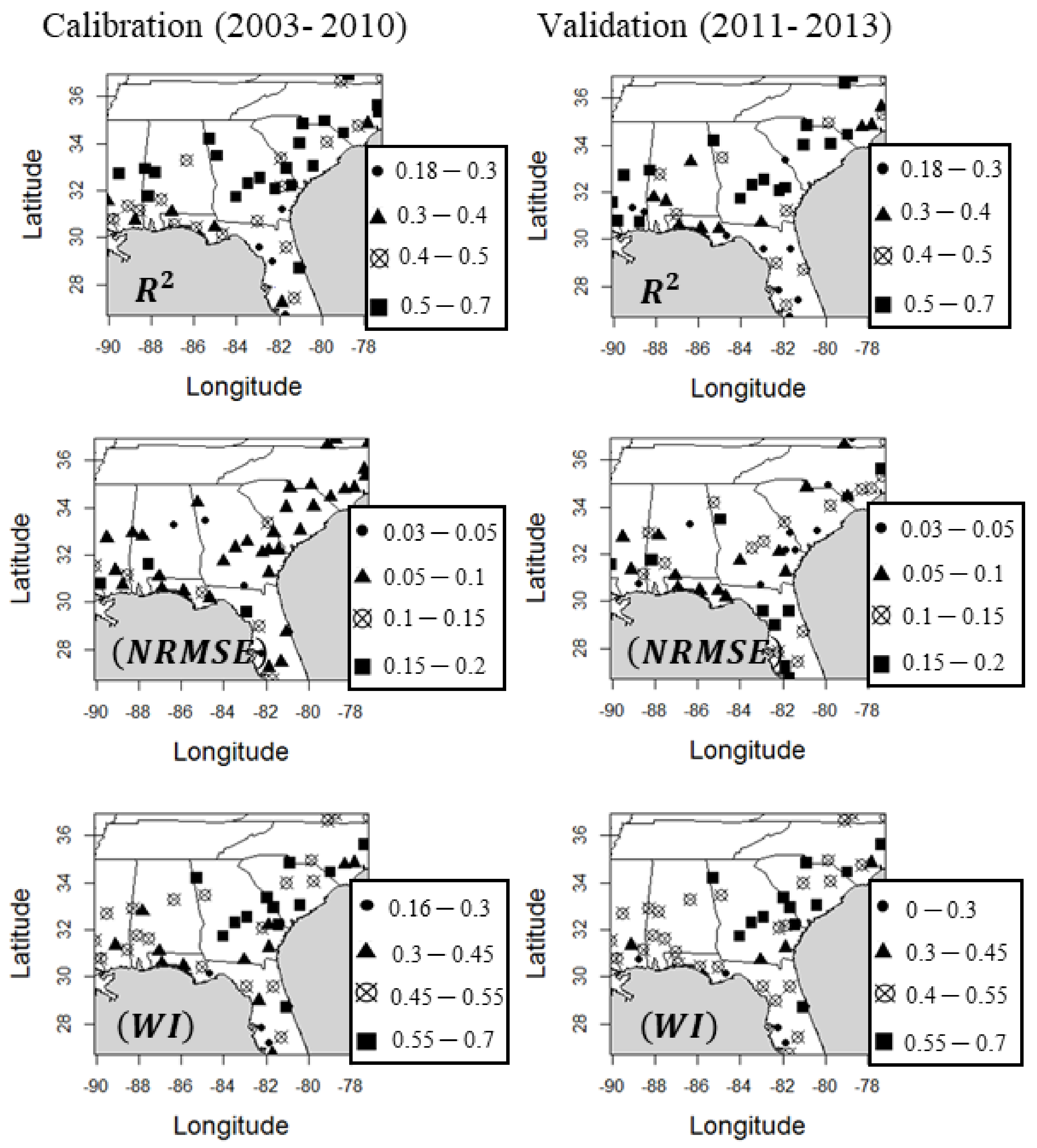
4.3. Performance Evaluation of the SWAT Model
4.4. Hydrologic Simulations Using the CFSv2-Integrated Calibrated SWAT Model
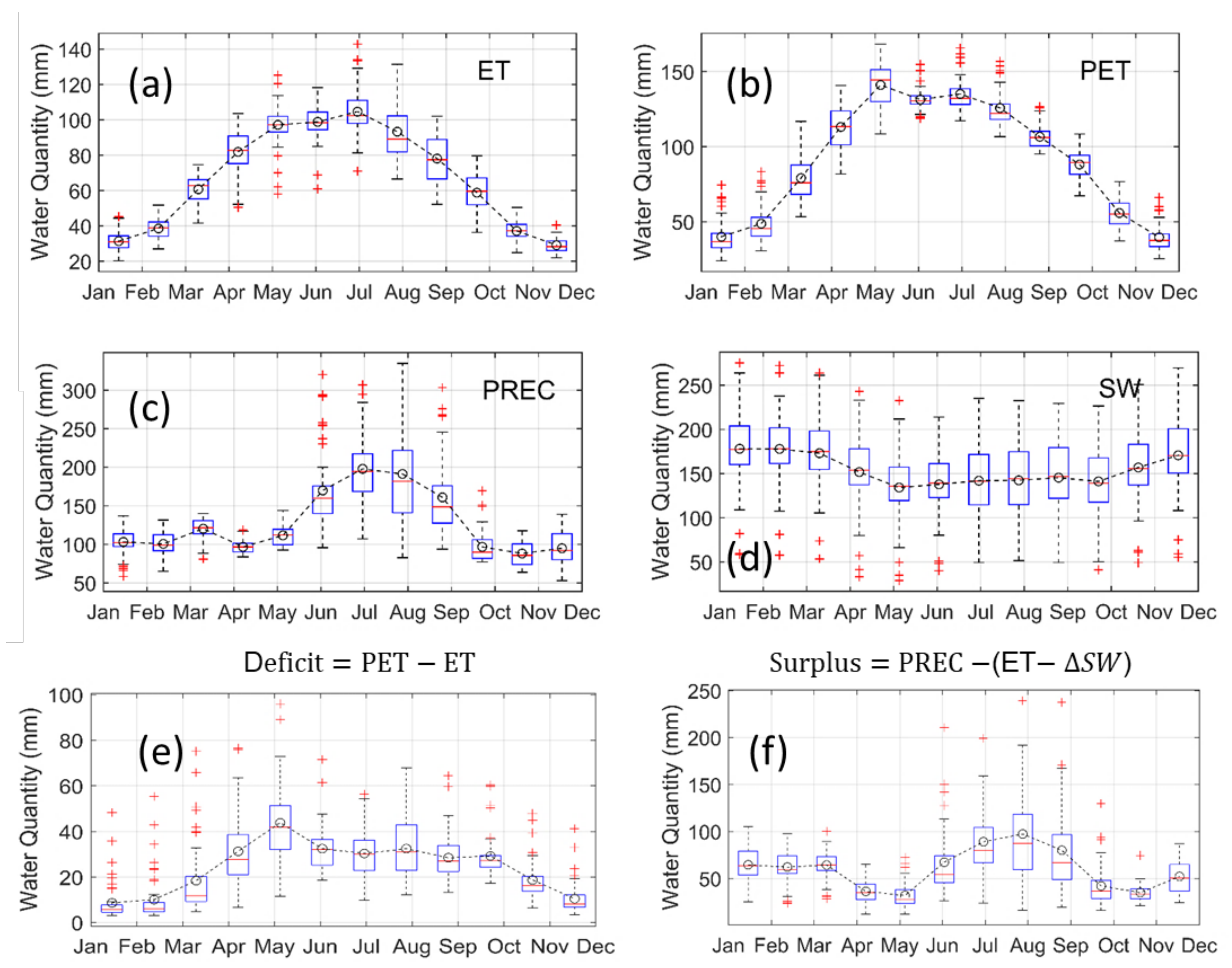
4.5. Water Balance Analysis
5. Results and Discussion
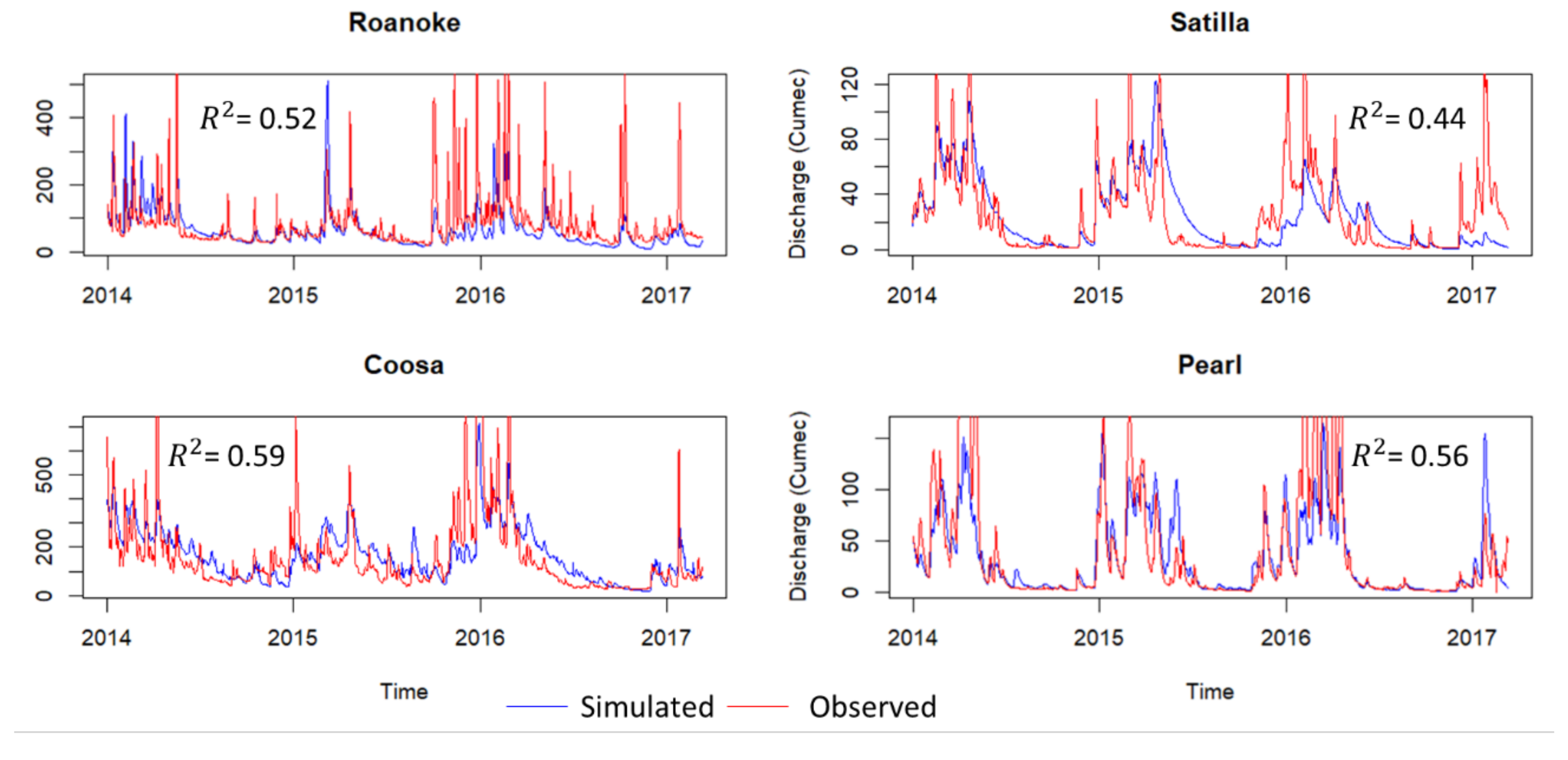
5.1. Streamflow Validation
5.2. Validation of Soil Moisture Data
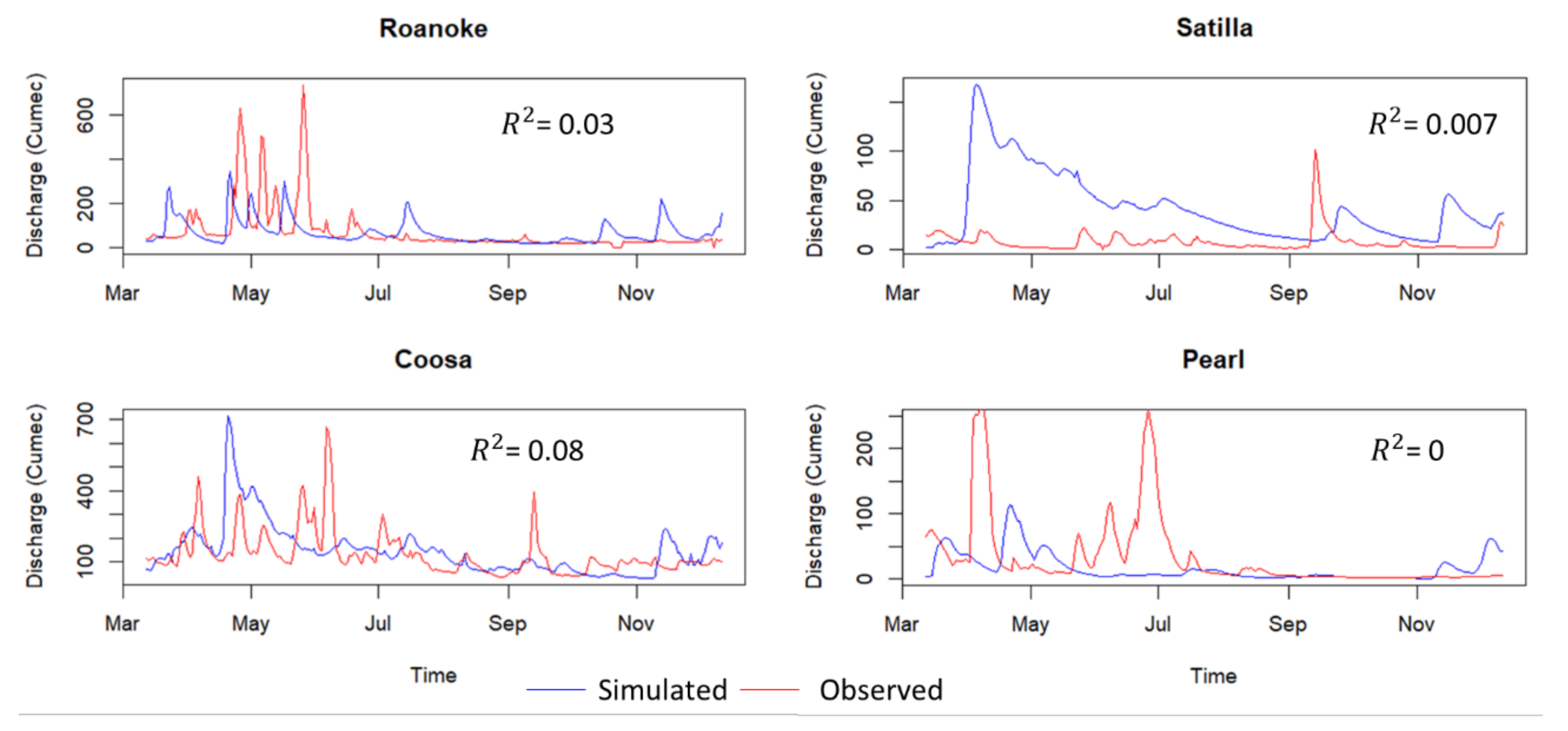
5.3. Near Real-Time Daily Simulations Using the CFSv2-Integrated SWAT Model
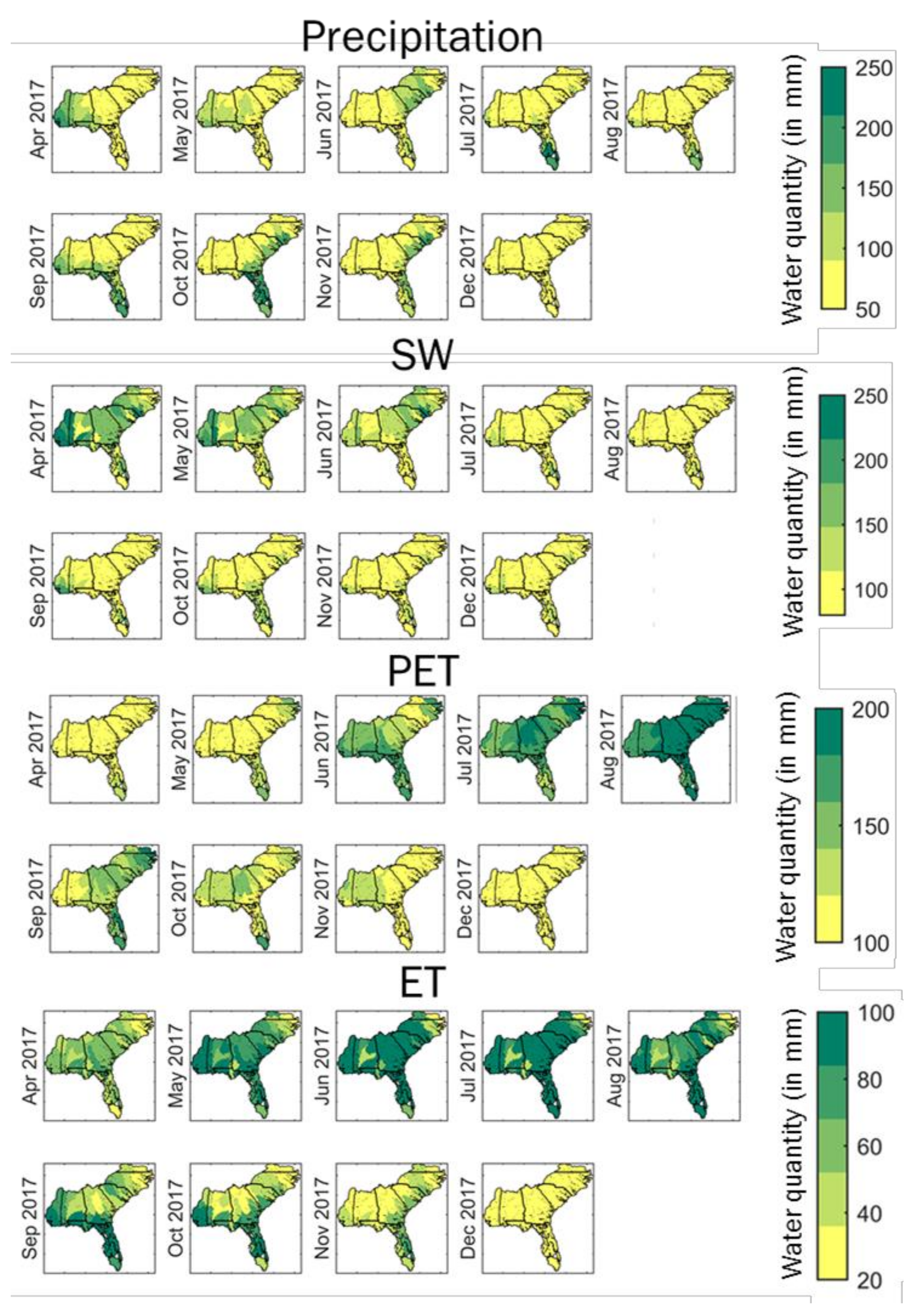
5.4. Water Budget Analysis for the SAG Region
5.5. Hydrological Forecasts for South Atlantic-Gulf Region Using the CFSv2-Integrated SWAT Model
5.6. Uncertainty in Model Outputs
6. Conclusions
Supplementary Materials
Author Contributions
Funding
Conflicts of Interest
Abbreviations
| SWAT | Soil and Water Assessment Tool |
| SM | Soil moisture |
| ET | Actual Evapotranspiration |
| PET | Potential Evapotranspiration |
| HUC-12 | A 12-digit Hydrologic Unit Code |
| USGS | U.S. Geological Survey |
| USCRN | U.S. Climate Reference Network |
| CFSv2 | National Centers for Environmental Prediction coupled forecast system model version 2 |
References
- Mu, Q.; Zhao, M.; Kimball, J.S.; McDowell, N.G.; Running, S.W. A remotely sensed global terrestrial drought severity index. Bull. Am. Meteorol. Soc. 2013, 94, 83–98. [Google Scholar] [CrossRef]
- Hanjra, M.A.; Qureshi, M.E. Global water crisis and future food security in an era of climate change. Food Policy 2010, 35, 365–377. [Google Scholar] [CrossRef]
- Sheffield, J.; Wood, E.F.; Chaney, N.; Guan, K.; Sadri, S.; Yuan, X.; Olang, L.; Amani, A.; Ali, A.; Demuth, S. A drought monitoring and forecasting system for sub-Sahara African water resources and food security. Bull. Am. Meteorol. Soc. 2014, 95, 861–882. [Google Scholar] [CrossRef]
- Pederson, N.; Bell, A.R.; Knight, T.A.; Leland, C.; Malcomb, N.; Anchukaitis, K.J.; Tackett, K.; Scheff, J.; Brice, A.; Catron, B. A long-term perspective on a modern drought in the American southeast. Environ. Res. Lett. 2012, 7, 014034. [Google Scholar] [CrossRef]
- Manuel, J. Drought in the southeast: Lessons for water management. Environ. Health Perspect. 2008, 116, 168–171. [Google Scholar] [CrossRef]
- Seager, R.; Tzanova, A.; Nakamura, J. Drought in the southeastern United States: Causes, variability over the last millennium, and the potential for future hydroclimate change. J. Clim. 2009, 22, 5021–5045. [Google Scholar] [CrossRef]
- Nagy, R.; Lockaby, B.G.; Helms, B.; Kalin, L.; Stoeckel, D. Water resources and land use and cover in a humid region: The southeastern United States. J. Environ. Qual. 2011, 40, 867–878. [Google Scholar] [CrossRef] [PubMed]
- U.S. Census Bureau. Interim State Population Projections; U.S. Census Bureau: Washington, DC, USA, 2005.
- Scasta, J.D.; Weir, J.R.; Stambaugh, M.C. Droughts and wildfires in western us rangelands. Rangelands 2016, 38, 197–203. [Google Scholar] [CrossRef]
- Madadgar, S.; Moradkhani, H. Spatio-temporal drought forecasting within Bayesian networks. J. Hydrol. 2014, 512, 134–146. [Google Scholar] [CrossRef]
- Lu, J.; Sun, G.; McNulty, S.G.; Amatya, D.M. Modeling actual evapotranspiration from forested watersheds across the southeastern united states. J. Am. Water Resour. Assoc. 2003, 39, 886–896. [Google Scholar] [CrossRef]
- Limaye, A.S.; Boyington, T.M.; Cruise, J.F.; Bulusu, A.; Brown, E. Macroscale hydrologic modeling for regional climate assessment studies in the southeastern united states. J. Am. Water Resour. Assoc. 2001, 37, 709–722. [Google Scholar] [CrossRef]
- Sun, S.; Chen, B.; Shao, Q.; Chen, J.; Liu, J.; Zhang, X.-j.Z.; Zhang, H.; Lin, X. Modeling evapotranspiration over China’s landmass from 1979 to 2012 using multiple land surface models: Evaluations and analyses. J. Hydrometeorol. 2017, 18, 1185–1203. [Google Scholar] [CrossRef]
- Ciabatta, L.; Brocca, L.; Massari, C.; Moramarco, T.; Gabellani, S.; Puca, S.; Wagner, W. Rainfall-runoff modelling by using sm2rain-derived and state-of-the-art satellite rainfall products over Italy. Int. J. Appl. Earth Obs. Geoinf. 2016, 48, 163–173. [Google Scholar] [CrossRef]
- Brocca, L.; Melone, F.; Moramarco, T.; Wagner, W.; Naeimi, V.; Bartalis, Z.; Hasenauer, S. Improving runoff prediction through the assimilation of the ascat soil moisture product. Hydrol. Earth Syst. Sci. 2010, 14, 1881–1893. [Google Scholar] [CrossRef]
- Laiolo, P.; Gabellani, S.; Campo, L.; Silvestro, F.; Delogu, F.; Rudari, R.; Pulvirenti, L.; Boni, G.; Fascetti, F.; Pierdicca, N. Impact of different satellite soil moisture products on the predictions of a continuous distributed hydrological model. Int. J. Appl. Earth Obs. Geoinf. 2016, 48, 131–145. [Google Scholar] [CrossRef]
- Bangira, T.; Maathuis, B.H.; Dube, T.; Gara, T.W. Investigating flash floods potential areas using ascat and trmm satellites in the western cape province, South Africa. Geocartol. Int. 2015, 30, 737–754. [Google Scholar] [CrossRef]
- Alvarez-Garreton, C.; Ryu, D.; Western, A.; Su, C.-H.; Crow, W.; Robertson, D.; Leahy, C. Improving operational flood ensemble prediction by the assimilation of satellite soil moisture: Comparison between lumped and semi-distributed schemes. Hydrol. Earth Syst. Sci. 2015, 19, 1659–1676. [Google Scholar] [CrossRef]
- Nanda, T.; Sahoo, B.; Beria, H.; Chatterjee, C. A wavelet-based non-linear autoregressive with exogenous inputs (wnarx) dynamic neural network model for real-time flood forecasting using satellite—Based rainfall products. J. Hydrol. 2016, 539, 57–73. [Google Scholar] [CrossRef]
- Hobbins, M.T.; Wood, A.; McEvoy, D.J.; Huntington, J.L.; Morton, C.; Anderson, M.; Hain, C. The evaporative demand drought index. Part i: Linking drought evolution to variations in evaporative demand. J. Hydrometeorol. 2016, 17, 1745–1761. [Google Scholar] [CrossRef]
- Anderson, M.C.; Norman, J.M.; Mecikalski, J.R.; Otkin, J.A.; Kustas, W.P. A climatological study of evapotranspiration and moisture stress across the continental United States based on thermal remote sensing: 1. Model formulation. J. Geophys. Res. Atmos. 2007, 112. [Google Scholar] [CrossRef]
- Sridhar, V.; Hubbard, K.G.; You, J.; Hunt, E.D. Development of the soil moisture index to quantify agricultural drought and its “user friendliness” in severity-area-duration assessment. J. Hydrometeorol. 2008, 9, 660–676. [Google Scholar] [CrossRef]
- Zhang, Y.; Peña-Arancibia, J.L.; McVicar, T.R.; Chiew, F.H.; Vaze, J.; Liu, C.; Lu, X.; Zheng, H.; Wang, Y.; Liu, Y.Y. Multi-decadal trends in global terrestrial evapotranspiration and its components. Sci. Rep. 2016, 6, 19124. [Google Scholar] [CrossRef] [PubMed]
- Mao, J.; Fu, W.; Shi, X.; Ricciuto, D.M.; Fisher, J.B.; Dickinson, R.E.; Wei, Y.; Shem, W.; Piao, S.; Wang, K. Disentangling climatic and anthropogenic controls on global terrestrial evapotranspiration trends. Environ. Res. Lett. 2015, 10, 094008. [Google Scholar] [CrossRef]
- Sehgal, V. Near Real-Time Seasonal Drought Forecasting and Retrospective Drought Analysis Using Simulated Multi-Layer Soil Moisture From Hydrological Models at Sub-Watershed Scales. Master’s Thesis, Virginia Tech, Blacksburg, VA, USA, 2017. [Google Scholar]
- Sehgal, V.; Sridhar, V.; Tyagi, A. Stratified drought analysis using a stochastic ensemble of simulated and in-situ soil moisture observations. J. Hydrol. 2017, 545, 226–250. [Google Scholar] [CrossRef]
- Sridhar, V.; Elliott, R.L.; Chen, F. Scaling effects on modeled surface energy-balance components using the noah-osu land surface model. J. Hydrol. 2003, 280, 105–123. [Google Scholar] [CrossRef]
- Sridhar, V.; Anderson, K. Human-induced modifications to boundary layer fluxes and their water management implications in a changing climate. Agric. For. Meteorol. 2017, 234, 66–79. [Google Scholar] [CrossRef]
- Garnaud, C.; Bélair, S.; Carrera, M.L.; McNairn, H.; Pacheco, A. Field-scale spatial variability of soil moisture and l-band brightness temperature from land surface modeling. J. Hydrometeorol. 2017, 18, 573–589. [Google Scholar] [CrossRef]
- Jimenez, C.; Prigent, C.; Aires, F. Toward an estimation of global land surface heat fluxes from multisatellite observations. J. Geophys. Res. Atmos. 2009, 114. [Google Scholar] [CrossRef]
- Jung, M.; Reichstein, M.; Bondeau, A. Towards global empirical upscaling of fluxnet eddy covariance observations: Validation of a model tree ensemble approach using a biosphere model. Biogeosciences 2009, 6, 2001–2013. [Google Scholar]
- Zhang, Y.; Leuning, R.; Hutley, L.B.; Beringer, J.; McHugh, I.; Walker, J.P. Using long-term water balances to parameterize surface conductances and calculate evaporation at 0.05 spatial resolution. Water Resour. Res. 2010, 46. [Google Scholar] [CrossRef]
- Mueller, B.; Seneviratne, S.; Jimenez, C.; Corti, T.; Hirschi, M.; Balsamo, G.; Ciais, P.; Dirmeyer, P.; Fisher, J.; Guo, Z. Evaluation of global observations-based evapotranspiration datasets and ipcc ar4 simulations. Geophys. Res. Lett. 2011, 38. [Google Scholar] [CrossRef]
- Vinukollu, R.K.; Wood, E.F.; Ferguson, C.R.; Fisher, J.B. Global estimates of evapotranspiration for climate studies using multi-sensor remote sensing data: Evaluation of three process-based approaches. Remote Sens. Environ. 2011, 115, 801–823. [Google Scholar] [CrossRef]
- Polhamus, A.; Fisher, J.B.; Tu, K.P. What controls the error structure in evapotranspiration models? Agric. For. Meteorol. 2013, 169, 12–24. [Google Scholar] [CrossRef]
- Muttiah, R.S.; Wurbs, R.A. Scale-dependent soil and climate variability effects on watershed water balance of the swat model. J. Hydrol. 2002, 256, 264–285. [Google Scholar] [CrossRef]
- Cao, W.; Bowden, W.B.; Davie, T.; Fenemor, A. Multi-variable and multi-site calibration and validation of swat in a large mountainous catchment with high spatial variability. Hydrol. Process. 2006, 20, 1057–1073. [Google Scholar] [CrossRef]
- Xu, Z.; Pang, J.; Liu, C.; Li, J. Assessment of runoff and sediment yield in the miyun reservoir catchment by using swat model. Hydrol. Process. 2009, 23, 3619–3630. [Google Scholar] [CrossRef]
- Yan, D.; Shi, X.; Yang, Z.; Li, Y.; Zhao, K.; Yuan, Y. Modified palmer drought severity index based on distributed hydrological simulation. Math. Probl. Eng. 2013, 2013, 327374. [Google Scholar] [CrossRef]
- Marek, G.W.; Gowda, P.H.; Evett, S.R.; Baumhardt, R.L.; Brauer, D.K.; Howell, T.A.; Marek, T.H.; Srinivasan, R. Estimating evapotranspiration for dryland cropping systems in the semiarid Texas high plains using swat. JAWRA J. Am. Water Resour. Assoc. 2016, 52, 298–314. [Google Scholar] [CrossRef]
- Wetterhall, F.; Winsemius, H.; Dutra, E.; Werner, M.; Pappenberger, E. Seasonal predictions of agro-meteorological drought indicators for the Limpopo basin. Hydrol. Earth Syst. Sci. 2015, 19, 2577–2586. [Google Scholar] [CrossRef]
- Shah, R.D.; Mishra, V. Utility of global ensemble forecast system (gefs) reforecast for medium-range drought prediction in India. J. Hydrometeorol. 2016, 17, 1781–1800. [Google Scholar] [CrossRef]
- Hansen, J.W. Integrating seasonal climate prediction and agricultural models for insights into agricultural practice. Philos. Trans. R. Soc. Lond. B Biol. Sci. 2005, 360, 2037–2047. [Google Scholar] [CrossRef] [PubMed]
- Shafiee-Jood, M.; Cai, X.; Chen, L.; Liang, X.Z.; Kumar, P. Assessing the value of seasonal climate forecast information through an end-to-end forecasting framework: Application to us 2012 drought in central Illinois. Water Resour. Res. 2014, 50, 6592–6609. [Google Scholar] [CrossRef]
- Dutra, E.; Magnusson, L.; Wetterhall, F.; Cloke, H.L.; Balsamo, G.; Boussetta, S.; Pappenberger, F. The 2010–2011 drought in the horn of Africa in ecmwf reanalysis and seasonal forecast products. Int. J. Climatol. 2013, 33, 1720–1729. [Google Scholar] [CrossRef]
- Ma, F.; Yuan, X.; Ye, A. Seasonal drought predictability and forecast skill over china. J. Geophys. Res. Atmos. 2015, 120, 8264–8275. [Google Scholar] [CrossRef]
- Crane, T.A.; Roncoli, C.; Paz, J.; Breuer, N.; Broad, K.; Ingram, K.T.; Hoogenboom, G. Forecast skill and farmers’ skills: Seasonal climate forecasts and agricultural risk management in the southeastern United States. Weather Clim. Soc. 2010, 2, 44–59. [Google Scholar] [CrossRef]
- Gunda, T.; Bazuin, J.; Nay, J.; Yeung, K. Impact of seasonal forecast use on agricultural income in a system with varying crop costs and returns: An empirically-grounded simulation. Environ. Res. Lett. 2017, 12, 034001. [Google Scholar] [CrossRef]
- Mo, K.C.; Long, L.N.; Xia, Y.; Yang, S.; Schemm, J.E.; Ek, M. Drought indices based on the climate forecast system reanalysis and ensemble nldas. J. Hydrometeorol. 2011, 12, 181–205. [Google Scholar] [CrossRef]
- Dirmeyer, P.A. Characteristics of the water cycle and land–atmosphere interactions from a comprehensive reforecast and reanalysis data set: Cfsv2. Clim. Dyn. 2013, 41, 1083–1097. [Google Scholar] [CrossRef]
- McEvoy, D.J.; Huntington, J.L.; Mejia, J.F.; Hobbins, M.T. Improved seasonal drought forecasts using reference evapotranspiration anomalies. Geophys. Res. Lett. 2016, 43, 377–385. [Google Scholar] [CrossRef]
- Mo, K.C.; Shukla, S.; Lettenmaier, D.P.; Chen, L.C. Do climate forecast system (cfsv2) forecasts improve seasonal soil moisture prediction? Geophys. Res. Lett. 2012, 39. [Google Scholar] [CrossRef]
- Roundy, J.K.; Ferguson, C.R.; Wood, E.F. Impact of land-atmospheric coupling in cfsv2 on drought prediction. Clim. Dyn. 2014, 43, 421–434. [Google Scholar] [CrossRef]
- Mace, R.E.; Yang, B.; Pu, B. Early Warning of Summer Drought over Texas and the South Central United States: Spring Conditions as a Harbinger of Summer Drought; Technical note; Texas Water Development Board, Austin: Austin, TX, USA, 2015. [Google Scholar]
- Zhang, X.; Tang, Q.; Liu, X.; Leng, G.; Li, Z. Soil moisture drought monitoring and forecasting using satellite and climate model data over southwestern China. J. Hydrometeorol. 2017, 18, 5–23. [Google Scholar] [CrossRef]
- Saha, S.; Moorthi, S.; Pan, H.-L.; Wu, X.; Wang, J.; Nadiga, S.; Tripp, P.; Kistler, R.; Woollen, J.; Behringer, D. The ncep climate forecast system reanalysis. Bull. Am. Meteorol. Soc. 2010, 91, 1015–1058. [Google Scholar] [CrossRef]
- Kang, H.; Sridhar, V. Improved drought prediction using near real-time climate forecasts and simulated hydrologic conditions. Sustainability 2018, 10, 1799. [Google Scholar] [CrossRef]
- Kang, H.; Sridhar, V. Combined statistical and spatially distributed hydrological model for evaluating future drought indices in Virginia. J. Hydrol. Reg. Stud. 2017, 12, 253–272. [Google Scholar] [CrossRef]
- Sehgal, V.; Sridhar, V. Effect of hydroclimatological teleconnections on the watershed-scale drought predictability in the southeastern US. Int. J. Climatol. 2018, 38, e1139–e1157. [Google Scholar] [CrossRef]
- Suliman, A.H.A.; Jajarmizadeh, M.; Harun, S.; Darus, I.Z.M. Comparison of semi-distributed, gis-based hydrological models for the prediction of streamflow in a large catchment. Water Resour. Manag. 2015, 29, 3095–3110. [Google Scholar] [CrossRef]
- Neitsch, S.L.; Arnold, J.G.; Kiniry, J.R.; Williams, J.R. Soil and Water Assessment Tool Theoretical Documentation Version 2009; Texas Water Resources Institute, Texas A&M University: College Station, TX, USA, 2011. [Google Scholar]
- Arnold, J.G.; Moriasi, D.N.; Gassman, P.W.; Abbaspour, K.C.; White, M.J.; Srinivasan, R.; Santhi, C.; Harmel, R.; Van Griensven, A.; Van Liew, M.W. Swat: Model use, calibration, and validation. Trans. ASABE 2012, 55, 1491–1508. [Google Scholar] [CrossRef]
- Gassman, P.; Reyes, M.; Green, C.; Arnold, J. The soil and water assessment tool: Historical development, applications, and future research directions. Trans. Am. Soc. Agric. Biol. Eng. 2007, 50, 1211–1250. [Google Scholar] [CrossRef]
- Arnold, J.G.; Srinivasan, R.; Muttiah, R.S.; Williams, J.R. Large area hydrologic modeling and assessment part i: model development1. J. Am. Water Resour. Assoc. 1998, 34, 73–89. [Google Scholar] [CrossRef]
- Liu, Y.; Yang, W.; Wang, X. Development of a swat extension module to simulate riparian wetland hydrologic processes at a watershed scale. Hydrol. Process. 2008, 22, 2901–2915. [Google Scholar] [CrossRef]
- Williams, J.; Jones, C.; Dyke, P. A modeling approach to determining the relationship between erosion and soil productivity. Trans. ASAE 1984, 27, 129–144. [Google Scholar] [CrossRef]
- SWAT. Swat Literature Database for Peer-Reviewed Journal Articles; Center for Agricultural and Rural Development: Ames, IA, USA, 2017. [Google Scholar]
- United States Geological Survey. Boundary Descriptions and Names of Regions, Subregions, Accounting Units and Cataloging Units; USGS: Reston, NA, USA, 2017. [Google Scholar]
- McEvoy, D.J. Physically Based Evaporative Demand as a Drought Metric: Historical Analysis and Seasonal Prediction. Ph.D. Thesis, University of Nevada, Reno, NV, USA, 2015. [Google Scholar]
- Homer, C.G.; Dewitz, J.A.; Yang, L.; Jin, S.; Danielson, P.; Xian, G.; Coulston, J.; Herold, N.D.; Wickham, J.; Megown, K. Completion of the 2011 national land cover database for the conterminous united states-representing a decade of land cover change information. Photogramm. Eng. Remote Sens. 2015, 81, 345–354. [Google Scholar]
- Dile, Y.T.; Srinivasan, R. Evaluation of cfsr climate data for hydrologic prediction in data-scarce watersheds: An application in the blue nile river basin. JAWRA J. Am. Water Resour. Assoc. 2014, 50, 1226–1241. [Google Scholar] [CrossRef]
- Tuo, Y.; Duan, Z.; Disse, M.; Chiogna, G. Evaluation of precipitation input for SWAT modeling in Alpine catchment: A case study in the Adige river basin (Italy). Sci. Total Environ. 2016, 573, 66–82. [Google Scholar] [CrossRef] [PubMed]
- Vu, M.; Raghavan, S.V.; Liong, S.Y. Swat use of gridded observations for simulating runoff-a Vietnam river basin study. Hydrol. Earth Syst. Sci. 2012, 16, 2801–2811. [Google Scholar] [CrossRef]
- Duethmann, D.; Zimmer, J.; Gafurov, A.; Güntner, A.; Kriegel, D.; Merz, B.; Vorogushyn, S. Evaluation of areal precipitation estimates based on downscaled reanalysis and station data by hydrological modelling. Hydrol. Earth Syst. Sci. 2013, 17, 2415–2434. [Google Scholar] [CrossRef]
- Yang, Y.; Wang, G.; Wang, L.; Yu, J.; Xu, Z. Evaluation of gridded precipitation data for driving swat model in area upstream of three gorges reservoir. PLoS ONE 2014, 9, e112725. [Google Scholar] [CrossRef] [PubMed]
- Abbaspour, K.C.; van Genuchten, M.T.; Schulin, R.; Schläppi, E. A sequential uncertainty domain inverse procedure for estimating subsurface flow and transport parameters. Water Resour. Res. 1997, 33, 1879–1892. [Google Scholar] [CrossRef]
- Abbaspour, K.; Johnson, C.; Van Genuchten, M.T. Estimating uncertain flow and transport parameters using a sequential uncertainty fitting procedure. Vadose Zone J. 2004, 3, 1340–1352. [Google Scholar] [CrossRef]
- Abbaspour, K.; Rouholahnejad, E.; Vaghefi, S.; Srinivasan, R.; Yang, H.; Kløve, B. A continental-scale hydrology and water quality model for Europe: Calibration and uncertainty of a high-resolution large-scale swat model. J. Hydrol. 2015, 524, 733–752. [Google Scholar] [CrossRef]
- Jin, X.; Sridhar, V. Impacts of climate change on hydrology and water resources in the Boise and Spokane river basins1. JAWRA J. Am. Water Resour. Assoc. 2012, 48, 197–220. [Google Scholar] [CrossRef]
- Rouholahnejad, E.; Abbaspour, K.C.; Vejdani, M.; Srinivasan, R.; Schulin, R.; Lehmann, A. A parallelization framework for calibration of hydrological models. Environ. Model. Softw. 2012, 31, 28–36. [Google Scholar] [CrossRef]
- Nash, J.E.; Sutcliffe, J.V. River flow forecasting through conceptual models part i—A discussion of principles. J. Hydrol. 1970, 10, 282–290. [Google Scholar] [CrossRef]
- Feyereisen, G.; Strickland, T.; Bosch, D.; Sullivan, D. Evaluation of swat manual calibration and input parameter sensitivity in the little river watershed. Trans. ASABE 2007, 50, 843–855. [Google Scholar] [CrossRef]
- Kang, H.; Sridhar, V. A statistical and distributed hydrological modeling combination to evaluate drought indices in Virginia. JAWRA J. Am. Water Resour. Assoc. 2017. [Google Scholar] [CrossRef]
- Wang, X.; Yang, W.; Melesse, A.M. Using hydrologic equivalent wetland concept within swat to estimate streamflow in watersheds with numerous Wetlands. Trans. ASAE 2008, 51, 55–72. [Google Scholar] [CrossRef]
- Van Liew, M.W.; Arnold, J.; Bosch, D. Problems and potential of autocalibrating a hydrologic model. Trans. ASAE 2005, 48, 1025–1040. [Google Scholar] [CrossRef]
- Uniyal, B.; Jha, M.K.; Verma, A.K. Parameter identification and uncertainty analysis for simulating streamflow in a river basin of eastern India. Hydrol. Process. 2015, 29, 3744–3766. [Google Scholar] [CrossRef]
- Kang, H.; Moon, J.; Shin, Y.; Ryu, J.; Kum, D.H.; Jang, C.; Choi, J.; Kong, D.S.; Lim, K.J. Modification of swat auto-calibration for accurate flow estimation at all flow regimes. Paddy Water Environ. 2016, 14, 499–508. [Google Scholar] [CrossRef]
- Martinez-Martinez, E.; Nejadhashemi, A.P.; Woznicki, S.A.; Love, B.J. Modeling the hydrological significance of wetland restoration scenarios. J. Environ. Manag. 2014, 133, 121–134. [Google Scholar] [CrossRef] [PubMed]
- Hovenga, P.A.; Wang, D.; Medeiros, S.C.; Hagen, S.C.; Alizad, K. The response of runoff and sediment loading in the Apalachicola river, Florida to climate and land use land cover change. Earth’s Future 2016, 4, 124–142. [Google Scholar] [CrossRef]
- Willmott, C.J.; Robeson, S.M.; Matsuura, K. A refined index of model performance. Int. J. Climatol. 2012, 32, 2088–2094. [Google Scholar] [CrossRef]
- Willmott, C.J.; Robeson, S.M.; Matsuura, K.; Ficklin, D.L. Assessment of three dimensionless measures of model performance. Environ. Model. Softw. 2015, 73, 167–174. [Google Scholar] [CrossRef]
- Koch, J.; Demirel, M.C.; Stisen, S. The spatial efficiency metric (spaef): Multiple-component evaluation of spatial patterns for optimization of hydrological models. Geosci. Model Dev. 2018, 11, 1873–1886. [Google Scholar] [CrossRef]
- Demirel, M.C.; Mai, J.; Mendiguren, G.; Koch, J.; Samaniego, L.; Stisen, S. Combining satellite data and appropriate objective functions for improved spatial pattern performance of a distributed hydrologic model. Hydrol. Earth Syst. Sci. 2018, 22, 1299–1315. [Google Scholar] [CrossRef]
- Tauro, F.; Selker, J.; van de Giesen, N.; Abrate, T.; Uijlenhoet, R.; Porfiri, M.; Manfreda, S.; Caylor, K.; Moramarco, T.; Benveniste, J. Measurements and observations in the xxi century (moxxi): Innovation and multi-disciplinarity to sense the hydrological cycle. Hydrol. Sci. J. 2018, 63, 169–196. [Google Scholar] [CrossRef]
- Sridhar, V.; Hubbard, K. Estimation of the water balance using observed soil water in the Nebraska sandhills. J. Hydrol. Eng. 2009, 15, 70–78. [Google Scholar] [CrossRef]
- Singh, R.; Prasad, V.H.; Bhatt, C. Remote sensing and gis approach for assessment of the water balance of a watershed/evaluation par télédétection et sig du bilan hydrologique d’un bassin versant. Hydrol. Sci. J. 2004, 49, 131–141. [Google Scholar] [CrossRef]
- Cho, J.; Bosch, D.; Vellidis, G.; Lowrance, R.; Strickland, T. Multi-site evaluation of hydrology component of swat in the coastal plain of southwest Georgia. Hydrol. Process. 2013, 27, 1691–1700. [Google Scholar] [CrossRef]
- Amatya, D.; Jha, M.K. Evaluating the swat model for a low-gradient forested watershed in coastal South Carolina. Trans. ASABE 2011, 54, 2151–2163. [Google Scholar] [CrossRef]
- Yang, J.; Reichert, P.; Abbaspour, K.; Xia, J.; Yang, H. Comparing uncertainty analysis techniques for a swat application to the chaohe basin in china. J. Hydrol. 2008, 358, 1–23. [Google Scholar] [CrossRef]
- Wu, H. Integrated Sensitivity Analysis, Calibration, and Uncertainty Propagation Analysis Approaches for Supporting Hydrological Modeling. Ph.D. Thesis, Memorial University of Newfoundland, St. John’s, NL, Canada, 2016. [Google Scholar]
- Beven, K.; Freer, J. Equifinality, data assimilation, and uncertainty estimation in mechanistic modelling of complex environmental systems using the glue methodology. J. Hydrol. 2001, 249, 11–29. [Google Scholar] [CrossRef]
- Moreda, F.; Koren, V.; Zhang, Z.; Reed, S.; Smith, M. Parameterization of distributed hydrological models: Learning from the experiences of lumped modeling. J. Hydrol. 2006, 320, 218–237. [Google Scholar] [CrossRef]
- Fu, C.; James, A.L.; Yao, H. Investigations of uncertainty in swat hydrologic simulations: A case study of a Canadian Shield catchment. Hydrol. Process. 2015, 29, 4000–4017. [Google Scholar] [CrossRef]
- Abbaspour, K.C. Swat-Cup4: Swat Calibration and Uncertainty Programs—A User Manual; Swiss Federal Institute of Aquatic Science and Technology, Eawag: Zurich, Switzerland, 2011. [Google Scholar]
- Lang, Y.; Ye, A.; Gong, W.; Miao, C.; Di, Z.; Xu, J.; Liu, Y.; Luo, L.; Duan, Q. Evaluating skill of seasonal precipitation and temperature predictions of ncep cfsv2 forecasts over 17 hydroclimatic regions in china. J. Hydrometeorol. 2014, 15, 1546–1559. [Google Scholar] [CrossRef]
- Yuan, X.; Wood, E.F.; Luo, L.; Pan, M. A first look at climate forecast system version 2 (cfsv2) for hydrological seasonal prediction. Geophys. Res. Lett. 2011, 38. [Google Scholar] [CrossRef]
- Kim, H.-M.; Webster, P.J.; Curry, J.A. Seasonal prediction skill of ecmwf system 4 and ncep cfsv2 retrospective forecast for the northern hemisphere winter. Clim. Dyn. 2012, 39, 2957–2973. [Google Scholar] [CrossRef]
- Sridhar, V.; Jaksa, W.T.; Huntington, J.L. Spatial mapping of evapotranspiration using the complementary relationship in the natural ecosystems. In Evapotranspiration; Er-Raki, S., Ed.; Nova Science Publishers, Inc.: New York, NY, USA, 2013. [Google Scholar]
- Jaksa, W.T.; Sridhar, V.; Huntington, J.L.; Khanal, M. Evaluation of the complementary relationship using noah land surface model and north American regional reanalysis (narr) data to estimate evapotranspiration in semiarid ecosystems. J. Hydrometeorol. 2013, 14, 345–359. [Google Scholar] [CrossRef]


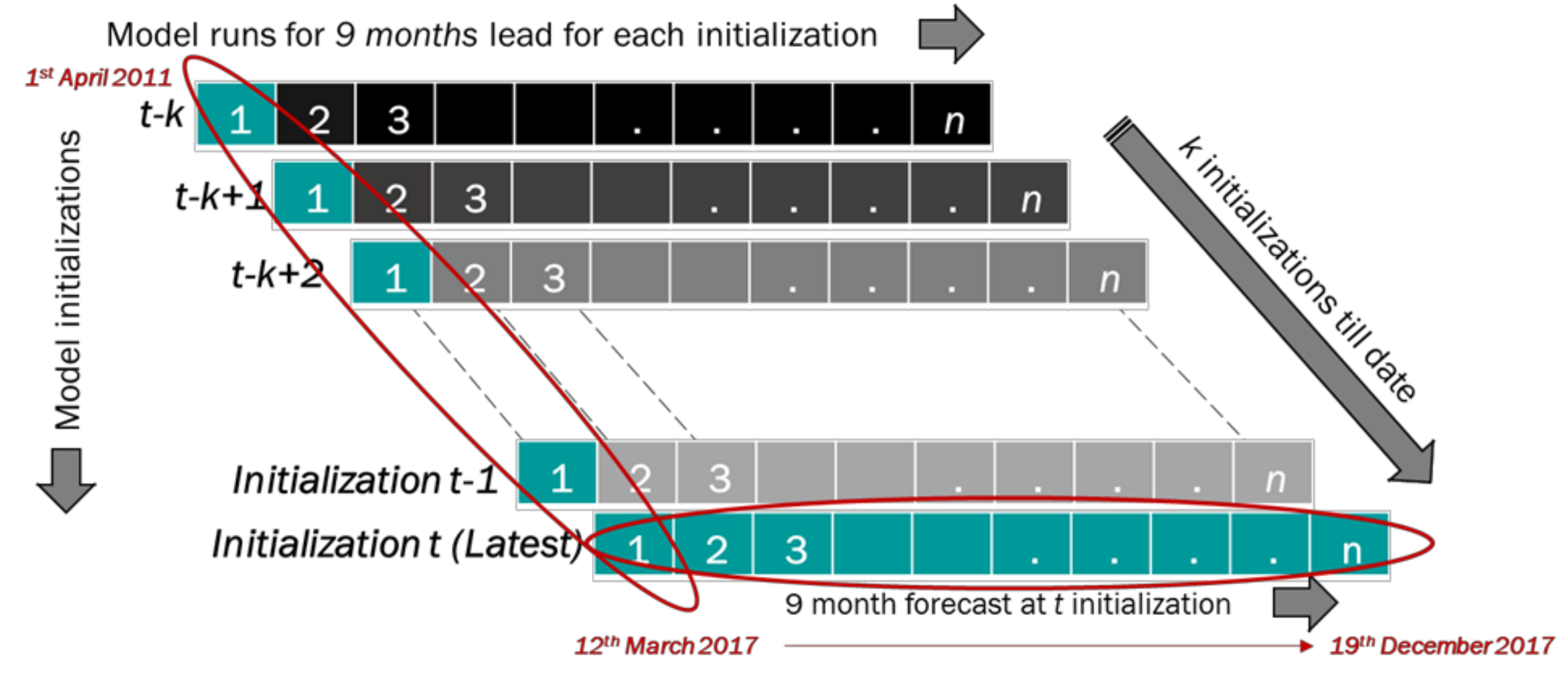
| Initialization Month | Total Members | Initialization Days |
|---|---|---|
| January | 28 | 1, 6, 11, 16, 21, 26, 31 |
| February | 20 | 5, 10, 15, 20, 25 |
| March | 24 | 2, 7, 12, 17, 22, 27 |
| April | 24 | 1, 6, 11, 16, 21, 26 |
| May | 28 | 1, 6, 11, 16, 21, 26, 31 |
| June | 24 | 5, 10, 15, 20, 25, 30 |
| July | 24 | 5, 10, 15, 20, 25, 30 |
| August | 24 | 4, 9, 14, 19, 24, 29 |
| September | 24 | 3, 8, 13, 18, 23, 28 |
| October | 24 | 3, 8, 13, 18, 23, 28 |
| November | 24 | 2, 7, 12, 17, 22, 27 |
| December | 24 | 2, 7, 12, 17, 22, 27 |
| Basin | USGS Station | Watershed | River/Basin | Basin | USGS Station | Watershed | River/Basin |
|---|---|---|---|---|---|---|---|
| 0301 | 02066000 | 030101 | Roanoke | 0309 | 02292900 | 030902 | Caloosahatchee |
| 02075500 | 030102 | Dan | 0310 | 02296750 | 031001 | Peace | |
| 02047000 | 030103 | Nottoway | 02301500 | 031002 | Alafia | ||
| 0302 | 02084000 | 030201 | Tar | 02313000 | 031003 | Withlacoochee | |
| 02091814 | 030202 | Neuse | 0311 | 02323500 | 031101 | Suwannee | |
| 0303 | 02134500 | 030301 | Lumber | 02317500 | 031102 | Alapaha | |
| 02106500 | 030302 | Black | 0312 | 02330150 | 031201 | Ochlockonee | |
| 02108000 | 030303 | NE Cape fear | 0313 | 02338000 | 031301 | Chattahoochee | |
| 0304 | 02129000 | 030401 | Pee Dee | 02350512 | 031302 | Flint | |
| 02134500 | 030402 | Lumber | 02358700 | 031303 | Apalachicola | ||
| 02132000 | 030403 | Lynches | 0314 | 02369600 | 031401 | Yellow | |
| 0305 | 02147020 | 030501 | Catawba | 02366500 | 031402 | Choctawhatchee | |
| 02169500 | 030502 | Congaree | 02374250 | 031403 | Conecuh | ||
| 02175000 | 030503 | Edisto | 0315 | 02397000 | 031501 | Coosa (Rome) | |
| 0306 | 02197000 | 030601 | Savannah | 02407000 | 031502 | Coosa (Childersburg) | |
| 02198000 | 030602 | Barrier Creek | 02428400 | 031503 | Alabama | ||
| 02202500 | 030603 | Ogeechee | 0316 | 02448500 | 031601 | Noxubee | |
| 02203000 | 030604 | Canoochee | 02466030 | 031602 | Black warrior | ||
| 0307 | 02223500 | 030701 | Oconee | 02469761 | 031603 | Tombigbee | |
| 02215000 | 030702 | Ocmulgee | 0317 | 02478500 | 031701 | Chickasawhay | |
| 02225500 | 030703 | Ohoopee | 02474500 | 031702 | Tallahala | ||
| 02228000 | 030704 | Satilla | 02479300 | 031703 | Red Cr. | ||
| 0308 | 02234000 | 030801 | St. Johns (Geneva) | 0318 | 02482550 | 031801 | Pearl (Carthage) |
| 02244040 | 030802 | St. Johns (Buffalo bluff) | 02488500 | 031802 | Pearl (Monticello) | ||
| 0309 | 02270500 | 030901 | Arbuckle Cr. | 02489500 | 031803 | Pearl (Bogalusa) |
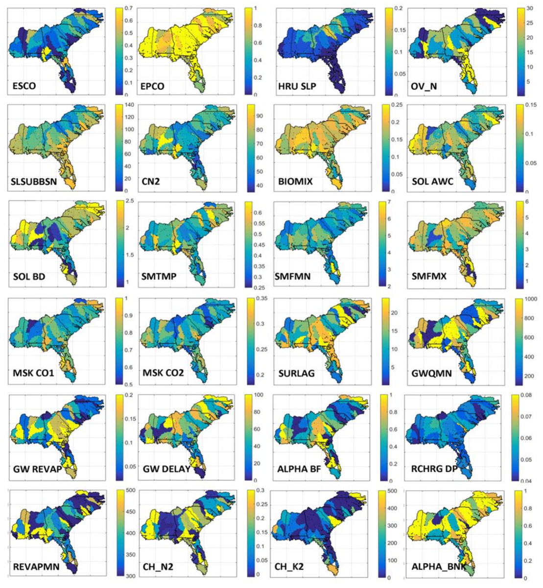
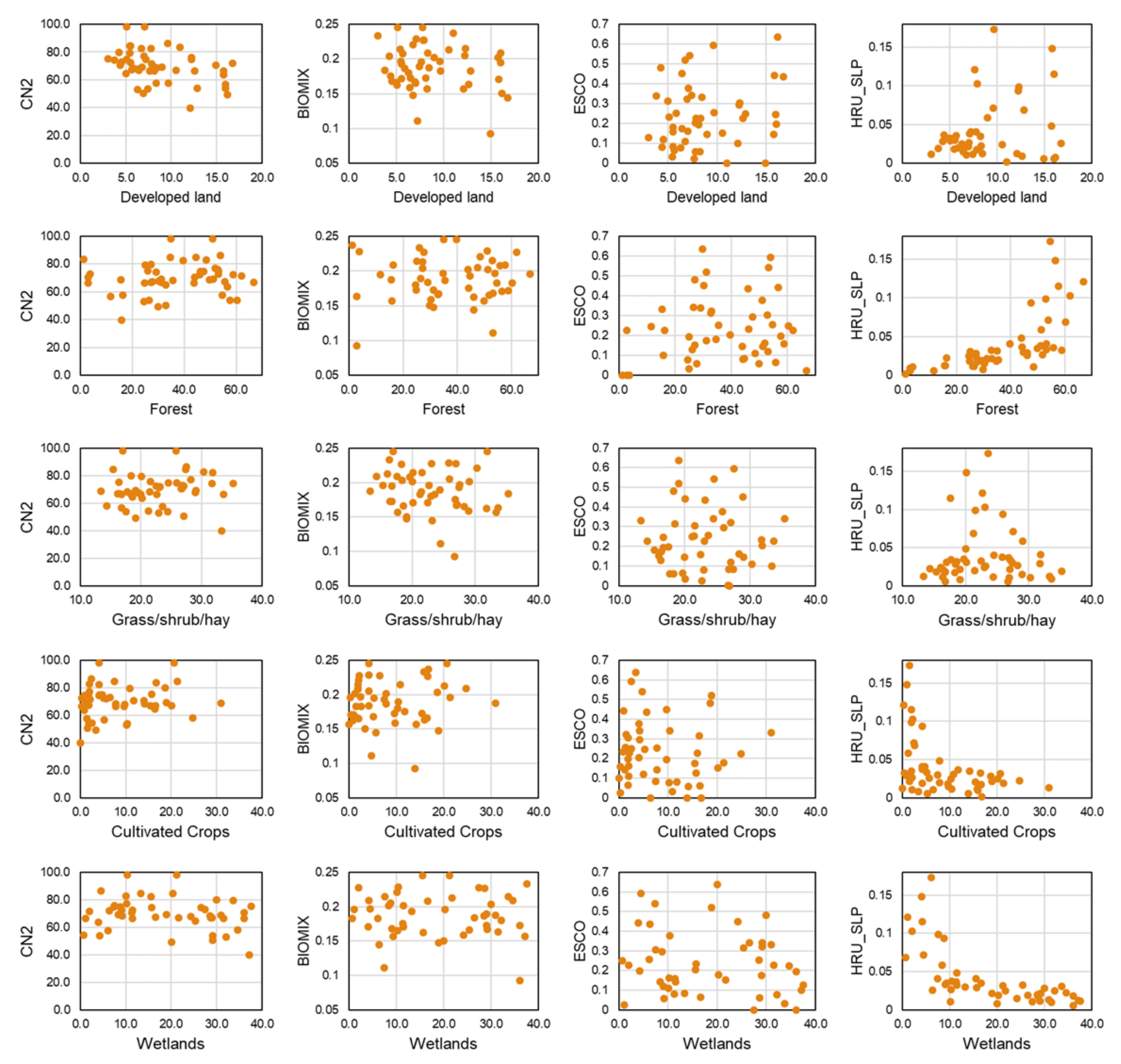
| Class | Name | Description | Method Used | Min. | Max. |
|---|---|---|---|---|---|
| HRU | ESCO | Soil evaporation compensation factor (unitless) | Replace (v) | 0 | 1 |
| EPCO | Plant evaporation compensation factor (unitless) | Relative (r) | −0.2 | 0.2 | |
| HRU_SLP | Average slope steepness (mm/mm) | Relative (r) | −0.2 | 0.2 | |
| OV_N | Manning’s “n” value for overland flow | Replace (v) | 0.01 | 30 | |
| SLSUBBSN | Average slope length (m) | Relative (r) | −0.2 | 0.2 | |
| MGT | CN2 | Initial SCS curve number for moisture condition II (unitless) | Relative (r) | −0.2 | 0.2 |
| BIOMIX | Biological mixing efficiency (unitless) | Relative (r) | −0.2 | 0.2 | |
| SOL | SOL_AWC | Available water capacity of the soil layer (mm⁄mm) | Relative (r) | −0.2 | 0.2 |
| SOL_BD | Moist bulk density (mg/m3 or g/cm3) | Replace (v) | 0.9 | 2.5 | |
| BSN | SMTMP | Snowmelt base temperature (°C) | Relative (r) | −0.2 | 0.2 |
| SMFMN | Melt factor for snow on Dec 21 (mm H2O/°C·day) | Relative (r) | −0.2 | 0.2 | |
| SMFMX | Melt factor for snow on June 21 (mm H2O/°C·day) | Relative (r) | −0.2 | 0.2 | |
| MSK_CO1 | Calibration coefficient used to control the impact of storage time constant (Km) for normal flow when Km is calculated for the reach | Relative (r) | −0.2 | 0.2 | |
| MSK_CO2 | Same as above, but for low flows | Relative (r) | −0.2 | 0.2 | |
| SURLAG | Surface runoff lag coefficient | Replace (v) | 0.05 | 24 | |
| GW | GWQMN | Threshold depth of water in the shallow aquifer required for return flow to occur (mm) | Replace (v) | 0 | 5000 |
| GW_REVAP | Groundwater revaporation coefficient (unitless) | Replace (v) | 0.02 | 0.2 | |
| GW_DELAY | Groundwater delay (days) | Replace (v) | 0 | 500 | |
| ALPHA_BF | Base flow alpha factor (days) | Replace (v) | 0 | 1 | |
| RCHRG_DP | Groundwater recharge to deep aquifer (fraction) | Relative (r) | −0.2 | 0.2 | |
| REVAPMN | Threshold depth of water in the shallow aquifer for revaporation to occur (mm) | Relative (r) | −0.2 | 0.2 | |
| RTE | CH_N2 | Manning coefficient for channel (unitless) | Replace (v) | −0.01 | 0.3 |
| CH_K2 | Effective channel hydraulic conductivity (mm⁄h) | Replace (v) | −0.01 | 500 | |
| ALPHA_BNK | Baseflow alpha factor for storage (days) | Replace (v) | 0 | 1 |
| Correlation | RMSE (m3/m3) | |||||
|---|---|---|---|---|---|---|
| Station location (Lat, Lon) | 10 cm | 20 cm | 50 cm | 10 cm | 20 cm | 50 cm |
| Durham, NC (35.97, −79.09) | 0.658 | 0.681 | 0.749 | 0.227 | 0.224 | 0.372 |
| Blackville, SC (33.36, −81.33) | 0.324 | 0.345 | 0.279 | 0.131 | 0.125 | 0.020 |
| McClellanville, SC (33.15, −79.36) | 0.550 | 0.543 | 0.502 | 0.080 | 0.017 | 0.076 |
| Watkinsville, GA (33.78, −83.39) | 0.581 | 0.602 | 0.643 | 0.043 | 0.012 | 0.078 |
| Sebring, FL (27.15, −81.37) | 0.424 | 0.436 | 0.533 | 0.081 | 0.029 | 0.100 |
| Newton (W), GA (31.31, −84.47) | 0.552 | 0.564 | 0.481 | 0.029 | 0.017 | 0.033 |
| Newton (SW), GA (31.19, −84.45) | 0.579 | 0.594 | 0.628 | 0.051 | 0.007 | 0.098 |
| Selma, AL (32.33, −86.98) | 0.726 | 0.673 | 0.339 | 0.290 | 0.029 | 0.045 |
| Newton, MS (32.34, −89.07) | 0.582 | 0.348 | 0.265 | 0.107 | 0.099 | 0.095 |
© 2018 by the authors. Licensee MDPI, Basel, Switzerland. This article is an open access article distributed under the terms and conditions of the Creative Commons Attribution (CC BY) license (http://creativecommons.org/licenses/by/4.0/).
Share and Cite
Sehgal, V.; Sridhar, V.; Juran, L.; Ogejo, J.A. Integrating Climate Forecasts with the Soil and Water Assessment Tool (SWAT) for High-Resolution Hydrologic Simulations and Forecasts in the Southeastern U.S. Sustainability 2018, 10, 3079. https://doi.org/10.3390/su10093079
Sehgal V, Sridhar V, Juran L, Ogejo JA. Integrating Climate Forecasts with the Soil and Water Assessment Tool (SWAT) for High-Resolution Hydrologic Simulations and Forecasts in the Southeastern U.S. Sustainability. 2018; 10(9):3079. https://doi.org/10.3390/su10093079
Chicago/Turabian StyleSehgal, Vinit, Venkataramana Sridhar, Luke Juran, and Jactone Arogo Ogejo. 2018. "Integrating Climate Forecasts with the Soil and Water Assessment Tool (SWAT) for High-Resolution Hydrologic Simulations and Forecasts in the Southeastern U.S." Sustainability 10, no. 9: 3079. https://doi.org/10.3390/su10093079
APA StyleSehgal, V., Sridhar, V., Juran, L., & Ogejo, J. A. (2018). Integrating Climate Forecasts with the Soil and Water Assessment Tool (SWAT) for High-Resolution Hydrologic Simulations and Forecasts in the Southeastern U.S. Sustainability, 10(9), 3079. https://doi.org/10.3390/su10093079