Quantifying the Impacts of Climate Change on Streamflow Dynamics of Two Major Rivers of the Northern Lake Erie Basin in Canada


 ,
,
Abstract
1. Introduction
2. Materials and Methods
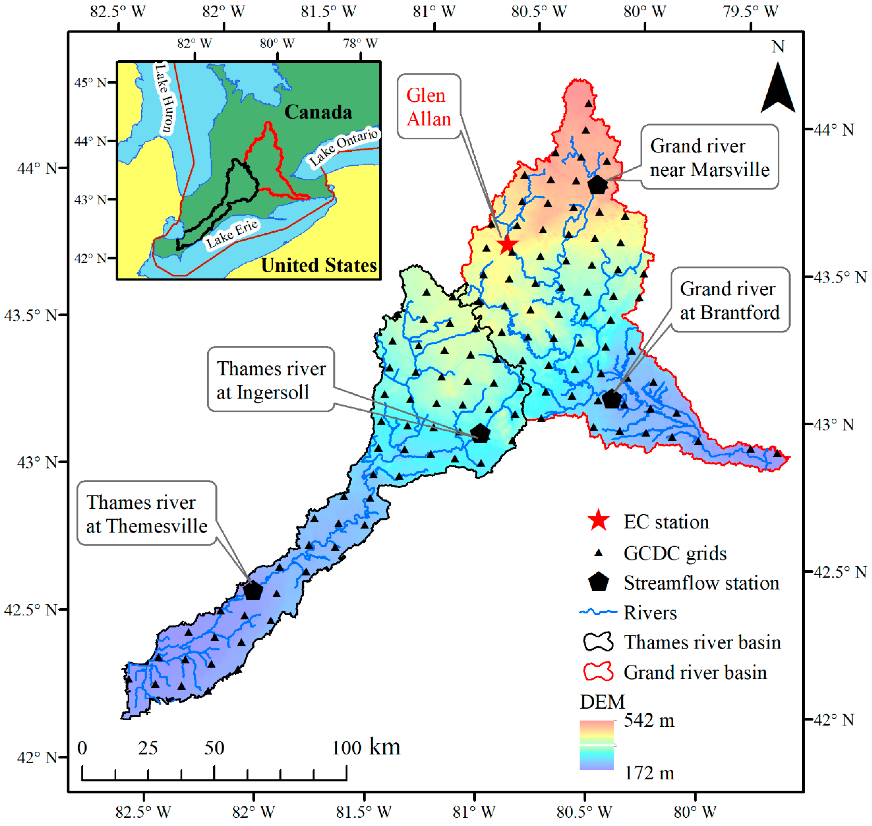
2.1. Study Area
2.2. The Model—Soil and Water Assessment Tool (SWAT)
2.3. Model Build-Up, Inputs, Calibration and Validation
2.4. Model Performance Evaluation
2.5. Future Climate Data
2.6. Bias-Correction Methods
2.6.1. Linear Scaling (LS) of Precipitation and Temperature
2.6.2. Local Intensity Scaling (LOCI) of Precipitation
2.6.3. Power Transformation (PT) of precipitation
2.6.4. Variance Scaling (VS) of temperature
2.6.5. Distribution Mapping (DM) for Precipitation and Temperature
2.7. Evaluation of Bias-Correction Methods
3. Results and Discussion
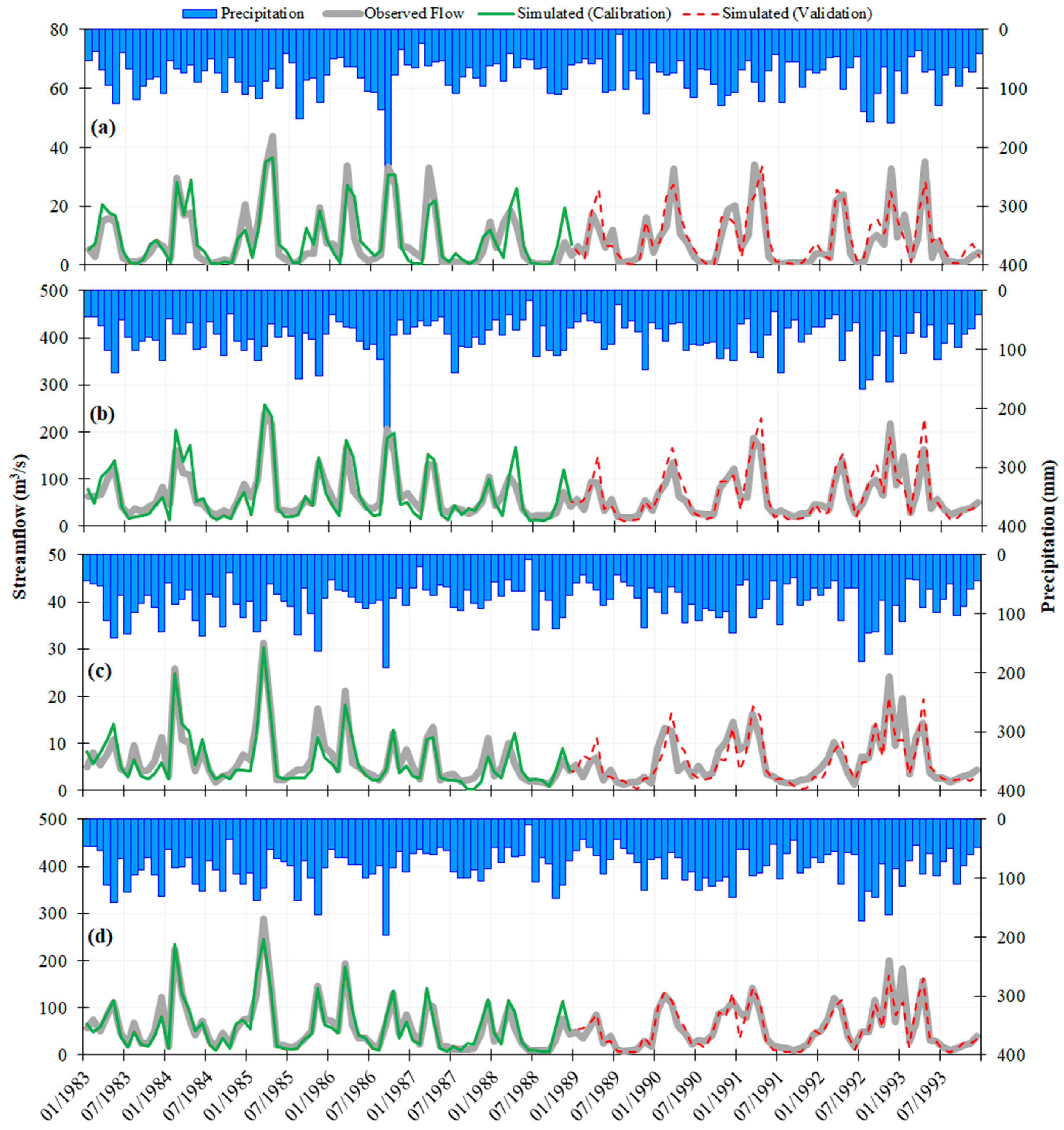
3.1. Streamflow Results in the Base Period
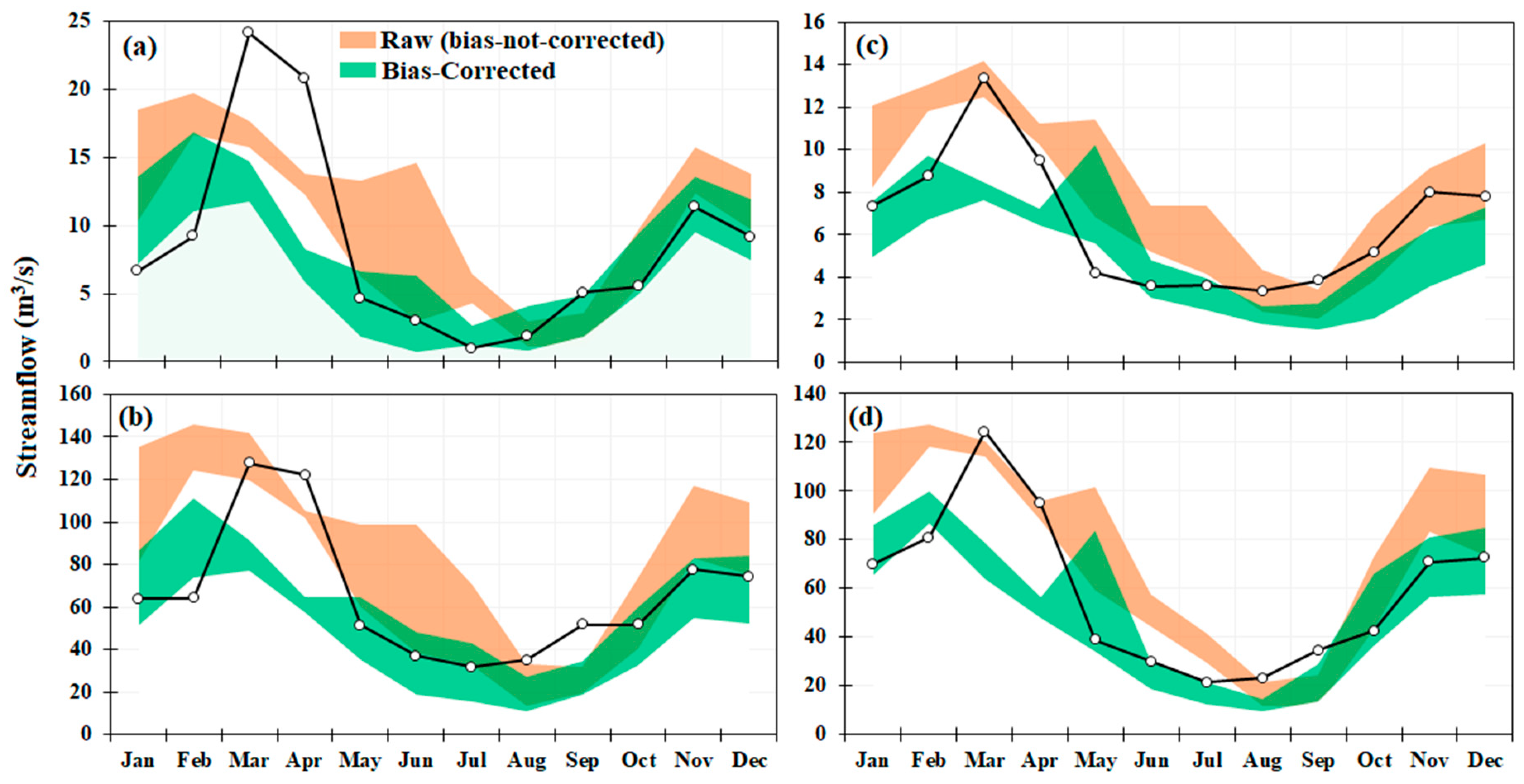
3.2. Performance of Different Bias-Correction Methods
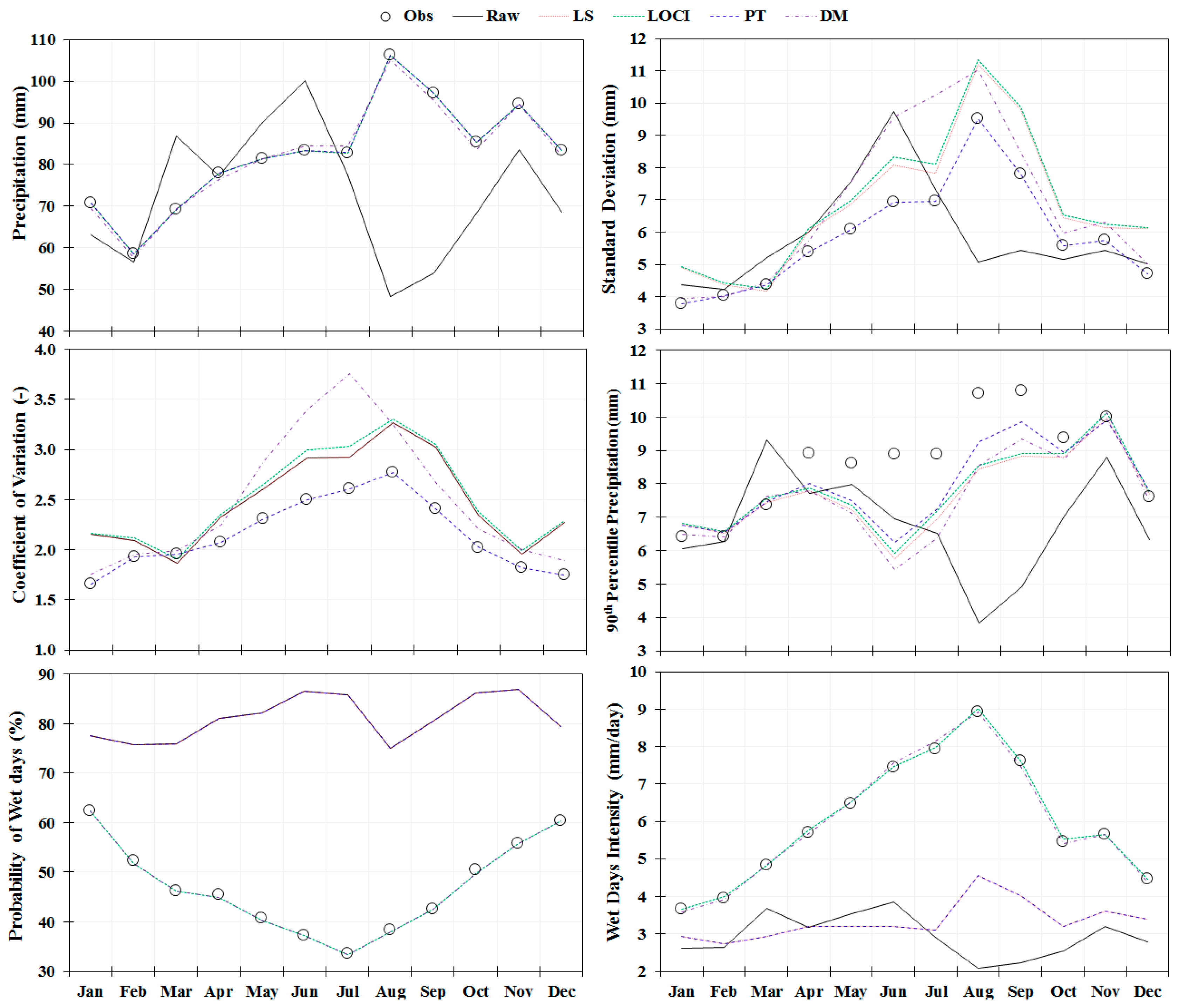
3.2.1. Precipitation
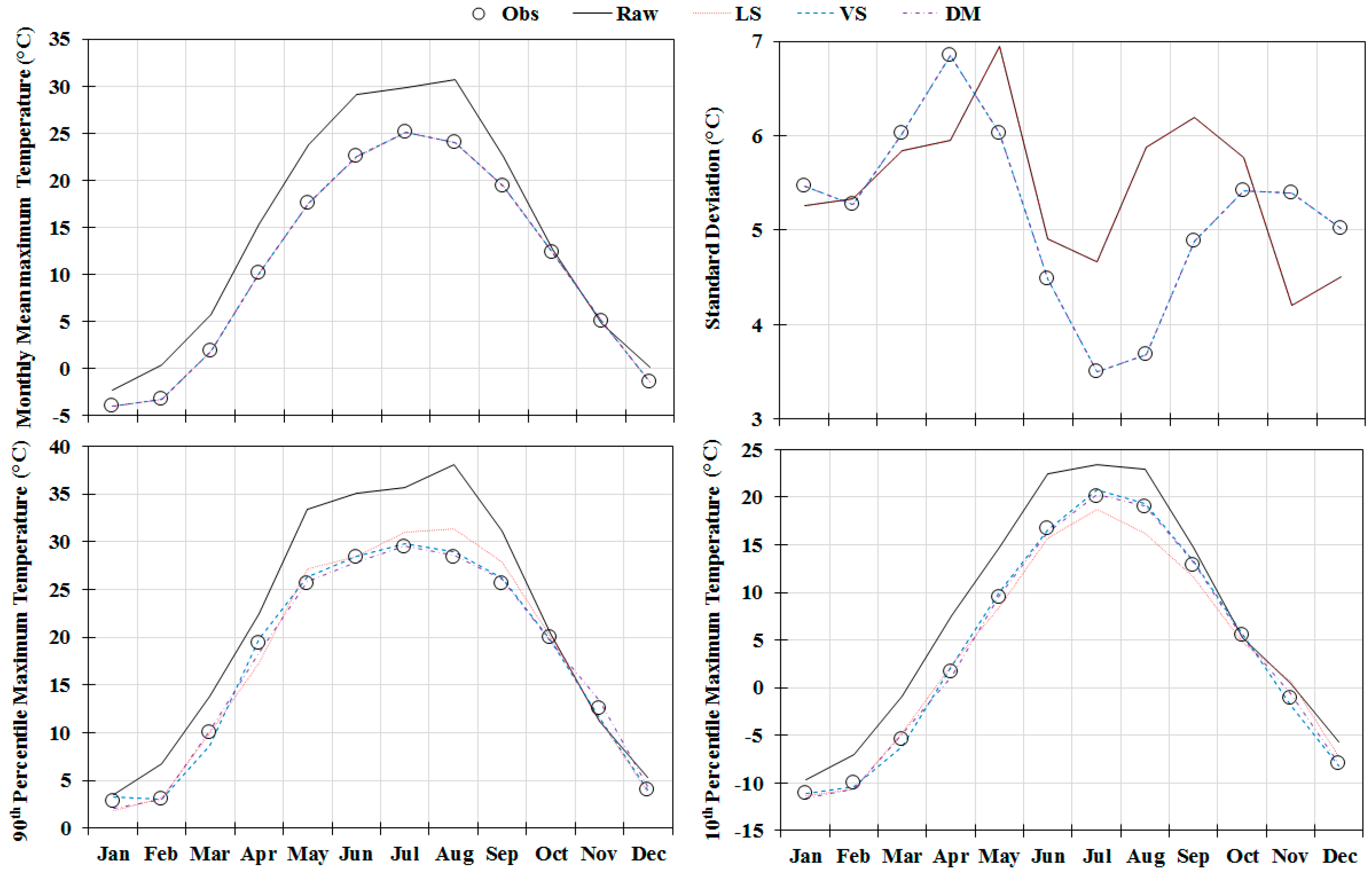
3.2.2. Temperature
3.2.3. Streamflow
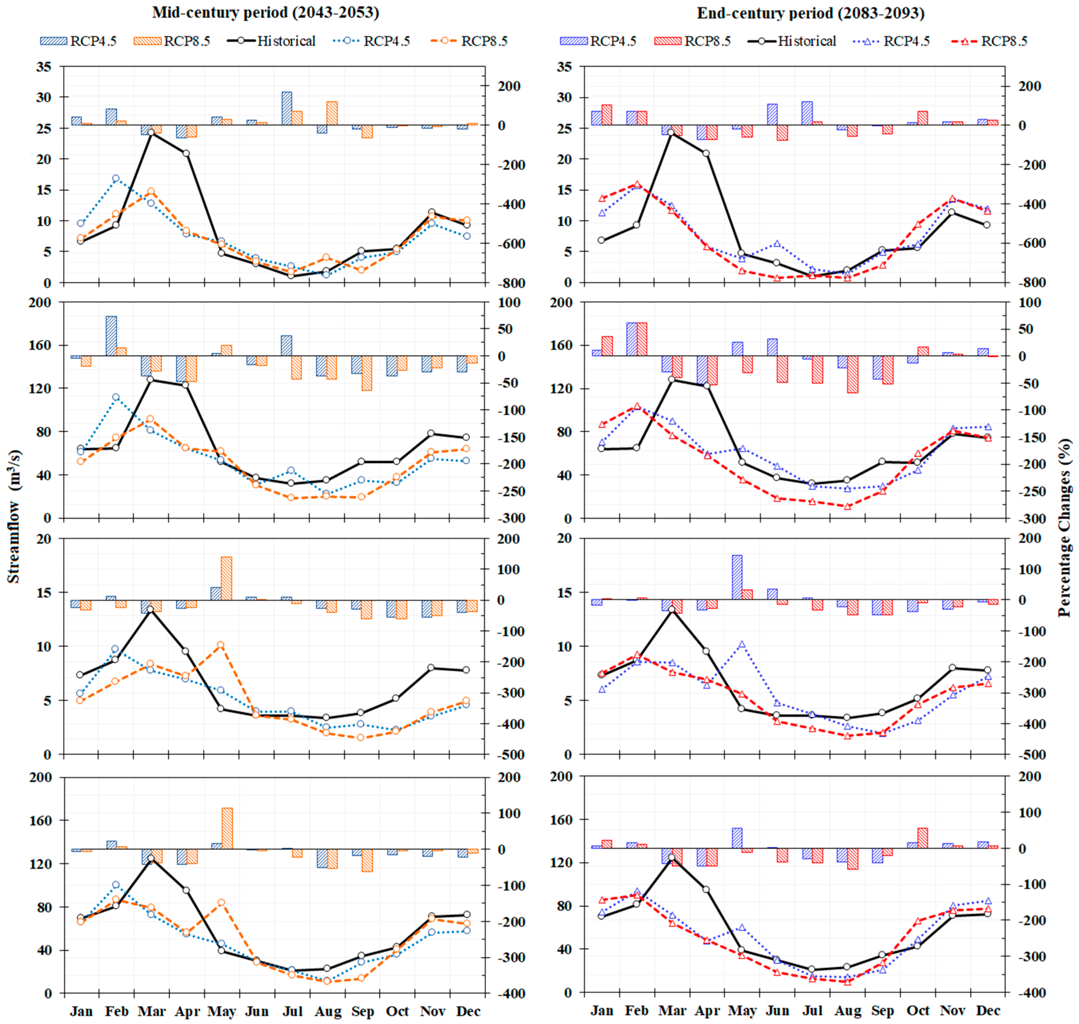
3.3. Streamflow Results in Future Periods
4. Conclusions
Supplementary Materials
Author Contributions
Funding
Acknowledgments
Conflicts of Interest
References
- Sanderson, M. The great-lakes—An environmental atlas and resource book—environment-canada-us-epa-brock-university-northwestern-university. Prof. Geogr. 1988, 40, 250–251. [Google Scholar]
- Makarewicz, J.C.; Bertram, P. Evidence for the restoration of the lake erie ecosystem—Water-quality, oxygen levels, and pelagic function appear to be improving. Bioscience 1991, 41, 216–223. [Google Scholar] [CrossRef]
- Paerl, H.W.; Hall, N.S.; Calandrino, E.S. Controlling harmful cyanobacterial blooms in a world experiencing anthropogenic and climatic-induced change. Sci. Total Environ. 2011, 409, 1739–1745. [Google Scholar] [CrossRef] [PubMed]
- Michalak, A.M.; Anderson, E.J.; Beletsky, D.; Boland, S.; Bosch, N.S.; Bridgeman, T.B.; Chaffin, J.D.; Cho, K.; Confesor, R.; Daloglu, I.; et al. Record-setting algal bloom in lake erie caused by agricultural and meteorological trends consistent with expected future conditions. Proc. Natl. Acad. Sci. USA 2013, 110, 6448–6452. [Google Scholar] [CrossRef] [PubMed]
- Smith, D.; King, K.; Williams, M. What is causing the harmful algal blooms in lake erie? J. Soil Water Conserv. 2015, 70, 27–29. [Google Scholar] [CrossRef]
- Mortsch, L.D.; Quinn, F.H. Climate change scenarios for great lakes basin ecosystem studies. Limnol. Oceanogr. 1996, 41, 903–911. [Google Scholar] [CrossRef]
- Mekis, E.; Hogg, W.D. Rehabilitation and analysis of canadian daily precipitation time series. Atmosphere-Ocean 1999, 37, 53–85. [Google Scholar] [CrossRef]
- Uniyal, B.; Jha, M.; Verma, A. Assessing climate change impact on water balance components of a river basin using swat model. Water Resour. Manag. 2015, 29, 4767–4785. [Google Scholar] [CrossRef]
- Cherkauer, K.A.; Sinha, T. Hydrologic impacts of projected future climate change in the lake michigan region. J. Great Lakes Res. 2010, 36, 33–50. [Google Scholar] [CrossRef]
- Newham, L.T.H.; Letcher, R.A.; Jakeman, A.J.; Kobayashi, T. A framework for integrated hydrologic, sediment and nutrient export modelling for catchment-scale management. Environ. Model. Softw. 2004, 19, 1029–1038. [Google Scholar] [CrossRef]
- Bosch, N.S.; Evans, M.A.; Scavia, D.; Allan, J.D. Interacting effects of climate change and agricultural bmps on nutrient runoff entering lake erie. J. Great Lakes Res. 2014, 40, 581–589. [Google Scholar] [CrossRef]
- Culbertson, A.M.; Martin, J.F.; Aloysius, N.; Ludsin, S.A. Anticipated impacts of climate change on 21st century maumee river discharge and nutrient loads. J. Great Lakes Res. 2016, 42, 1332–1342. [Google Scholar] [CrossRef]
- Verma, S.; Bhattarai, R.; Bosch Nathan, S.; Cooke Richard, C.; Kalita Prasanta, K.; Markus, M. Climate change impacts on flow, sediment and nutrient export in a great lakes watershed using swat. CLEAN—Soil Air Water 2015, 43, 1464–1474. [Google Scholar] [CrossRef]
- Li, Z.; Huang, G.; Wang, X.; Han, J.; Fan, Y. Impacts of future climate change on river discharge based on hydrological inference: A case study of the grand river watershed in Ontario, Canada. Sci. Total Environ. 2016, 548–549, 198–210. [Google Scholar] [CrossRef] [PubMed]
- Arnold, J.G.; Srinivasan, R.; Muttiah, R.S.; Williams, J.R. Large area hydrologic modeling and assessment part I: Model development. J. Am. Water Resour. Assoc. 1998, 34, 73–89. [Google Scholar] [CrossRef]
- Scinocca, J.F.; Kharin, V.V.; Jiao, Y.; Qian, M.W.; Lazare, M.; Solheim, L.; Flato, G.M.; Biner, S.; Desgagne, M.; Dugas, B. Coordinated global and regional climate modeling. J. Clim. 2016, 29, 17–35. [Google Scholar] [CrossRef]
- Rathjens, H.; Bieger, B.; Srinivasan, S.; Chaubey, I.; Arnold, J.G. CMhyd User Manual. Available online: http://swat.tamu.edu/software/cmhyd/ (accessed on 20 February 2018).
- Intergovernmental Panel on Climate Change. Climate Change 2014: Synthesis Report. Contribution of Working Groups I, II and III to the Fifth Assessment Report of the Intergovernmental Panel on Climate Change; IPCC: Geneva, Switzerland, 2014; p. 151. [Google Scholar]
- Daily 10 km Gridded Climate Dataset: 1961–2003, version 1.0; computer file; Agriculture and Agri-Food Canada (AAFC): Ottawa, ON, Canada, 2007.
- Grand River Watershed Characterization Report; Lake Erie Source Protection Region Technical Team: Ontario, Canada, 2008.
- Farwell, J.; Boyd, D.; Ryan, T. Making watersheds more resilient to climate change: A response in the grand river watershed, Ontario Canada. In Proceedings of the 11th Annual River symposium, Brisbane, Australia, 18–20 September 2008. [Google Scholar]
- Goyal, M.K.; Burn, D.H.; Ojha, C.S.P. Evaluation of machine learning tools as a statistical downscaling tool: Temperatures projections for multi-stations for thames river basin, Canada. Theor. Appl. Climatol. 2012, 108, 519–534. [Google Scholar] [CrossRef]
- Prodanovic, P.; Simonovic, S.P. Inverse Flood Risk Modelling of the Upper Thames River Basin. Water Resources Research Report. Available online: https://ir.Lib.Uwo.Ca/wrrr/12 (accessed on 20 February 2018) .
- Arnold, J.G.; Moriasi, D.N.; Gassman, P.W.; Abbaspour, K.C.; White, M.J.; Srinivasan, R.; Santhi, C.; Harmel, R.D.; van Griensven, A.; Van Liew, M.W.; et al. Swat: Model use, calibration, and validation. Trans. ASABE 2012, 55, 1491–1508. [Google Scholar] [CrossRef]
- Shrestha, N.K.; Du, X.; Wang, J. Assessing climate change impacts on fresh water resources of the athabasca river basin, Canada. Sci. Total Environ. 2017, 601–602, 425–440. [Google Scholar] [CrossRef] [PubMed]
- Shrestha, N.K.; Wang, J. Predicting sediment yield and transport dynamics of a cold climate region watershed in changing climate. Sci. Total Environ. 2018, 625, 1030–1045. [Google Scholar] [CrossRef] [PubMed]
- Ahl, R.S.; Woods, S.W.; Zuuring, H.R. Hydrologic calibration and validation of swat in a snow-dominated rocky mountain watershed, montana, U.S.A. 1. JAWRA J. Am. Water Resour. Assoc. 2008, 44, 1411–1430. [Google Scholar] [CrossRef]
- Grusson, Y.; Sun, X.; Gascoin, S.; Sauvage, S.; Raghavan, S.; Anctil, F.; Sáchez-Pérez, J.-M. Assessing the capability of the swat model to simulate snow, snow melt and streamflow dynamics over an alpine watershed. J. Hydrol. 2015, 531, 574–588. [Google Scholar] [CrossRef]
- Faramarzi, M.; Srinivasan, R.; Iravani, M.; Bladon, K.D.; Abbaspour, K.C.; Zehnder, A.J.B.; Goss, G.G. Setting up a hydrological model of alberta: Data discrimination analyses prior to calibration. Environ. Model. Softw. 2015, 74, 48–65. [Google Scholar] [CrossRef]
- Troin, M.; Caya, D. Evaluating the swat’s snow hydrology over a northern quebec watershed. Hydrol. Process. 2014, 28, 1858–1873. [Google Scholar] [CrossRef]
- Malagò, A.; Pagliero, L.; Bouraoui, F.; Franchini, M. Comparing calibrated parameter sets of the swat model for the scandinavian and iberian peninsulas. Hydrol. Sci. J. 2015, 60, 949–967. [Google Scholar] [CrossRef]
- Winchell, M.; Srinivasan, R.; Luzio, M.D. Arcswat Interface for Swat2009 User’s Guide; Soil and Water Research Laboratory—Agricultural Research Service: Blackland, TX, USA, 2010. [Google Scholar]
- Provincial Digital Elevation Model, version 3.0; Ontario Ministry Of Natural Resources And Forestry: Peterborough, ON, Canada, 2015.
- Moriasi, D.N.; Gitau, M.W.; Pai, N.; Daggupati, P. Hydrologic and water quality models: Performance measures and evaluation criteria. Trans. ASABE 2015, 58, 1763–1785. [Google Scholar]
- Nash, J.E.; Sutcliffe, J.V. River flow forecasting through conceptual models part I—A discussion of principles. J. Hydrol. 1970, 10, 282–290. [Google Scholar] [CrossRef]
- Shrestha, N.K.; Leta, O.T.; De Fraine, B.; van Griensven, A.; Bauwens, W. Openmi-based integrated sediment transport modelling of the river zenne, Belgium. Environ. Model. Softw. 2013, 47, 193–206. [Google Scholar] [CrossRef]
- Shrestha, N.K.; Leta, O.T.; Bauwens, W. Development of rwqm1-based integrated water quality model in openmi with application to the river zenne, belgium. Hydrol. Sci. J. 2017, 62, 774–799. [Google Scholar] [CrossRef]
- Von Salzen, K.; Scinocca, J.F.; McFarlane, N.A.; Li, J.N.; Cole, J.N.S.; Plummer, D.; Verseghy, D.; Reader, M.C.; Ma, X.Y.; Lazare, M.; et al. The canadian fourth generation atmospheric global climate model (canam4). Part I: Representation of physical processes. Atmos Ocean 2013, 51, 104–125. [Google Scholar] [CrossRef]
- Hawkins, E.; Sutton, R. The potential to narrow uncertainty in regional climate predictions. Bull. Am. Meteorol. Soc. 2009, 90, 1095–1108. [Google Scholar] [CrossRef]
- Cheng, G.H.; Huang, G.H.; Dong, C.; Zhu, J.X.; Zhou, X.; Yao, Y. An evaluation of cmip5 gcm simulations over the Athabasca river basin, Canada. River Res. Appl. 2017, 33, 823–843. [Google Scholar] [CrossRef]
- Murdock, T.Q.; Cannon, A.J.; Sobie, S.R. Statistical Downscaling of Future Climate Projections; Pacific Climate Impacts Consortium (PCIC): Victoria, British Columbia, Canada, 2013. [Google Scholar]
- Shukla, R.; Khare, P.D.; Deo, R. Statistical downscaling of climate change scenarios of rainfall and temperature over indira sagar canal command area in madhya pradesh, India. In Proceedings of the2015 IEEE 14th International Conference on Machine Learning and Applications (ICMLA), Miami, FL, USA, 9–11 December 2015; pp. 313–317. [Google Scholar]
- Lenderink, G.; Buishand, A.; van Deursen, W. Estimates of future discharges of the river rhine using two scenario methodologies: Direct versus delta approach. Hydrol. Earth Syst. Sci. 2007, 11, 1145–1159. [Google Scholar] [CrossRef]
- Berg, P.; Feldmann, H.; Panitz, H.J. Bias correction of high resolution regional climate model data. J. Hydrol. 2012, 448, 80–92. [Google Scholar] [CrossRef]
- Olsson, T.; Jakkila, J.; Veijalainen, N.; Backman, L.; Kaurola, J.; Vehvilainen, B. Impacts of climate change on temperature, precipitation and hydrology in finland—Studies using bias corrected regional climate model data. Hydrol. Earth Syst. Sci. 2015, 19, 3217–3238. [Google Scholar] [CrossRef]
- Schmidli, J.; Frei, C.; Vidale, P.L. Downscaling from gc precipitation: A benchmark for dynamical and statistical downscaling methods. Int. J. Climatol. 2006, 26, 679–689. [Google Scholar] [CrossRef]
- Teutschbein, C.; Seibert, J. Bias correction of regional climate model simulations for hydrological climate-change impact studies: Review and evaluation of different methods. J. Hydrol. 2012, 456, 12–29. [Google Scholar] [CrossRef]
- Fang, G.H.; Yang, J.; Chen, Y.N.; Zammit, C. Comparing bias correction methods in downscaling meteorological variables for a hydrologic impact study in an arid area in china. Hydrol. Earth Syst. Sci. 2015, 19, 2547–2559. [Google Scholar] [CrossRef]
- Leander, R.; Buishand, T.A.; van den Hurk, B.J.J.M.; de Wit, M.J.M. Estimated changes in flood quantiles of the river meuse from resampling of regional climate model output. J. Hydrol. 2008, 351, 331–343. [Google Scholar] [CrossRef]
- Terink, W.; Hurkmans, R.T.W.L.; Torfs, P.J.J.F.; Uijlenhoet, R. Evaluation of a bias correction method applied to downscaled precipitation and temperature reanalysis data for the rhine basin. Hydrol. Earth Syst. Sci. 2010, 14, 687–703. [Google Scholar] [CrossRef]
- Mbaye, M.L.; Haensler, A.; Hagemann, S.; Gaye, A.T.; Moseley, C.; Afouda, A. Impact of statistical bias correction on the projected climate change signals of the regional climate model remo over the senegal river basin. Int. J. Climatol. 2016, 36, 2035–2049. [Google Scholar] [CrossRef]
- Tschoke, G.V.; Kruk, N.S.; Queiroz, P.I.B.; Chou, S.; de Sousa, W.C. Comparison of two bias correction methods for precipitation simulated with a regional climate model. Theor. Appl. Climatol. 2017, 127, 841–852. [Google Scholar] [CrossRef]
- Falkenmark, M.; Rockström, J. The new blue and green water paradigm: Breaking new ground for water resources planning and management. J. Water Resour. Plan. Manag. 2006, 132, 129–132. [Google Scholar] [CrossRef]
- Eum, H.-I.; Dibike, Y.; Prowse, T. Climate-induced alteration of hydrologic indicators in the athabasca river basin, alberta, Canada. J. Hydrol. 2017, 544, 327–342. [Google Scholar] [CrossRef]
- Toth, B.; Pietroniro, A.; Conly, F.M.; Kouwen, N. Modelling climate change impacts in the peace and athabasca catchment and delta: I—Hydrological model application. Hydrol. Process. 2006, 20, 4197–4214. [Google Scholar] [CrossRef]
- Choi, W.; Kim, S.J.; Lee, M.; Koenig, K.; Rasmussen, P. Hydrological impacts of warmer and wetter climate in troutlake and sturgeon river basins in central canada. Water Resour. Manag. 2014, 28, 5319–5333. [Google Scholar] [CrossRef]
- Rahman, M.; Bolisetti, T.; Balachandar, R. Effect of climate change on low-flow conditions in the ruscom river watershed, ontario. Trans. ASABE 2010, 53, 1521–1532. [Google Scholar] [CrossRef]
- Cousino, L.K.; Becker, R.H.; Zmijewski, K.A. Modeling the effects of climate change on water, sediment, and nutrient yields from the maumee river watershed. J. Hydrol. Reg. Stud. 2015, 4, 762–775. [Google Scholar] [CrossRef]
- Basile Samantha, J.; Rauscher Sara, A.; Steiner Allison, L. Projected precipitation changes within the great lakes and western lake erie basin: A multi-model analysis of intensity and seasonality. Int. J. Climatol. 2017, 37, 4864–4879. [Google Scholar] [CrossRef]
- Cohen, J.; Ye, H.; Jones, J. Trends and variability in rain-on-snow events. Geophys. Res. Lett. 2015, 42, 7115–7122. [Google Scholar] [CrossRef]
- Choi, W.; Rasmussen, P.; Moore, A.; Kim, S. Simulating streamflow response to climate scenarios in central canada using a simple statistical downscaling method. Climate Res. 2009, 40, 89–102. [Google Scholar] [CrossRef]
- Shrestha, R.R.; Dibike, Y.B.; Prowse, T.D. Modelling of climate-induced hydrologic changes in the lake winnipeg watershed. J. Great Lakes Res. 2012, 38, 83–94. [Google Scholar] [CrossRef]
- Chien, H.; Yeh, P.J.F.; Knouft, J.H. Modeling the potential impacts of climate change on streamflow in agricultural watersheds of the midwestern united states. J. Hydrol. 2013, 491, 73–88. [Google Scholar] [CrossRef]


| Streamflow Gauging Stations | Calibration | Validation | ||||
|---|---|---|---|---|---|---|
| R2 | PBIAS (%) | NSE | R2 | PBIAS (%) | NSE | |
| Grand river near Marsville | 0.80(G) | –10(S) | 0.78(G) | 0.77(G) | –14(S) | 0.74(G) |
| Grand river at Brantford | 0.88(VG) | –2(VG) | 0.77(G) | 0.83(G) | –7(G) | 0.72(G) |
| Thames river at Ingersoll | 0.85(VG) | 7(G) | 0.84(VG) | 0.75(G) | 5(G) | 0.73(G) |
| Thames river at Thamesville | 0.91(VG) | 1(VG) | 0.91(VG) | 0.88(VG) | 3(VG) | 0.88(VG) |
| VG: Very Good; G: Good; S: Satisfactory; US: Unsatisfactory | ||||||
| R2: Coefficient of determination; PBIAS: Percentage of bias; NSE: Nash-Sutcliffe Efficiency | ||||||
| Statistics | Obs. | Raw | LS | LOCI | PT | DM |
|---|---|---|---|---|---|---|
| Frequency based | ||||||
| Mean (mm) | 2.71 | 2.39 | 2.71 | 2.71 | 2.71 | 2.69 |
| Median (mm) | 0 | 0.21 | 0.24 | 0 | 0.39 | 0 |
| Standard Deviation (mm) | 6.14 | 6.1 | 7.14 | 7.26 | 6.14 | 7.28 |
| Coefficient of Variation (-) | 2.26 | 2.55 | 2.63 | 2.68 | 2.26 | 2.7 |
| 90th Percentile (mm) | 8.6 | 6.89 | 7.57 | 7.69 | 7.81 | 7.5 |
| Probability of Wet Days (%) | 47.12 | 81.1 | 81.1 | 46.89 | 81.1 | 46.89 |
| Intensity of Wet Days (mm/day) | 5.76 | 2.95 | 3.34 | 5.79 | 3.34 | 5.75 |
| Time-series based | ||||||
| Coefficient of Determination - R2 | - | 0.04 | 1 | 1 | 1 | 0.99 |
| Percentage Bias - PBIAS (%) | - | 11.8 | 0.01 | 0 | 0 | 0.69 |
| Nash-Sutcliffe Efficiency - NSE | - | –0.7 | 1 | 1 | 1 | 0.99 |
| Mean Absolute Error - MAE (°C) | - | 16.92 | 0.01 | 0 | 0.01 | 1.08 |
| LS: Linear Scaling; LOCI: Local Internsity Scaling; DM: Distribution Mapping | ||||||
| Statistics | Obs. | Raw | LS | VS | DM |
|---|---|---|---|---|---|
| Frequency based | |||||
| Mean (°C) | 10.83 | 14.47 | 10.83 | 10.83 | 10.83 |
| Median (°C) | 11.1 | 13.92 | 10.71 | 10.93 | 11.42 |
| Standard Deviation (°C) | 11.71 | 13.21 | 11.83 | 11.71 | 11.71 |
| Coefficient of Variation | 1.08 | 0.91 | 1.09 | 1.08 | 1.08 |
| 90th Percentile (°C) | 26 | 32.49 | 26.77 | 26.08 | 26.01 |
| 10th Percentile (°C) | –5 | –1.69 | –4.12 | –4.83 | –4.37 |
| Time-series based | |||||
| Coefficient of Determination - R2 | - | 0.92 | 0.93 | 0.94 | 0.93 |
| Percentage Bias - PBIAS (%) | - | –33.84 | –0.02 | –0.01 | –0.01 |
| Nash-Sutcliffe Efficiency - NSE | - | 0.84 | 0.93 | 0.94 | 0.93 |
| Mean Absolute Error - MAE (°C) | - | 4.23 | 2.31 | 2.05 | 2.2 |
| LS: Linear Scaling; VS: Variance Scaling; DM: Distribution Mapping | |||||
| Simulations/Combinations | Grand River near Marsville | Grand River at Brantford | Thames River at Ingersoll | Thames River at Thamesville | ||||||||
|---|---|---|---|---|---|---|---|---|---|---|---|---|
| R2 | PBIAS (%) | NSE | R2 | PBIAS (%) | NSE | R2 | PBIAS (%) | NSE | R2 | PBIAS (%) | NSE | |
| Baseline | 0.93 | –10.9 | 0.91 | 0.94 | –4.25 | 0.86 | 0.81 | 6.42 | 0.79 | 0.98 | 1.63 | 0.97 |
| Raw | 0.61 | 11.49 | 0.22 | 0.68 | 4.77 | 0.64 | 0.69 | –2.01 | 0.59 | 0.83 | –4.01 | 0.81 |
| P(LS) + T(LS) | 0.68 | –44 | 0.46 | 0.77 | –36.66 | 0.52 | 0.62 | –36.69 | 0.3 | 0.78 | –29.81 | 0.52 |
| P(LS) + T(VS) | 0.67 | –43.36 | 0.4 | 0.76 | –36.6 | 0.51 | 0.62 | –35.99 | 0.25 | 0.83 | –22.07 | 0.56 |
| P(LS) + T(DM) | 0.67 | –43.24 | 0.43 | 0.77 | –36.78 | 0.52 | 0.6 | –36.72 | 0.28 | 0.76 | –29.57 | 0.5 |
| P(LOCI) + T(LS) | 0.73 | –26.7 | 0.6 | 0.83 | –18.86 | 0.73 | 0.67 | –19.95 | 0.48 | 0.86 | –15.35 | 0.75 |
| P(LOCI) + T(VS) | 0.71 | –25.91 | 0.54 | 0.81 | –18.62 | 0.72 | 0.67 | –19.03 | 0.43 | 0.86 | –14.68 | 0.73 |
| P(LOCI) + T(DM) | 0.73 | –25.95 | 0.58 | 0.83 | –18.93 | 0.73 | 0.65 | –19.97 | 0.46 | 0.85 | –15.16 | 0.73 |
| P(PT) + T(LS) | 0.7 | –52.83 | 0.44 | 0.77 | –43.77 | 0.49 | 0.72 | –41.55 | 0.43 | 0.78 | –33.81 | 0.56 |
| P(PT) + T(VS) | 0.69 | –52.39 | 0.39 | 0.77 | –43.92 | 0.48 | 0.74 | –41.11 | 0.41 | 0.77 | –33.37 | 0.54 |
| P(PT) + T(DM) | 0.7 | –52.23 | 0.42 | 0.77 | –43.97 | 0.49 | 0.72 | –41.63 | 0.42 | 0.76 | –33.75 | 0.54 |
| P(DM) + T(LS) | 0.78 | –14 | 0.72 | 0.84 | –6.2 | 0.83 | 0.63 | –7.04 | 0.57 | 0.92 | –4.95 | 0.9 |
| P(DM) + T(VS) | 0.78 | -13.45 | 0.69 | 0.85 | –6.19 | 0.83 | 0.64 | –6.13 | 0.56 | 0.92 | –4.34 | 0.9 |
| P(DM) + T(DM) | 0.79 | –13.44 | 0.72 | 0.85 | –6.48 | 0.84 | 0.63 | –7.07 | 0.58 | 0.91 | –4.9 | 0.89 |
| P: Precipitation; T: Temperature | ||||||||||||
| LS: Linear Scaling; VS: Variance Scaling; DM: Distribution Map; LOCI: Local Intensity Scaling; PT: Power Transformation | ||||||||||||
| Variables | Emission Scenarios/Periods | Jan | Feb | Mar | Apr | May | Jun | Jul | Aug | Sep | Oct | Nov | Dec |
|---|---|---|---|---|---|---|---|---|---|---|---|---|---|
| Precipitation Changes (%) | RCP4.5 Mid-century | –12 | 16 | 11 | 23 | 11 | 6 | –5 | –27 | 0 | 2 | –19 | –15 |
| RCP8.5 Mid-century | –1 | 7 | 15 | 27 | 55 | 4 | –10 | –6 | –21 | 21 | –3 | –23 | |
| RCP4.5 End-century | –6 | 26 | 18 | 32 | 19 | 31 | –40 | –12 | –22 | 31 | –7 | –5 | |
| RCP8.5 End-century | 3 | 38 | 8 | 27 | –11 | 18 | -1 | –27 | -2 | 21 | –16 | 6 | |
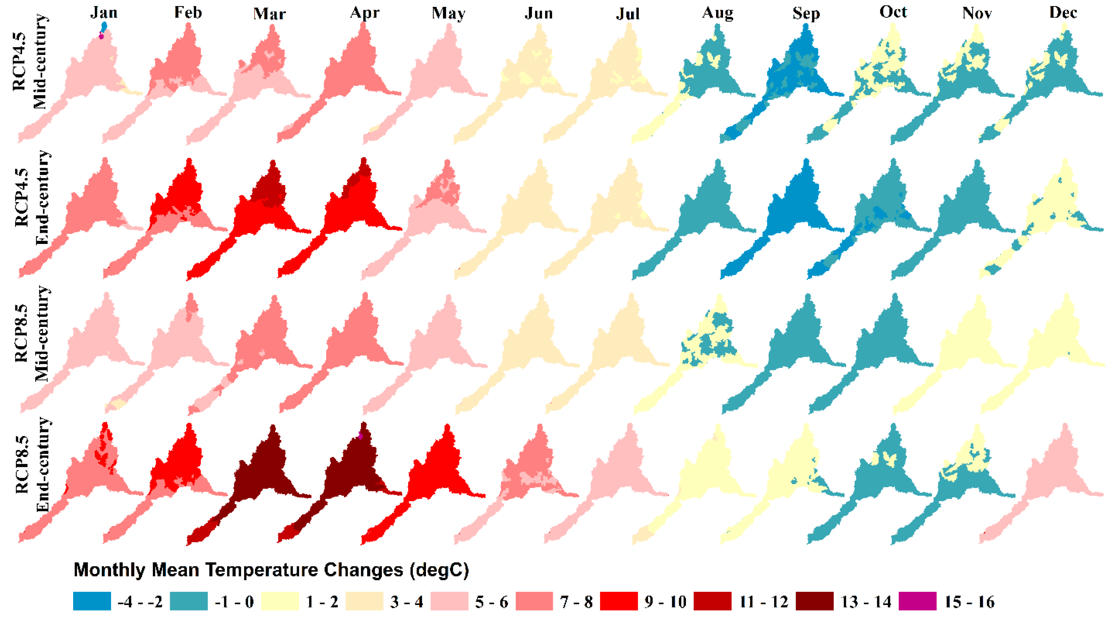
| Average Temperature Changes (°C) | RCP4.5 Mid-century | 4.5 | 5.8 | 5.6 | 6.5 | 4.5 | 2.4 | 2.5 | 0.2 | –2.0 | –0.1 | –0.3 | –0.1 |
| RCP8.5 Mid-century | 4.6 | 4.7 | 6.3 | 6.5 | 5.2 | 3.3 | 3.0 | 0.4 | –0.7 | –0.8 | 0.5 | 0.8 | |
| RCP4.5 End-century | 6.7 | 7.7 | 9.4 | 9.2 | 5.9 | 3.1 | 2.9 | –0.7 | –2.8 | –1.9 | –0.8 | 0.3 | |
| RCP8.5 End-century | 7.8 | 7.9 | 12.4 | 12.5 | 8.8 | 6.1 | 5.6 | 2.0 | 0.4 | –0.4 | –0.2 | 5.6 | |
| Green Water Flow Changes (%) | RCP4.5 Mid-century | 125 | 128 | 58 | 39 | 38 | 9 | –12 | –26 | –23 | –8 | 15 | 10 |
| RCP8.5 Mid-century | 123 | 119 | 55 | 36 | 42 | 7 | –11 | –23 | –12 | –12 | 18 | 19 | |
| RCP4.5 End-century | 170 | 157 | 73 | 54 | 51 | 5 | –22 | –39 | –23 | –12 | 10 | 15 | |
| RCP8.5 End-century | 188 | 173 | 88 | 70 | 53 | 1 | –16 | –48 | –34 | –15 | 9 | 56 | |
| Green Water Storage Changes (%) | RCP4.5 Mid-century | –15 | –21 | –10 | –3 | –22 | -35 | –37 | –33 | –4 | 5 | –4 | 1 |
| RCP8.5 Mid-century | –15 | –19 | –12 | –2 | –21 | -35 | –40 | –12 | –12 | 9 | 0 | –9 | |
| RCP4.5 End-century | –19 | –23 | –15 | –3 | –34 | -30 | –52 | –9 | –9 | 14 | –1 | –1 | |
| RCP8.5 End-century | –20 | –22 | –20 | –19 | –56 | -50 | –37 | –6 | 12 | 12 | –4 | –9 |
© 2018 by the authors. Licensee MDPI, Basel, Switzerland. This article is an open access article distributed under the terms and conditions of the Creative Commons Attribution (CC BY) license (http://creativecommons.org/licenses/by/4.0/).
Share and Cite
Zhang, B.; Shrestha, N.K.; Daggupati, P.; Rudra, R.; Shukla, R.; Kaur, B.; Hou, J. Quantifying the Impacts of Climate Change on Streamflow Dynamics of Two Major Rivers of the Northern Lake Erie Basin in Canada. Sustainability 2018, 10, 2897. https://doi.org/10.3390/su10082897
Zhang B, Shrestha NK, Daggupati P, Rudra R, Shukla R, Kaur B, Hou J. Quantifying the Impacts of Climate Change on Streamflow Dynamics of Two Major Rivers of the Northern Lake Erie Basin in Canada. Sustainability. 2018; 10(8):2897. https://doi.org/10.3390/su10082897
Chicago/Turabian StyleZhang, Binbin, Narayan Kumar Shrestha, Prasad Daggupati, Ramesh Rudra, Rituraj Shukla, Baljeet Kaur, and Jun Hou. 2018. "Quantifying the Impacts of Climate Change on Streamflow Dynamics of Two Major Rivers of the Northern Lake Erie Basin in Canada" Sustainability 10, no. 8: 2897. https://doi.org/10.3390/su10082897
APA StyleZhang, B., Shrestha, N. K., Daggupati, P., Rudra, R., Shukla, R., Kaur, B., & Hou, J. (2018). Quantifying the Impacts of Climate Change on Streamflow Dynamics of Two Major Rivers of the Northern Lake Erie Basin in Canada. Sustainability, 10(8), 2897. https://doi.org/10.3390/su10082897