A Statistical Tool to Detect and Locate Abnormal Operating Conditions in Photovoltaic Systems


Abstract
1. Introduction
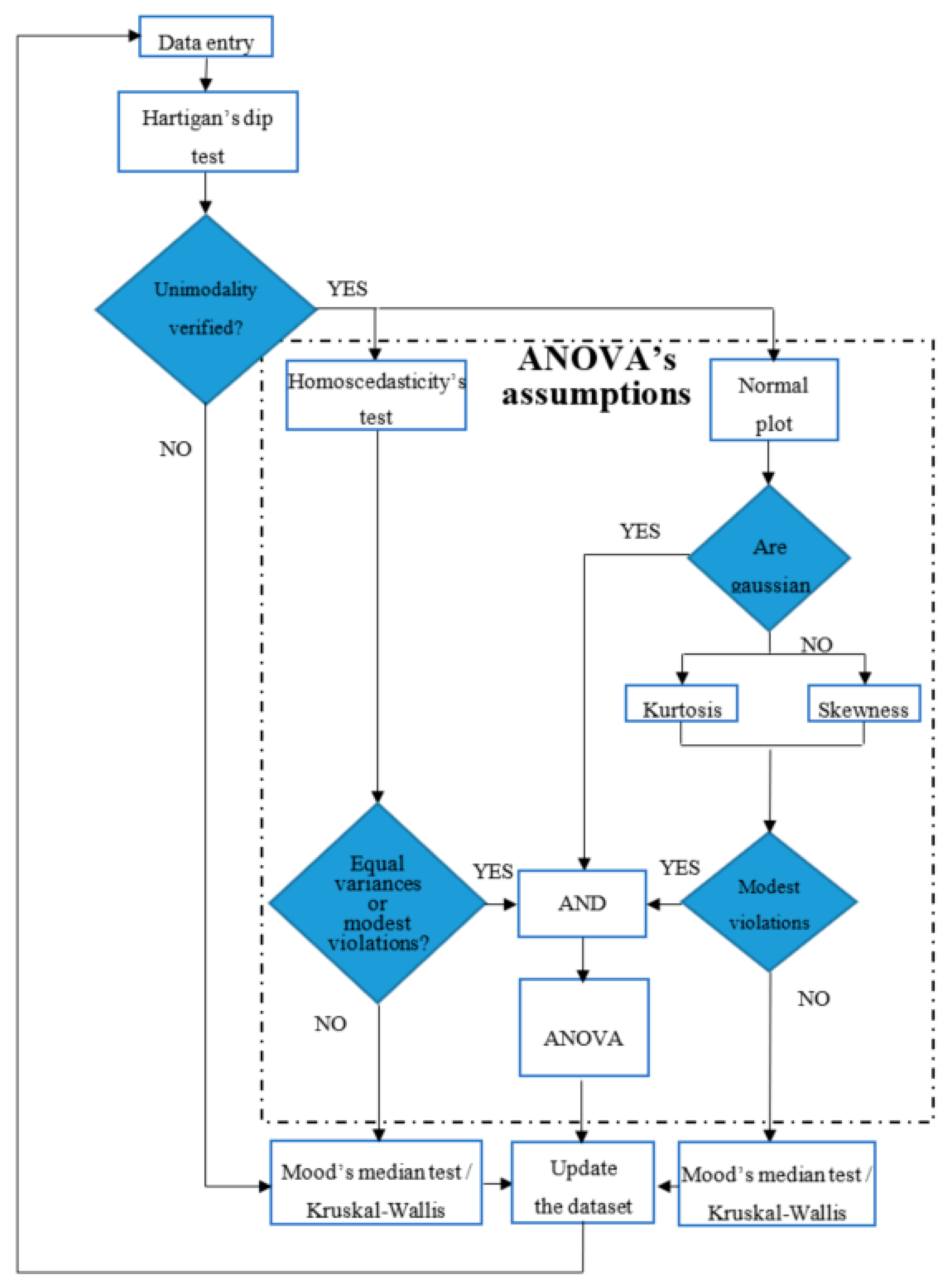
2. Statistical Methodology
- (a)
- all the observations are mutually independent;
- (b)
- all the distributions have equal variance; and,
- (c)
- all the distributions are normally distributed.
3. Description of the PV Plant under Investigation
4. Cumulative Statistical Analysis
- one-month analysis (January);
- six-months analysis (January–June); and,
- one-year analysis (January–December).
4.1. One-Month Analysis (January)
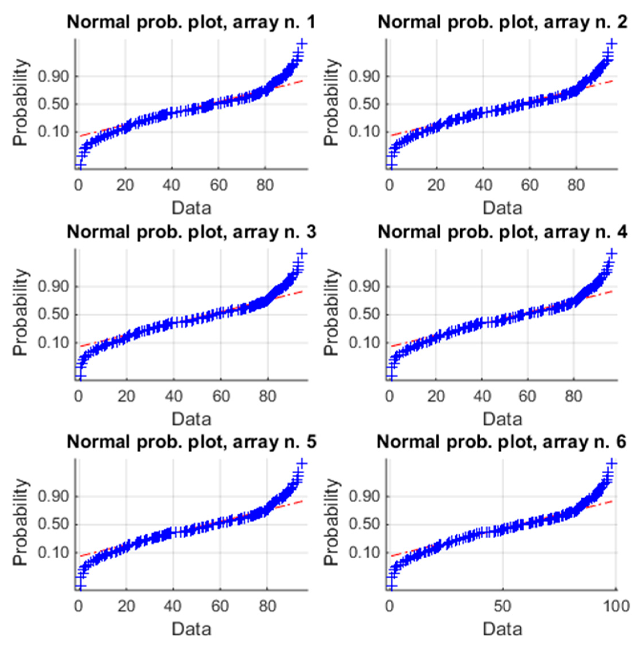
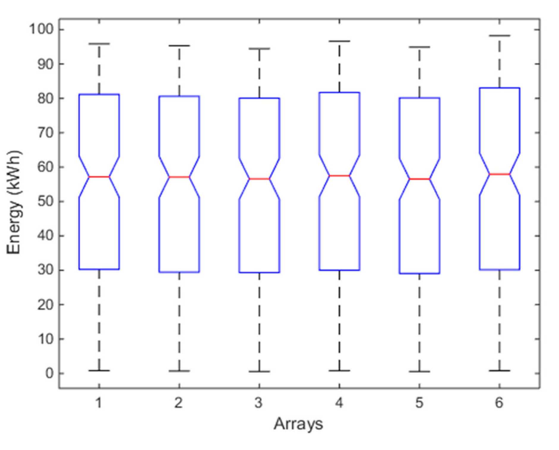
4.2. Six-Months Analysis (January–June)
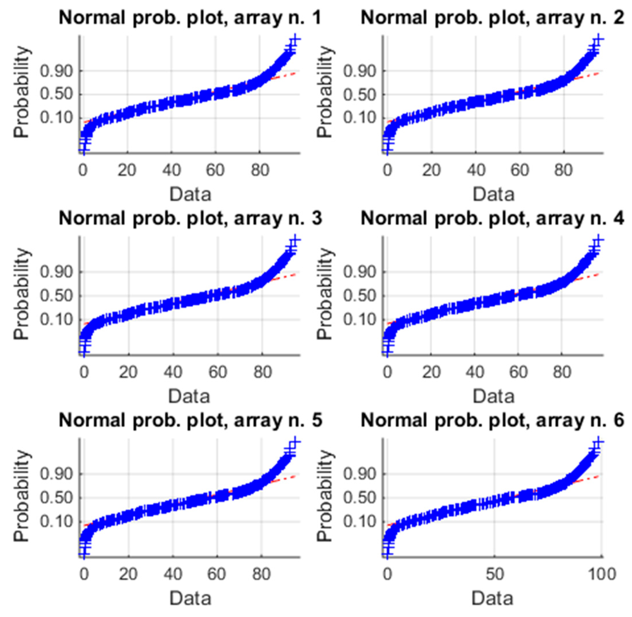
4.3. One-Year Analysis (January–December)
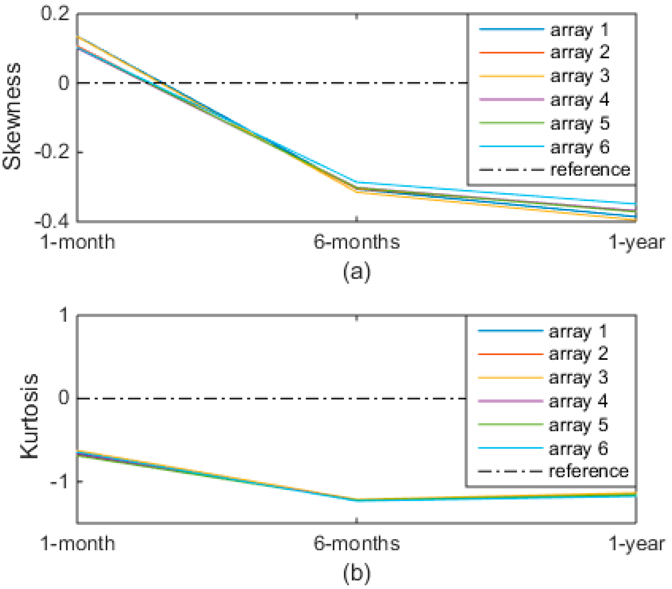
4.4. Discussion
5. Conclusions
Conflicts of Interest
References
- Grimaccia, F.; Leva, S.; Mussetta, M.; Ogliari, E. ANN sizing procedure for the day-ahead output power forecast of a PV plant. Appl. Sci. 2017, 7, 622. [Google Scholar] [CrossRef]
- Massi Pavan, A.; Vergura, S.; Mellit, A.; Lughi, V. Explicit empirical model for photovoltaic devices. Experimental validation. Sol. Energy 2017, 155, 647–653. [Google Scholar] [CrossRef]
- Dellino, G.; Laudadio, T.; Mari, R.; Mastronardi, N.; Meloni, C.; Vergura, S. Energy Production Forecasting in a PV Plant Using Transfer Function Models. In Proceedings of the 2015 IEEE 15th International Conference on Environment and Electrical Engineering (EEEIC), Rome, Italy, 10–13 June 2015. [Google Scholar]
- Guerriero, P.; Di Napoli, F.; Vallone, G.; D’Alessandro, V.; Daliento, S. Monitoring and diagnostics of PV plants by a wireless self-powered sensor for individual panels. IEEE J. Photovolt. 2015, 6, 286–294. [Google Scholar] [CrossRef]
- Johnston, S.; Guthrey, H.; Yan, F.; Zaunbrecher, K.; Al-Jassim, M.; Rakotoniaina, P.; Kaes, M. Correlating multicrystalline silicon defect types using photoluminescence, defect-band emission, and lock-in thermography imaging techniques. IEEE J. Photovolt. 2014, 4, 348–354. [Google Scholar] [CrossRef]
- Peloso, M.; Meng, L.; Bhatia, C.S. Combined thermography and luminescence imaging to characterize the spatial performance of multicrystalline Si wafer solar cells. IEEE J. Photovolt. 2015, 5, 102–111. [Google Scholar] [CrossRef]
- Vergura, S.; Marino, F. Quantitative and computer aided thermography-based diagnostics for PV devices: Part I—Framework. IEEE J. Photovolt. 2017, 7, 822–827. [Google Scholar] [CrossRef]
- Vergura, S.; Colaprico, M.; de Ruvo, M.F.; Marino, F. A quantitative and computer aided thermography-based diagnostics for PV devices: Part II—Platform and results. IEEE J. Photovolt. 2017, 7, 237–243. [Google Scholar] [CrossRef]
- Mekki, H.; Mellit, A.; Salhi, H. Artificial neural network-based modelling and fault detection of partial shaded photovoltaic modules. Simul. Model. Pract. Theory 2016, 67, 1–13. [Google Scholar] [CrossRef]
- Vergura, S. Scalable Model of PV Cell in Variable Environment Condition Based on the Manufacturer Datasheet for Circuit Simulation. In Proceedings of the 2015 IEEE 15th International Conference on Environment and Electrical Engineering (EEEIC), Rome, Italy, 10–13 June 2015. [Google Scholar]
- Harrou, F.; Sun, Y.; Kara, K.; Chouder, A.; Silvestre, S.; Garoudja, E. Statistical fault detection in photovoltaic systems. Sol. Energy 2017, 150, 485–499. [Google Scholar]
- Vergura, S.; Carpentieri, M. Statistics to detect low-intensity anomalies in PV systems. Energies 2018, 11, 30. [Google Scholar] [CrossRef]
- Ventura, C.; Tina, G.M. Development of models for on line diagnostic and energy assessment analysis of PV power plants: The study case of 1 MW Sicilian PV plant. Energy Procedia 2015, 83, 248–257. [Google Scholar] [CrossRef]
- Il-Song, K. On-line fault detection algorithm of a photovoltaic system using wavelet transform. Sol. Energy 2016, 226, 137–145. [Google Scholar]
- Rabhia, A.; El hajjajia, A.; Tinab, M.H.; Alia, G.M. Real time fault detection in photovoltaic systems. Energy Procedia 2017, 11, 914–923. [Google Scholar]
- Plato, R.; Martel, J.; Woodruff, N.; Chau, T.Y. Online fault detection in PV systems. IEEE Trans. Sustain. Energy 2015, 6, 1200–1207. [Google Scholar] [CrossRef]
- Ando, B.; Bagalio, A.; Pistorio, A. Sentinella: Smart monitoring of photovoltaic systems at panel level. IEEE Trans. Instrum. Meas. 2015, 64, 2188–2199. [Google Scholar] [CrossRef]
- IEC International Standard 61724—Photovoltaic System Performance Monitoring—Guidelines for Measurement, Data Exchange and Analysis; International Electrotechnical Commission: Geneva, Switzerland, 1998.
- Leloux, J.; Narvarte, L.; Trebosc, D. Review of the performance of residential PV systems in Belgium. Renew. Sustain. Energy Rev. 2012, 16, 178–184. [Google Scholar] [CrossRef]
- Leloux, J.; Narvarte, L.; Trebosc, D. Review of the performance of residential PV systems in France. Renew. Sustain. Energy Rev. 2012, 16, 1369–1376. [Google Scholar] [CrossRef]
- Hogg, R.V.; Ledolter, J. Engineering Statistics; MacMillan: Basingstoke, UK, 1987. [Google Scholar]
- Hartigan, J.A.; Hartigan, P.M. The dip test of unimodality. Ann. Stat. 1985, 13, 70–84. [Google Scholar] [CrossRef]
- Rohatgi, V.K.; Szekely, G.J. Sharp inequalities between skewness and kurtosis. Stat. Probab. Lett. 1989, 8, 297–299. [Google Scholar] [CrossRef]
- Klaassen, C.A.J.; Mokveld, P.J.; van Es, B. Squared skewness minus kurtosis bounded by 186/125 for unimodal distributions. Stat. Probab. Lett. 2000, 50, 131–135. [Google Scholar] [CrossRef]
- Gibbons, J.D. Nonparametric Statistical Inference, 2nd ed.; M. Dekker: New York, NY, USA, 1985. [Google Scholar]
- Hollander, M.; Wolfe, D.A. Nonparametric Statistical Methods; Wiley: Hoboken, NJ, USA, 1973. [Google Scholar]
- Chambers, J.; Cleveland, W.; Kleiner, B.; Tukey, P. Graphical Methods for Data Analysis; Wadsworth: Belmont, CA, USA, 1983. [Google Scholar]
- Gravetter, F.; Wallnau, L. Essentials of Statistics for the Behavioral Sciences, 8th ed.; Wadsworth: Belmont, CA, USA, 2014. [Google Scholar]
- Tabachnick, B.G.; Fidell, L.S. Using Multivariate Statistics, 6th ed.; Pearson: London, UK, 2013. [Google Scholar]
- George, D.; Mallery, P. SPSS for Windows Step by Step. A Simple Guide and Reference 17.0 Update, 10th ed.; Pearson: Boston, MA, USA, 2010. [Google Scholar]
- PVGIS. Available online: http://re.jrc.ec.europa.eu/pvg_tools/en/tools.html (accessed on 25 February 2018).


| Array Number | ||||||
|---|---|---|---|---|---|---|
| Parameter | 1 | 2 | 3 | 4 | 5 | 6 |
| p-value (HDT) | 0.534 | 0.678 | 0.418 | 0.624 | 0.624 | 0.648 |
| p-value (HT) | 1 | |||||
| Mean | 30.90 | 29.81 | 30.31 | 30.30 | 29.63 | 30.19 |
| Global mean | 30.19 | |||||
| Spread % | 2.35 | −1.24 | 0.41 | 0.35 | −1.85 | 0.00 |
| Median | 31.19 | 30.50 | 30.46 | 31.00 | 30.14 | 30.86 |
| Global mean | 30.69 | |||||
| Spread % | 1.61 | −0.63 | −0.71 | 1.00 | −1.80 | 0.53 |
| Variance | 344.2 | 337.7 | 351.7 | 343.0 | 336.2 | 339.0 |
| Global mean | 342.0 | |||||
| Spread % | 0.66 | −1.25 | 2.84 | 0.31 | −1.70 | −0.87 |
| Array Number | ||||||
|---|---|---|---|---|---|---|
| Parameter | 1 | 2 | 3 | 4 | 5 | 6 |
| 0.135 | 0.107 | 0.134 | 0.100 | 0.103 | 0.103 | |
| −0.65 | −0.68 | −0.63 | −0.67 | −0.69 | −0.64 | |
| p-value (ANOVA) | 0.999 | |||||
| Array Number | ||||||
|---|---|---|---|---|---|---|
| Parameter | 1 | 2 | 3 | 4 | 5 | 6 |
| p-value(HDT) | 0.784 | 0.838 | 0.720 | 0.808 | 0.806 | 0.862 |
| p-value(HT) | 0.984 | |||||
| Mean | 54.72 | 54.02 | 53.67 | 54.90 | 53.61 | 55.58 |
| Global mean | 54.41 | |||||
| Spread % | 0.57 | −0.73 | −1.36 | 0.89 | −1.48 | 2.10 |
| Median | 57.19 | 57.09 | 56.60 | 57.46 | 56.54 | 57.95 |
| Global mean | 57.14 | |||||
| Spread % | 0.08 | −0.08 | −0.94 | 0.56 | −1.05 | 1.42 |
| Variance | 770.6 | 775.2 | 764.6 | 796.6 | 770.0 | 822.9 |
| Global mean | 783.3 | |||||
| Spread % | −1.62 | −1.04 | −2.39 | 1.69 | −1.70 | 5.05 |
| Array Number | ||||||
|---|---|---|---|---|---|---|
| Parameter | 1 | 2 | 3 | 4 | 5 | 6 |
| −0.31 | −0.30 | −0.31 | −0.3 | −0.30 | −0.28 | |
| −1.22 | −1.22 | −1.21 | −1.22 | −1.22 | −1.22 | |
| p-value (K-W) | 0.927 | |||||
| Array Number | ||||||
|---|---|---|---|---|---|---|
| Parameter | 1 | 2 | 3 | 4 | 5 | 6 |
| p-value(HDT) | 0.916 | 0.866 | 0.816 | 0.876 | 0.874 | 0.632 |
| p-value(HT) | 0.926 | |||||
| Mean | 53.84 | 53.05 | 52.87 | 53.88 | 52.68 | 54.46 |
| Global mean | 53.46 | |||||
| Spread % | 0.71 | −0.77 | −1.12 | 0.78 | −1.46 | 1.87 |
| Median | 57.16 | 56.13 | 56.70 | 56.96 | 56.29 | 56.90 |
| Global mean | 56.69 | |||||
| Spread % | 0.83 | −0.99 | 0.02 | 0.48 | −0.71 | 0.38 |
| Variance | 771.6 | 778.3 | 764.9 | 797.8 | 771.0 | 824.5 |
| Global mean | 784.7 | |||||
| Spread % | −1.67 | −0.81 | −2.51 | 1.67 | −1.75 | 5.08 |
| Array Number | ||||||
|---|---|---|---|---|---|---|
| Parameter | 1 | 2 | 3 | 4 | 5 | 6 |
| −0.38 | −0.37 | −0.39 | −0.37 | −0.37 | −0.35 | |
| −1.14 | −1.16 | −1.13 | −1.16 | −1.16 | −1.17 | |
| p-value (K-W) | 0.829 | |||||
© 2018 by the author. Licensee MDPI, Basel, Switzerland. This article is an open access article distributed under the terms and conditions of the Creative Commons Attribution (CC BY) license (http://creativecommons.org/licenses/by/4.0/).
Share and Cite
Vergura, S. A Statistical Tool to Detect and Locate Abnormal Operating Conditions in Photovoltaic Systems. Sustainability 2018, 10, 608. https://doi.org/10.3390/su10030608
Vergura S. A Statistical Tool to Detect and Locate Abnormal Operating Conditions in Photovoltaic Systems. Sustainability. 2018; 10(3):608. https://doi.org/10.3390/su10030608
Chicago/Turabian StyleVergura, Silvano. 2018. "A Statistical Tool to Detect and Locate Abnormal Operating Conditions in Photovoltaic Systems" Sustainability 10, no. 3: 608. https://doi.org/10.3390/su10030608
APA StyleVergura, S. (2018). A Statistical Tool to Detect and Locate Abnormal Operating Conditions in Photovoltaic Systems. Sustainability, 10(3), 608. https://doi.org/10.3390/su10030608