Learning to Dispatch Operations with Intentional Delay for Re-Entrant Multiple-Chip Product Assembly Lines

Abstract

As the demand for small devices with embedded flash memory increases, semiconductor manufacturers have been recently focusing on producing high-capacity multiple-chip products (MCPs). Due to the frequently re-entrant lots between the die attach (DA) and wire bonding (WB) assembly stages in MCP production, increased flow time and decreased resource utilization are unavoidable. In this paper, we propose a dispatcher based on artificial neural networks, which minimizes the flow time while maintaining high utilization of resources at the same time through exploiting the possible intentional delays on DA stage. Specifically, the proposed dispatcher learns the assignment preferences between available lots and DA resources based on assembly line data generated by using a simulator, then the proposed dispatcher performs lot dispatching decisions by considering the intentional delays. The numerical experiments were performed under various configurations of the MCP assembly lines, and the results show that the proposed dispatcher outperformed the existing methods.

1. Introduction

As the demand for small devices with embedded flash memory, such as smart phones, wearable devices, and IoT devices, continually rises, modern semiconductor manufactures focus intensively on producing multiple-chip products (MCPs) to improve capacities of compact flash memory [1,2]. To achieve high capacities while preserving compactness, MCP production involves very complex and correlated assembly stages consisting of backlap, wafer sawing, die attach (DA), wire bonding (WB), and molding (MD) [3,4]. In particular, in the DA and WB stages, wafers are grouped as a lot and processed by a resource. Here, assigning a lot to a resource is referred to as the lot dispatching decision.

The MCP assembly line is an example of re-entrant manufacturing lines (RMLs) where lots can revisit the same stage several times before exiting the line [5]. For producing the large capacity MCPs, frequently re-entrant lots between the DA and WB stages are necessary to assemble multiple chips into one single packaging module [4]. The WB stage is usually considered as a bottleneck compared to the DA stage due to its extremely long processing time for soldering several wires to each die [6]. It is essential to keep utilization of resources in the WB stage high so that the throughput of MCP assembly lines can stay at the sustainable level.

Keeping the resource utilization level high is achievable by simply providing a sufficient large amount of work-in-process (WIP). In the meantime, to achieve economic sustainability of MCP assembly lines, lean principles known as the enhancement of productivity by eliminating waste are necessary to be realized [7,8,9]. One of the lean principles is to reduce the amount of WIP, which leads to a reduction in inventory cost and a decrease in the flow time of lots [10]. Therefore, to reduce the flow time of lots while increasing the utilization of resources, the properly managed WIP level is necessary.

Unfortunately, the re-entrant nature of MCP assembly lines brings about a challenge to the WIP level control. Specifically, if newly arrived lots are frequently assigned to resources of the DA stage without considering re-entrant lots, the WIP level of the WB stage will be excessively increased. On the other hand, assigning a high priority level to re-entrant lots in the DA stage can result in a lack of WIP at the WB stage, which decrease the utilization of WB resources [11,12].

Regarding MCP assembly lines under the characteristics described above, we aim to minimize the waiting time of lots and the idle time of WB resources in order to reduce the flow time while maintaining high utilization of the bottleneck stage. This is due to the fact that the flow time consists of processing time, moving time, and waiting time. Since the processing and moving time are necessary to complete all operations of a lot, the reduction in flow time is mainly achievable by decreasing the waiting time. Furthermore, the average utilization rate of the resources increases as resources perform operations with shorter idle periods. In this paper, the sum of the waiting time of a lot and the idle time of WB resource that processes the lot is defined as the loss time of each lot dispatching decision.

To manage the WIP level, in an attempt to decrease the loss time, we focus on controlling the lot flow in the DA stage. This is because the lot dispatching decision in a non-bottleneck stage has a significant impact on the WIP level of an assembly line [6,13]. Moreover, the utilization of the DA stage is not necessary to be kept high if that of the WB stage does not decrease because the throughput of the assembly line is determined by the bottleneck stage [14]. For lot dispatching in the bottleneck stage, a higher utilization rate of resources can be achieved simply by processing lots primarily with longer processing time [6]. Therefore, the lot dispatching decisions of the WB stage in this research are carried out by using the rule that assigns a high priority level to the lot which has the longest processing time for a resource.

A considerable amount of literature has been published on controlling lot flows in RMLs. Previous research can be categorized according to their approaches and performance metrics, as presented in

Table 1. Overview of previous research on lot flow of RMLs.

Approaches	Performance Metrics	References
Simulation	Flow time	[15,16,17,18]
	Setup change	[6]
	Tardiness	[13]
Dispatching rule	Flow time	[19,20]
	Tardiness	[4,21,22,23]
	Throughput	[24,25]
	Utilization	[20,26]
Support vector regression	Flow time	[27]
	Utilization
Meta-heuristic	Flow time	[3,28]
	Setup change	[2]
	Tardiness	[29]
	Throughput	[30]
	Utilization	[2]
Case base reasoning	Utilization	[31]
Artificial neural network	Flow time	[32]
	Utilization	[33,34]

. In particular, simulation-based studies have attempted to understand the characteristics of lot flows by performing tasks virtually in advance [6,13,15,16,17,18].

There is another line of research that aims to control lot flows by using dispatching rules [4,19,20,21,22,23,24,26]. Dispatching rules have been widely used in various areas because they have the advantages of short computation time and ease of implementation [35,36]. A comprehensive comparison between dispatching rules in semiconductor assembly and test lines can be found in [25]. The experimental results presented how the performances of dispatching rules vary depending on whether there are initial setups or not. One major drawback of these approaches is that the hand-crafted parameters embedded in such rules have limitations when addressing the complex lot flows of RMLs.

To overcome the limitations of the dispatching rules, authors in [27] investigated a dynamic scheduling method based on support vector regression (SVR). Specifically, they proposed a composite dispatching rule which is a linear combination of multiple dispatching rules with a weight assigned to each rule. The scheduling model trained with SVR determines the weights of the composite dispatching rule for a given production line state. Their method outperformed simple dispatching rules in terms of multiple performance measures such as flow time and resource utilization.

Besides the rule-based methods, some studies investigating meta-heuristics have been conducted to improve their particular objectives through exhaustive search over solution spaces [2,3,28,29,30]. However, they require considerably long computation time to reach optimality, which leads to difficulties in applying them to a real-world assembly line. To reduce computation time for obtaining solutions, researches in [31] extended the earlier work in [2] using case-based reasoning. Unfortunately, Ref. [31] failed to achieve as much resource utilization as the existing method [2].

There have been a few publications investigating dispatching decisions in RMLs using artificial neural networks (ANNs) that have ability to capture complex non-linear dynamics [37]. Specifically, the approach proposed by [32] selects dispatching rules when the desired performance measures are given along with the status of the manufacturing lines. One of the limitations with this approach is that the user is required to remove the bad training data causing the poor performance. The authors of [33,34] presented the ANN-based method for determining the value of parameters constituting the proposed formula used to yield selection probability of each batch. Their method outperformed existing dispatching rules by assigning the parameters that rely on real-time information of the manufacturing line. However, the proposed model works only if the specific equation for dispatching decisions is given.

It should be noted here that previous studies have focused mainly on selecting one among the waiting lots ready to be processed immediately. That is, a DA resource becomes idle only when there is no waiting lot in front of the resource. Yet, it is well known that the performance can be improved when allowing intentional delay to resource usage by idling a resource even though there are lots waiting for its processing [38,39].

Motivated by the above considerations, we propose a dispatcher based on ANN for dispatching lots to DA resources for reducing the loss time in a single model. Whenever a lot dispatching decision is required, the proposed dispatcher is responsible for choosing the best lot by considering both cases; when lots are processed directly and when lots undergo an intentional delay on a DA resource. In other words, the proposed dispatcher maintains high utilization of resources and minimizes flow time, by adjusting the priority of newly arrived lots and re-entrant lots according to the status of the assembly line.

To achieve this, we use a simulator to generate training data that are used to train the dispatcher. The main difference between the existing learning-based methods and our efforts lies in the fact that the existing work requires training data generated from optimal solutions which are difficult to obtain, while our method is capable of generating training data by simply performing simulations with random decision making. In detail, the performances of the decisions in randomly generated simulation logs are measured by the proposed score generator, and the evaluated simulation logs are used to train the ANN in the proposed dispatcher. In real-time dispatching phase, the assignment of each lot to a DA resource is represented in the form of a vector. The proposed method quantifies the degree of preference for each assignment vector with a numerical score and then completes the lot dispatching decision based on the score. The preference of the assignment vector of a lot and a DA resource has a higher value as the dispatching decision made by the assignment is likely to shorten the lots waiting time and reduce the idle time of the WB resources.

Through extensive experiments, we demonstrate that proposed dispatcher is successful to reduce the loss time of MCP assembly lines. To demonstrate its superior performance, we compared our method with the conventional dispatching rules in terms of the waiting time and the idle time of WB resources. The experiment results show that the proposed dispatcher outperforms the existing methods in terms of the loss time.

The remainder of this paper proceeds as follows. The next section will describe the problem under consideration and define the notations used in the paper. The proposed framework, consisting of a simulator, score generator, and learning algorithm, is introduced in Section 3. The experimental results are presented in Section 4. Finally, we conclude this work in Section 5.

2. Problem Description

We consider an MCP assembly line which involves DA and WB stages with multiple resources for semiconductor manufacturing. For a given assembly line, the problem is defined as to reduce the loss time consisting of the waiting time of lots and the idle time of WB resources. To resolve the problem, we address lot dispatching decisions in the DA stage which is considered as a non-bottleneck compared to the WB stage.

We are given a set of resource types, $M=\left\{M_q\right|q=1,\dots ,N_M\}$, where $M_q$ is associated with $n_q$ resources, $R_{q,1},\dots ,R_{q,n_q}$. For each operation, its available resources and processing time are determined according to the resource type. There is a set of job types, $J=\left\{J_i\right|i=1,\dots ,N_J\}$, where $J_i$ consists of a sequence of operations specified in a predetermined order. We represent the jth operation of $J_i$ as $O_{i,j}$, and $A\left(O_{i,j}\right)$ indicates a set of resource types capable of processing $O_{i,j}$. The kth lot for $J_i$ is denoted as $L_{i,k}$, $k=1,\dots ,n_i$, where $n_i$ is the number of lots of type $J_i$. Thus, $L_{i,k}$ is processed according to the operation sequence corresponding to $J_i$, and $I\left(L_{i,k}\right)$ returns the smallest index among those of the operations waiting to be processed. Additionally, the processing time of a lot is to be proportional to the number of chips in the lot.

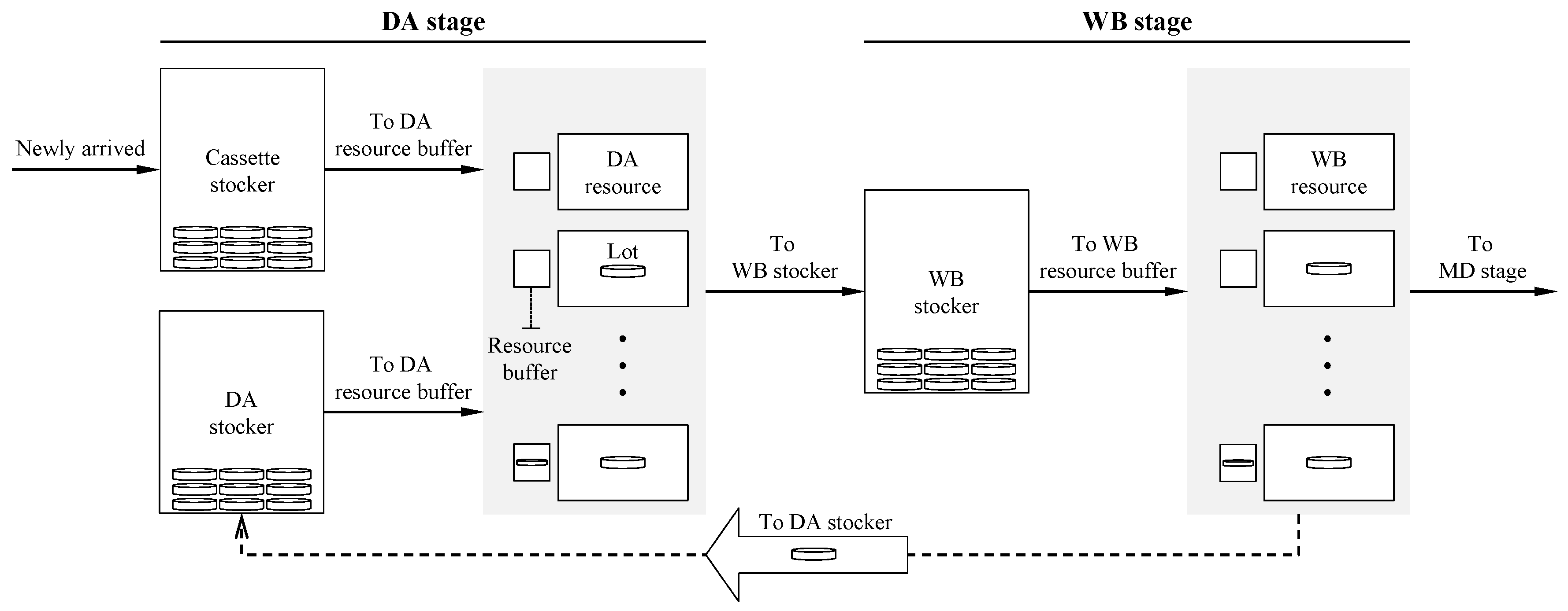
Figure 1 illustrates the lot flow of the MCP production process considered in this paper. Specifically, a lot is required to be processed in the DA stage prior to the WB stage, and the final operation of a lot is to complete in the WB stage. The dashed line at the bottom represents the flow of lots which revisit the DA stage after finishing the WB operation.

As shown in Figure 1, there are three types of stockers, namely cassette, DA, and WB stockers where lots stay temporarily. First, the cassette stocker provides locations for where newly arrived lots wait for the first DA operation. Next, the DA stocker is a place where lots that have completed a WB operation wait for the re-entrance to the next DA operation. Finally, the WB stocker is where lots that have completed a DA operation wait before they enter their WB operation.

Lots in either the cassette or DA stockers are transported to the WB stocker after DA operations are finished. This means that newly arrived and re-entrant lots are located together in the WB stocker, which yields complex lot flows. For this reason, it becomes challenging to manage the WIP level of the WB stocker at appropriate level, which is highly likely to decrease the utilization of the WB resources or increase the waiting time of lots in the WB stocker.

In front of each resource, there is a resource buffer in which a lot waits for the operation until the resource becomes idle. The capacity of a resource buffer is assumed to be one. A lot is not interrupted once its operation starts, and an operation is carried out by one resource at a time. Additionally, it is assumed that there is no setup time between lots of different job types.

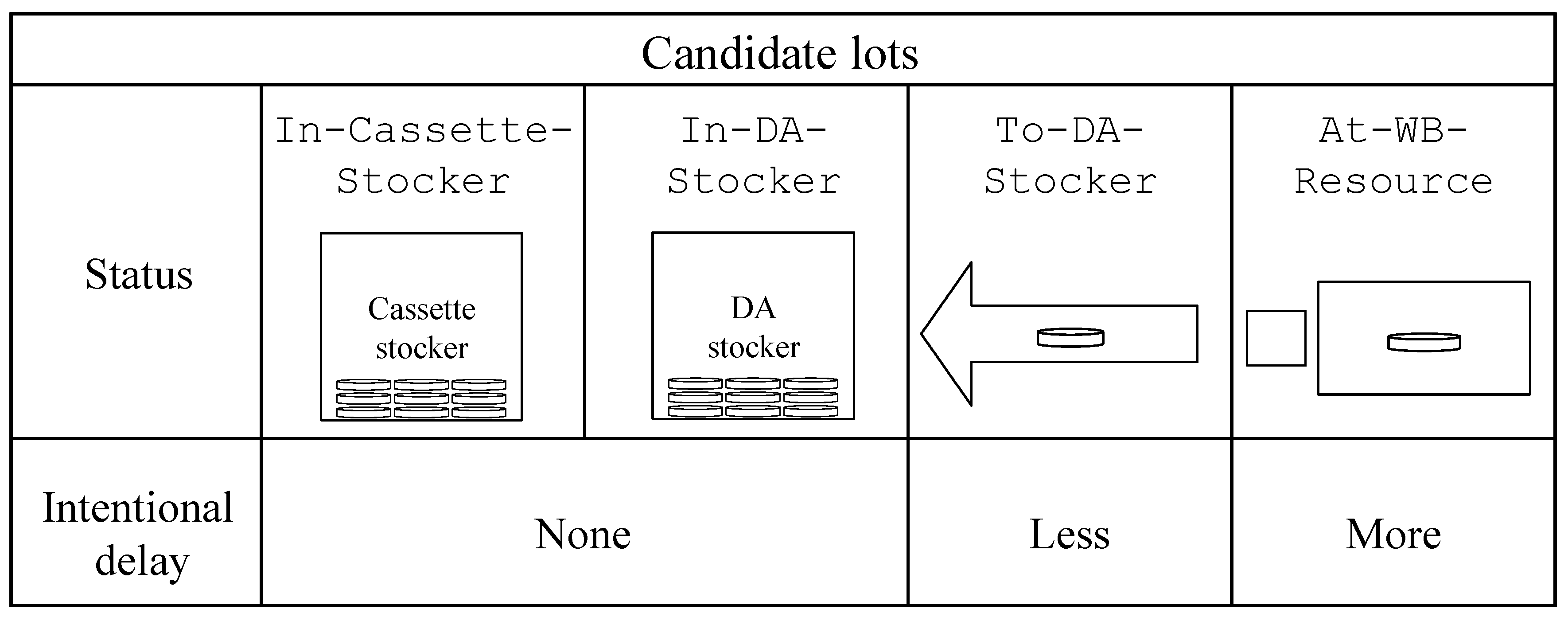
Furthermore, a candidate lot refers to one that is assignable to a DA resource when its resource buffer is empty. The types of a candidate lot according to its status are illustrated in Figure 2. A lot-dispatching method determines the assignment between a candidate lot, $L_{i,k}$, and a DA resource with an empty resource buffer, $R_{q,s}$, based on the decision policy if $M_q\in A\left(O_{i,I\left(L_{i,k}\right)}\right)$. Furthermore, once a lot is dispatched, it is excluded from the candidate lots.

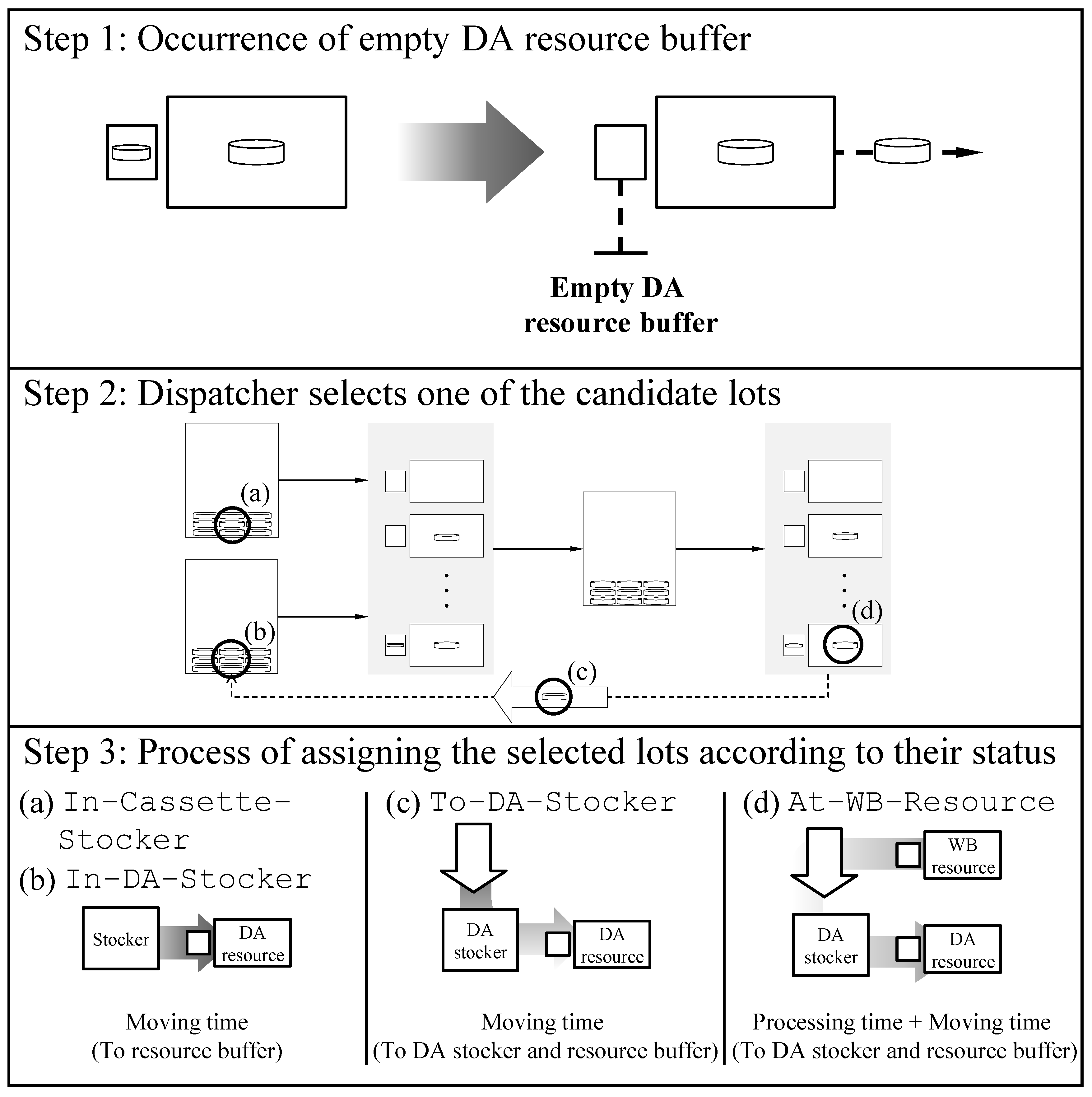
For a DA resource, a lot can be moved from the stocker to the DA resource buffer immediately whenever a candidate lot whose status is In-Cassette-Stocker or In-DA-Stocker is selected to be dispatched. In particular, the flow time of a lot begins to be measured when the lot in the cassette stocker is dispatched. Otherwise, in case that a candidate lot whose status is either To-DA-Stocker or At-WB-Resource is selected, this results in an intentional delay on the DA resource due to the additional time to carry out the remaining WB operation and/or to arrive at a DA stocker. The details of how the dispatcher assigns a lot to a DA resource are described in Figure 3. The bottom part of the step 3 shows the time for each lot to arrive the DA resource after the lot is selected by the dispatcher.

In the WB stage, intentional delays are not necessary since high utilization of resources should be achieved. Accordingly, among the lots in the WB stocker, the lot with longest processing time is assigned to a WB resource when its resource buffer is empty.

3. Proposed Framework

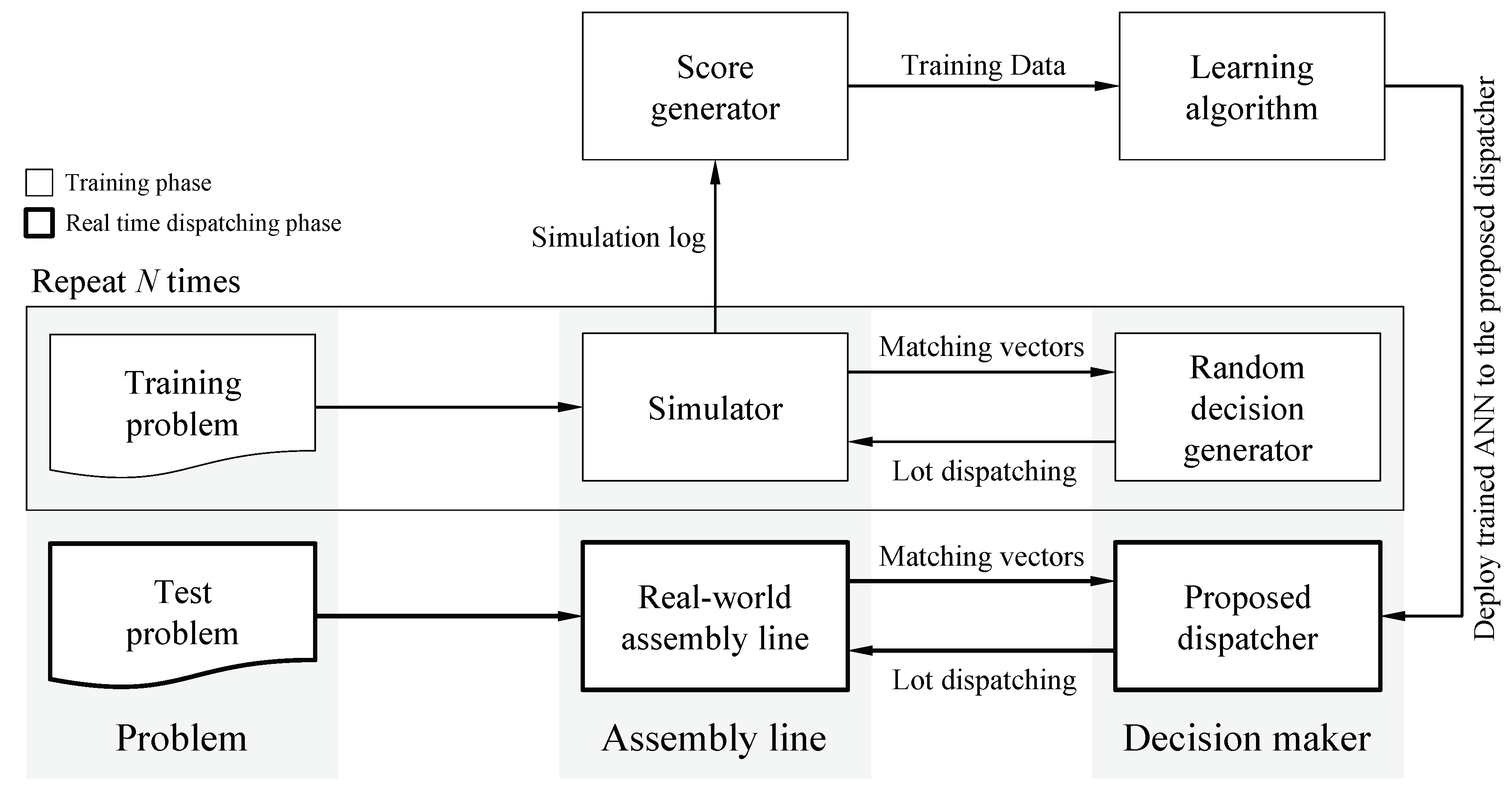
Figure 4 depicts the overall process of the proposed framework. In the training phase, we deploy a simulator that executes the DA and WB stages in MCP production as shown in Figure 1 to generate simulation logs. By using the simulator, all lot dispatching decisions of a problem are determined using a random decision generator (RDG) which is responsible for randomly assigning one of the candidate lots to a DA resource with empty buffer. The performances of the decisions by RDG are then measured, and the scored simulation logs will be used by a learning algorithm to train the ANN embedded in the proposed dispatcher. In the real-time dispatching phase, for a given test problem, the simulator calls the trained dispatcher whenever a lot dispatching decision is required.

3.1. Dispatcher Structure

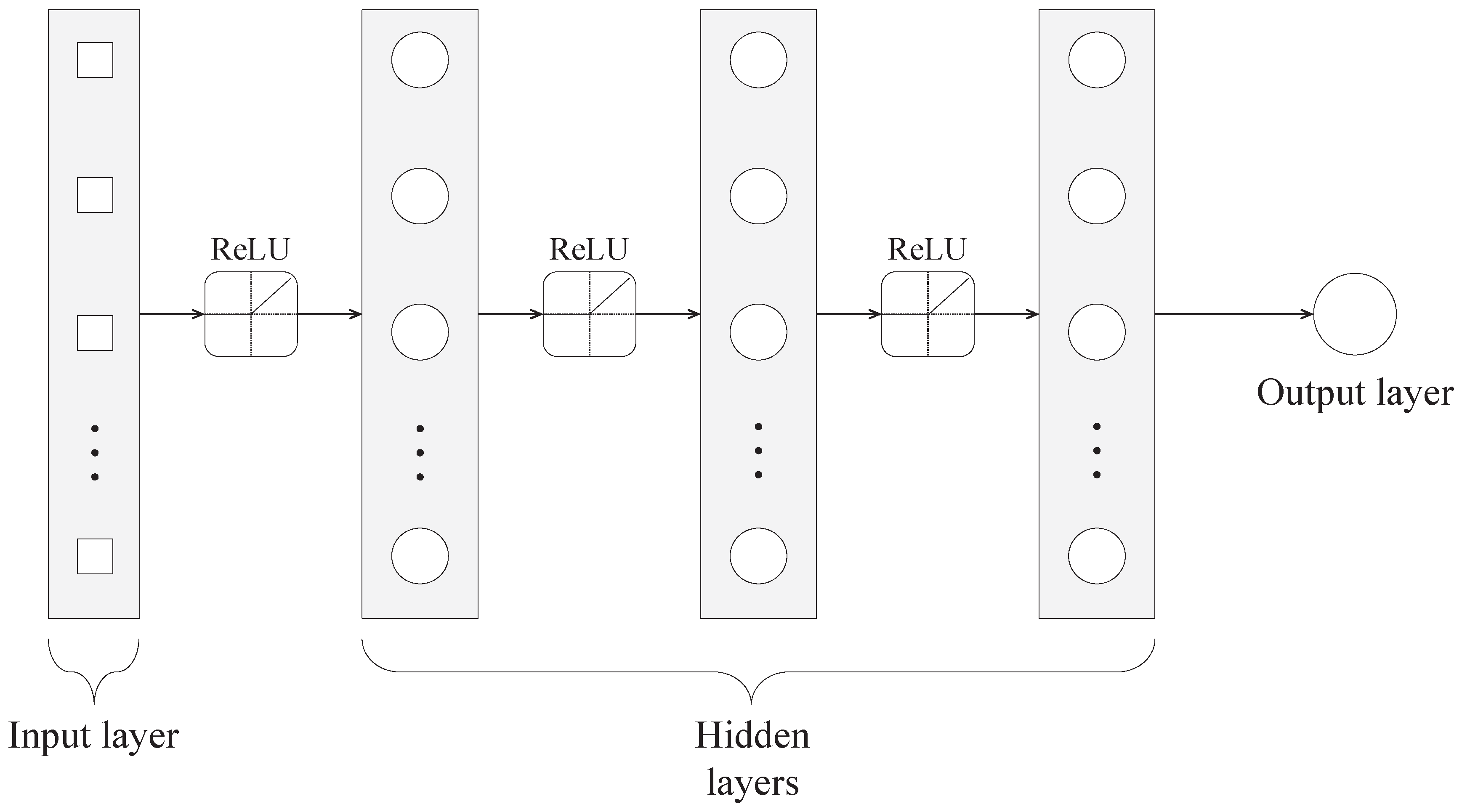
Figure 5 illustrates the architecture of the proposed dispatcher which consists of five layers: an input layer, three hidden layers, and an output layer. The input layer contains seven nodes, and the number of nodes in each hidden layer is set to seven, whereas the output layer has one node. The numbers of hidden layers and nodes in the hidden layers are empirically determined to reduce the training error. The rectified linear unit (ReLU) is applied before each hidden layer in order to provide a non-linear transformation, and all layers are fully connected [40].

A pair of a lots among the candidate lots and a DA resource is represented as a vector called a lot-DA assignment vector for the input to the proposed dispatcher. Specifically,

Table 2. Components of the lot-DA assignment vector, for $L_{i,k}$ and $R_{q,s}$.

Categories	Descriptions	Units
Conflicting lots of $L_{i,k}$	# of conflicting lots being moved from cassette and DA stockers to DA resource buffers	Quantity
	# of conflicting lots in DA resource buffers
	# of conflicting lots being processed on DA resources
	# of conflicting lots being moved from DA resources to a WB stocker
	# of conflicting lots waiting in the WB stocker
WB resource	# of WB resources that are able to process $L_{i,k}$	Quantity
Delay time	The interval between the time when the lot dispatching decision is made and the time when $L_{i,k}$ starts to be processed by $R_{q,s}$	Second

presents the components of the lot-DA assignment vector, for a particular lot, $L_{i,k}$, and a particular DA resource, $R_{q,s}$. Since the idle time of WB resources is one of the consisting term of the loss time considered, most features of the vector are defined based on the information related to the WB stage.

Using the defined features of a lot-DA assignment vector, the proposed dispatcher has the ability to predict how long the lot waits at the WB stocker after it is processed by a DA resource. Furthermore, the features provide a clue for estimating the idle time of the WB resource that will process the lot involved in the vector. As a result, the proposed dispatcher is expected to be able to conduct lot dispatching decisions which reduce the waiting time of lots and the idle time of WB resources.

Specifically, the lot-DA assignment vector contains seven features categorized into conflicting lots, available WB resources, and the delay time as follows. First, the concept of conflicting lots is introduced to represent lots that compete for WB resources. Lot, $L_{i^{\prime },k^{\prime }}$, is called a conflicting lot of $L_{i,k}$ if $L_{i^{\prime },k^{\prime }}$ and $L_{i,k}$ satisfy either one of the conditions presented in Equations (1) and (2).

$$A\left(O_{i^{\prime },I\left(L_{i^{\prime },k^{\prime }}\right)}\right)\cap A\left(O_{i,I\left(L_{i,k}\right)+1}\right)\ne \varnothing$$

(1)

$$A\left(O_{i^{\prime },I\left(L_{i^{\prime },k^{\prime }}\right)+1}\right)\cap A\left(O_{i,I\left(L_{i,k}\right)+1}\right)\ne \varnothing$$

(2)

The five features corresponding to the conflicting lots of $L_{i,k}$ are presented in Table 2 according to their status. Each feature represents the number of conflicting lots that correspond to one of the five different states. The proposed dispatcher can capture the distribution of the lots by collectively using all these features.

Next, the number of WB resources capable of processing a lot is included as a feature to capture the degree of potential conflict among the lots in the WB stage. In contrast to other features, this feature for a lot has a fixed value according to its resource type required in the WB stage regardless of the other lot dispatching decisions.

Finally, the delay time refers to how long it takes from the moment the lot dispatching decision is made until $R_{q,s}$ starts processing $L_{i,k}$. If the status of $L_{i,k}$ is In-Cassette-Stocker or In-DA-Stocker, the value of the delay time is calculated as the sum of the time required for $L_{i,k}$ to move from the stocker to the buffer of $R_{q,s}$ and the time that $L_{i,k}$ spends in the buffer. Otherwise, the time required for $L_{i,k}$ to move from the current location to DA stocker is added to the value mentioned above. Through this feature, the proposed dispatcher is capable of inferring whether or not $L_{i,k}$ causes an intentional delay in $R_{q,s}$.

The output layer represents the preference score of the assignment vector. All values in each node are normalized to a range [0, 1] using the min-max normalization to accommodate the inconsistencies of different units [41].

3.2. Training Phase

In the training phase, each generated problem is solved multiple times by using RDG. To obtain various simulation logs in terms of the flow time and resource utilization, for each simulation, the intentional delay level with a value between 0 and 1 is randomly selected. The intentional delay level close to one means a high probability of selecting lot whose status is To-DA-Stocker or At-WB-Resource, whereas the intentional delay level close to zero indicates a high probability of selecting lot whose status is in In-Cassette-Stocker or In-DA-Stocker.

Specifically, whenever a lot dispatching is required, a new random number with a value between 0 and 1 is generated. If this random number does not exceed the intentional delay level for that simulation, RDG makes a dispatching decision by using only lots whose statuses are To-DA-Stocker or At-WB-Resource among candidates, to simulate the intentional delay by letting the DA resource associated with the decision to be idle until the dispatched lot ready to be processed by the resource.

Once all lot dispatching decisions of each problem are determined by RDG, the generated simulation log containing the entire dispatching history each of which consists of a dispatched lot and an assigned DA resource, and their lot-DA assignment vector is sent to the score generator.

The score generator evaluates each lot dispatching decision based on the waiting time of the dispatched lot and the idle time of the WB resource that processed the lot. Here, the waiting time indicates the time during which a lot stays in the WB stocker after being completed by a DA resource. In contrast, the idle time of WB resource is calculated by subtracting the time at which its last operation ends from the time at which it starts processing the lot.

For each dispatching decision, the loss time defined above is denoted here as l. Based on l, the score generator calculates the score of a decision in the range of [0, 1] according to the concept of min-max normalization as presented in Equation (3) [41].

$$score=max(-(\frac{l-l_{min}}{l_{max}-l_{min}}(s_{max}-s_{min}))+s_{max},s_{min}),$$

(3)

where $l_{min}$ and $l_{max}$ respectively stand for the minimum and maximum values among all the possible values of l, and $s_{min}$ and $s_{max}$ refer to the minimum and maximum values among the possible values of score, respectively.

In Equation (3), $l_{max}$ is set to be twice the median of l values. This prevents a considerably high l from being converted to an unwanted positive score, which makes it possible to construct well-balanced training data. This is reasonable because we do not focus on predicting l precisely; the primary aim is to determine the lot dispatching decision expected to minimize l.

As a loss function, we used a squared error [42], defined as ${(score-scor{e}_{pre})}^2$, and the back-propagation training algorithm is used to minimize the loss function [43]. Here, $score$ is the calculated score value for a dispatching decision by using Equation (3) and $scor{e}_{pre}$ means the preference score for the decision in the training phase.

3.3. Real-Time Dispatching Phase

In the real-time dispatching phase, when a DA resource buffer is empty, lot-DA assignment vectors for all the possible assignments between candidate lots and DA resources are generated.

The generated lot-DA assignment vectors are given to the proposed dispatcher as the input, and the proposed dispatcher calculates the preference score of each vector. After this calculation, the lot and DA resource involved in the vector with the highest scores are selected as the lot dispatching decision. As a result, the lot is assigned to the DA resource.

The proposed dispatcher is anticipated to reach a better lot dispatching decision quickly compared to the conventional meta-heuristics through a simple calculation using the weights predetermined during the training. Therefore, it is expected that the proposed method can be introduced into the real-world assembly lines where lot dispatching decisions are required to be determined in a real-time manner.

4. Experiments

To show the effectiveness of the performances of the proposed dispatcher, we prepared three datasets by varying the composition of job types while fixing the total numbers of lots in each problem. A lot has several chips uniformly distributed between 74 and 370. Each dataset contains five job types with various numbers of lots. The characteristics of the datasets are summarized in

Table 3. Descriptions on the datasets used for the experiments.

Dataset No.	Avg. Number of Lots of Each Job Type					Avg. Number of Operations
	${\mathit{J}}_1$	${\mathit{J}}_2$	${\mathit{J}}_3$	${\mathit{J}}_4$	${\mathit{J}}_5$
1	34.50	24.66	24.06	24.46	14.46	526.08
2	24.31	24.48	24.43	24.84	24.72	590.97
3	14.25	24.71	24.13	24.37	34.36	644.87

.

The three datasets represent the different levels of difficulty for the dispatching problem of assembly lines. In this experiment, the difficulty is assessed in terms of the number of operations to complete the entire processing of lots. As the number of operations involved in a dataset increases, its computational complexity grows because the number of decisions required to resolve problems of the dataset increases proportionally.

Table 4. Problem description for experiments.

${\mathit{J}}_{\mathit{i}}$	${\mathit{O}}_{\mathit{i},\mathit{j}}$	Stages	$\mathit{A}\left({\mathit{O}}_{\mathit{i},\mathit{j}}\right)$	Processing Time
$J_1$	$O_{1,1}$	DA	($M_1$, $M_2$, $M_3$)	(1.4, 1.4, 2.1)
	$O_{1,2}$	WB	($M_4$, $M_5$, $M_6$)	(14.4, 16.2, 16.2)
$J_2$	$O_{2,1}$	DA	($M_1$, $M_2$, $M_3$)	(2.8, 3.5, 2.8)
	$O_{2,2}$	WB	($M_4$, $M_5$, $M_6$)	(23.4, 25.2, 25.2)
	$O_{2,3}$	DA	($M_1$, $M_2$, $M_3$)	(3.5, 3.5, 3.5)
	$O_{2,4}$	WB	($M_4$, $M_5$, $M_6$)	(23.4, 25.2, 25.2)
$J_3$	$O_{3,1}$	DA	($M_2$, $M_3$)	(3.5, 2.8)
	$O_{3,2}$	WB	($M_4$, $M_5$, $M_6$)	(32.4, 32.4, 36)
	$O_{3,3}$	DA	($M_2$, $M_3$)	(3.5, 3.5)
	$O_{3,4}$	WB	($M_4$, $M_5$, $M_6$)	(39.6, 41.4, 39.6)
$J_4$	$O_{4,1}$	DA	($M_2$, $M_3$)	(4.2, 4.2)
	$O_{4,2}$	WB	($M_4$, $M_5$, $M_6$)	(32.4, 32.4, 36)
	$O_{4,3}$	DA	($M_2$, $M_3$)	(3.5, 3.5)
	$O_{4,4}$	WB	($M_4$, $M_6$)	(36, 63)
	$O_{4,5}$	DA	($M_2$, $M_3$)	(3.5, 3.5)
	$O_{4,6}$	WB	($M_5$, $M_6$)	(41.4, 39.6)
$J_5$	$O_{5,1}$	DA	($M_1$, $M_2$, $M_3$)	(2.8, 2.8, 2.1)
	$O_{5,2}$	WB	($M_4$, $M_5$, $M_6$)	(50.4, 45, 45)
	$O_{5,3}$	DA	($M_1$, $M_2$)	(2.8, 2.8)
	$O_{5,4}$	WB	($M_4$, $M_5$, $M_6$)	(36, 36, 21.6)
	$O_{5,5}$	DA	($M_1$, $M_2$)	(2.1, 2.1)
	$O_{5,6}$	WB	($M_4$, $M_5$, $M_6$)	(36, 36, 21.6)
	$O_{5,7}$	DA	($M_1$, $M_2$, $M_3$)	(2.1, 2.1, 2.1)
	$O_{5,8}$	WB	($M_4$, $M_5$, $M_6$)	(36, 36, 21.6)

represents the operations of each job type and resource types that can perform each operation. The odd-numbered operations of a job type are assumed to be processed in the DA stage, whereas the even-numbered operations are processed in the WB stage. The last column in Table 4 shows the processing time of each operation per chip in the corresponding resource type. Additionally, the time required for a lot to move from the stocker to the resource buffer and vice versa is 900 s.

As shown in Table 4, the greater an index a job type has, the longer the number of operations that belong to the job type is. Compared to datasets 1 and 2, dataset 3 has problems where the number of lots of $J_5$ is greater than that of the other job types. Accordingly, dataset 3 has the greatest number of operations and high complexity among datasets.

For each dataset, 200 problems were generated by varying the quantity of the lots and the total number of lots for each job type. Specifically, 50 problems were used to train the proposed dispatcher, while the remaining problems were used to test the performance of the proposed dispatcher after it was trained. It is assumed that each dataset has several lots requiring more than two days for all lots to leave the assembly line, which is the well-known practice of the assembly line considered [2]. In the experiments, $N_M$ and $N_J$ are set to be 6 and 5, respectively. Specifically, for each problem, both the DA and WB stages have three different resource types, with 4 and 12 resources respectively assigned to them.

In the training phase, we generated simulation logs by solving each problem 500 times using RDG. The scores of the generated simulation logs were calculated by the score generator through using Equation (3). The performance of lot dispatching is measured by means of the waiting time of lots and the idle time of the resources of the WB stage. Specifically, the average waiting time of lots, $AWT$, is calculated as:

$$AWT=\frac{{\sum }_{i=1}^{N_J}{\sum }_{k=1}^{n_i}(c_{i,k}-r_{i,k}-t_{i,k})}{{\sum }_{i=1}^{N_J}{n}_i},$$

(4)

where $c_{i,k}$ and $r_{i,k}$ are the time that the last WB operation of $L_{i,k}$ is completed and $L_{i,k}$ leaves the cassette stocker, respectively, and $t_{i,k}$ indicates the sum of processing time of $L_{i,k}$ on resources.

Additionally, the average idle time of the WB resources, $AIT$, is defined as follows:

$$AIT=\frac{{\displaystyle \sum _{\forall q\in \mathsf{\Omega }}}{\displaystyle \sum _{s=1}^{n_q}}(f_{q,s}-t_{q,s})}{{\displaystyle \sum _{\forall q\in \mathsf{\Omega }}}{n}_q},$$

(5)

where $f_{q,s}$ represents the time at which $R_{q,s}$ completes its last operation and $t_{q,s}$ is the total processing time of the operations assigned to $R_{q,s}$ between time 0 and $f_{q,s}$, and $\mathsf{\Omega }$ is a set of indexes of the resource types which belong to the WB stage. Moreover, to collectively measure the overall performance in terms of $AWT$ and $AIT$, we used the average loss time denoted as $ALT$ that is the sum of these two values.

After we trained three instances of the proposed dispatcher for each dataset, the dispatcher generated by the training data of dataset 3 outperformed the others under all the datasets. Therefore, we used this instance of the dispatcher for all the experiments performed in this research.

For the comparison purposes, we implemented the conventional dispatching rules such as the first-in-first-out (FIFO), the last-in-first-out (LIFO), the most-operations-remaining (MOR), and the least-operations-remaining (LOR), all of which are widely used to reduce the flow time or increase resources utilization [44]. In particular, LIFO is known to perform better in terms of minimizing the maximum and mean flow time in dynamic job shop scheduling problem [45]. Here, FIFO selects the oldest lot that has been dispatched from the cassette stocker among the candidate lots, while LIFO addresses the latest one that has been dispatched. Both rules randomly dispatch the lot from the cassette stocker when the lots whose status is In-Cassette-Stocker exist in the candidate lots only.

Furthermore, we also compared the proposed dispatcher with the composite dispatching rule using SVR proposed by [27]. The dispatching rules mentioned above are used to construct a linear combination of the composite dispatching rule. The weight assigned to each rule is determined by the model trained with SVR whenever a lot dispatching decision is required. The feature set and the parameters of SVR used in the experiments are identical to those in [27].

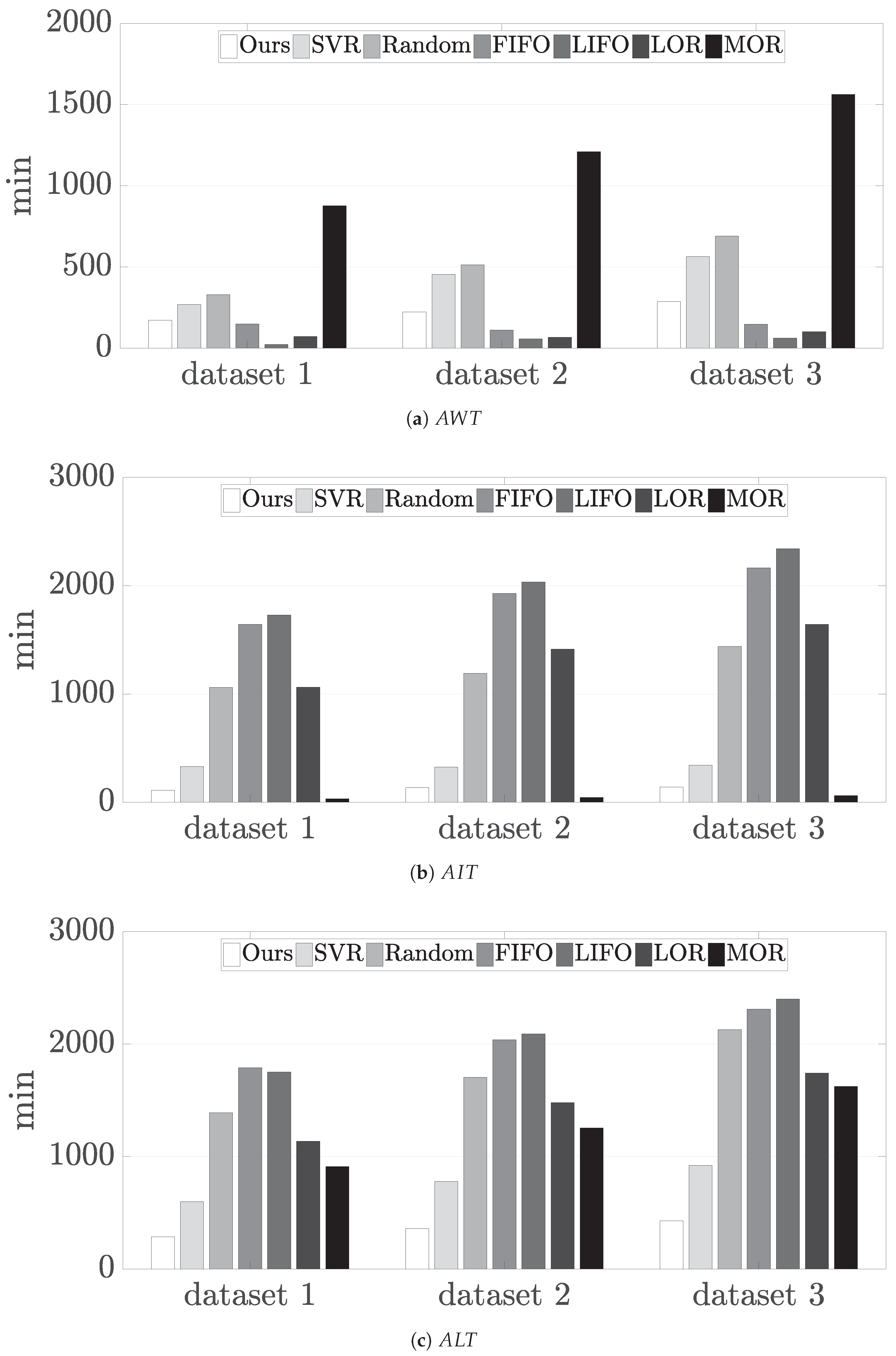
The performance comparison results for the proposed dispatcher, RDG, and the other dispatching methods considered under each dataset are presented in Figure 6, where Figure 6a–c show the results for $AWT$, $AIT$, and $ALT$, respectively. In terms of $AWT$, FIFO, LIFO, and LOR shows the better performances than the proposed dispatcher for all the datasets. This is because FIFO and LIFO assign a low priority level to the lot whose status is In-Cassette-Stocker, and LOR prefers the job type whose number of operation is small. As a result, the waiting time of lots are reduced owing to the decrease in the number of lots in the WB stocker. However, these simple policy causes an increase in the probability that the WB resources become idle eventually. As shown in Figure 6b, these rules lead to made excessively large value of $AIT$.

MOR tends to disallow resources from being idle since this rule assigns a high priority level to lots according to the number of operations to be processed. Although this might result in almost zero $AIT$, it yields a considerable $AWT$ compared to all the other methods including the proposed dispatcher due to the increased WIP level.

Meanwhile, in terms of $ALT$, the proposed dispatcher and SVR outperformed the other methods in all datasets, as shown in Figure 6c. However, SVR showed lower performances than the proposed dispatcher in terms of all performance measures. This is due to the lack of features that can represent the concept of conflicting lots and predict intentional delay even though SVR attempts to choose the proper dispatching rule according to a given assembly line state. In addition, the performance difference between two methods can be attributed to the fact that the proposed method is possible to select one of candidate lots while SVR performs one of the existing dispatching rules.

Table 5. $ALT$ improvement rate of the proposed dispatcher compared to existing methods.

Dataset No.	SVR	RDG	FIFO	LIFO	LOR	MOR
1	53%	80%	85%	84%	75%	69%
2	55%	79%	83%	83%	76%	72%
3	54%	80%	82%	83%	76%	74%

highlights the improvement rate of the proposed dispatcher over the other dispatching methods in terms of $ALT$. The proposed dispatcher has reduced $ALT$ from at least 53% to 85% compared to the existing methods. Furthermore, as shown in

Table 6. Significant difference in $ALT$ between the proposed dispatcher and existing methods.

Dataset No.	SVR	RDG	FIFO	LIFO	LOR	MOR
1	313.25	1105.75	1505.36	1466.09	851.14	625.32
	6.99 × 10−81	3.22 × 10−51	1.01 × 10−127	3.38 × 10−130	3.15 × 10−102	2.33 × 10−121
2	420.76	1345.44	1679.17	1731.36	1121.52	895.17
	5.99 × 10−72	5.79 × 10−51	4.99 × 10−49	1.70 × 10−73	6.26 × 10−71	5.72 × 10−115
3	491.54	1698.65	1883.17	1972.73	1313.5	1195.98
	7.38 × 10−94	7.46 × 10−56	9.48 × 10−142	6.34 × 10−151	1.46 × 10−140	2.87 × 10−104

, the statistically significant differences in $ALT$ between the proposed dispatcher and the existing methods are investigated by the t-test at the 1% level presented. The top number in each cell means the difference in $ALT$ between the proposed dispatcher and the existing method corresponding to each column, and the bottom number indicates the corresponding p-value. All p-values in Table 6 are less than 0.01, which confirms the results of Figure 6c and Table 5.

Based on the above observation, the proposed dispatcher successfully reduces both $AWT$ and $AIT$ at the same time in contrast to the existing methods which focus only on one performance measure. Therefore, the proposed dispatcher appears to achieve a reduction in the flow time while maintaining high utilization of resources in the bottleneck stage.

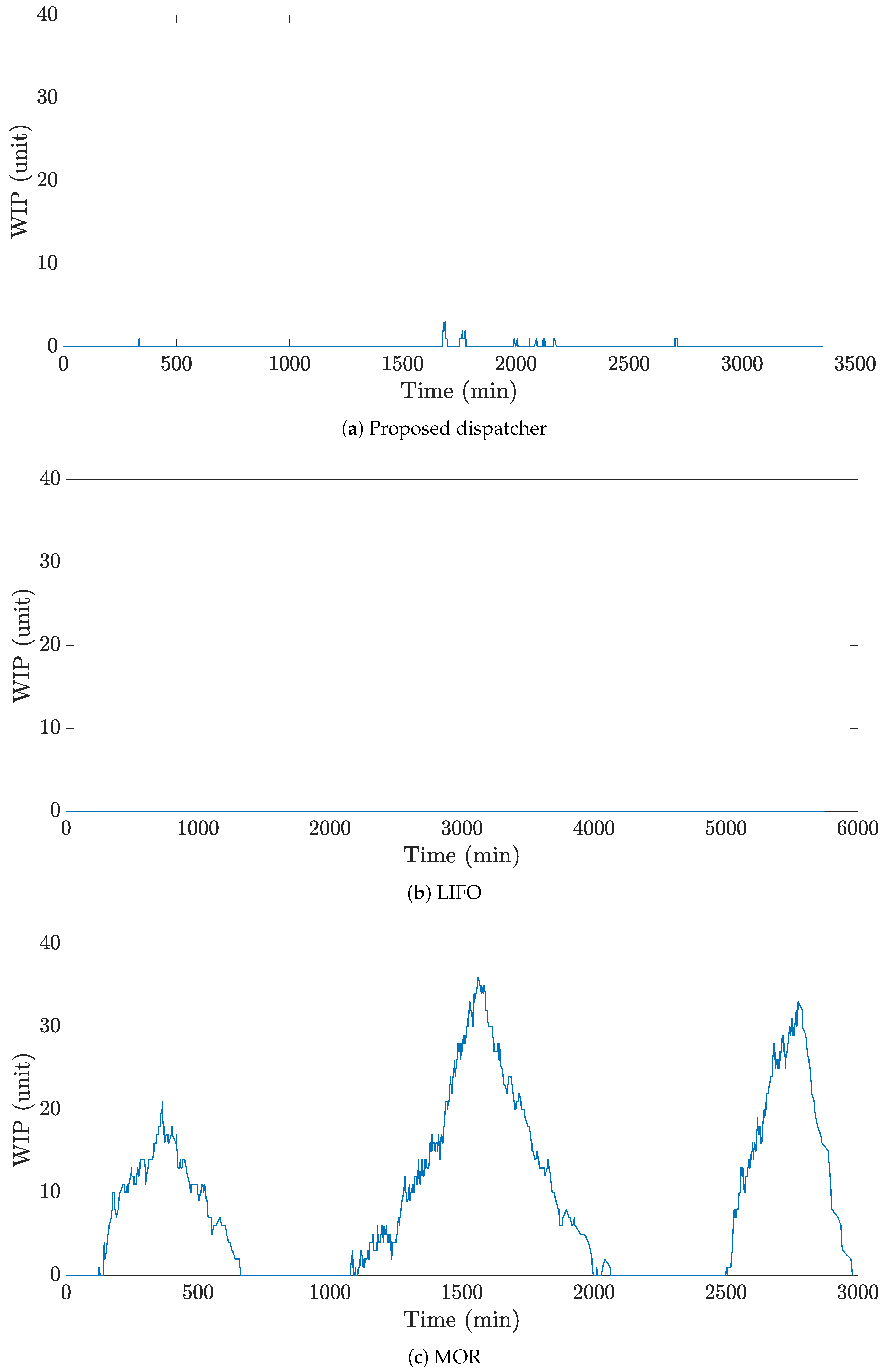
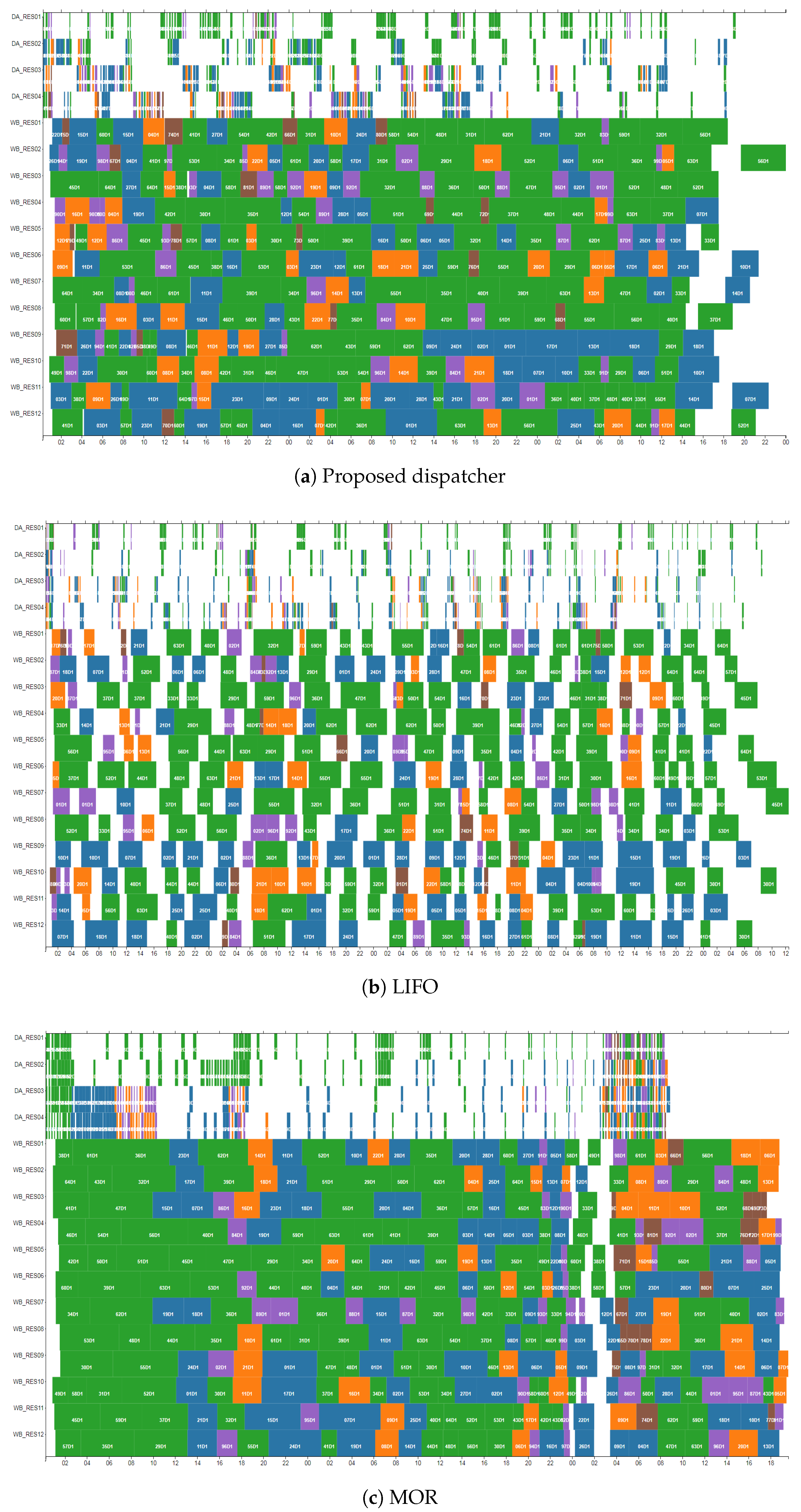
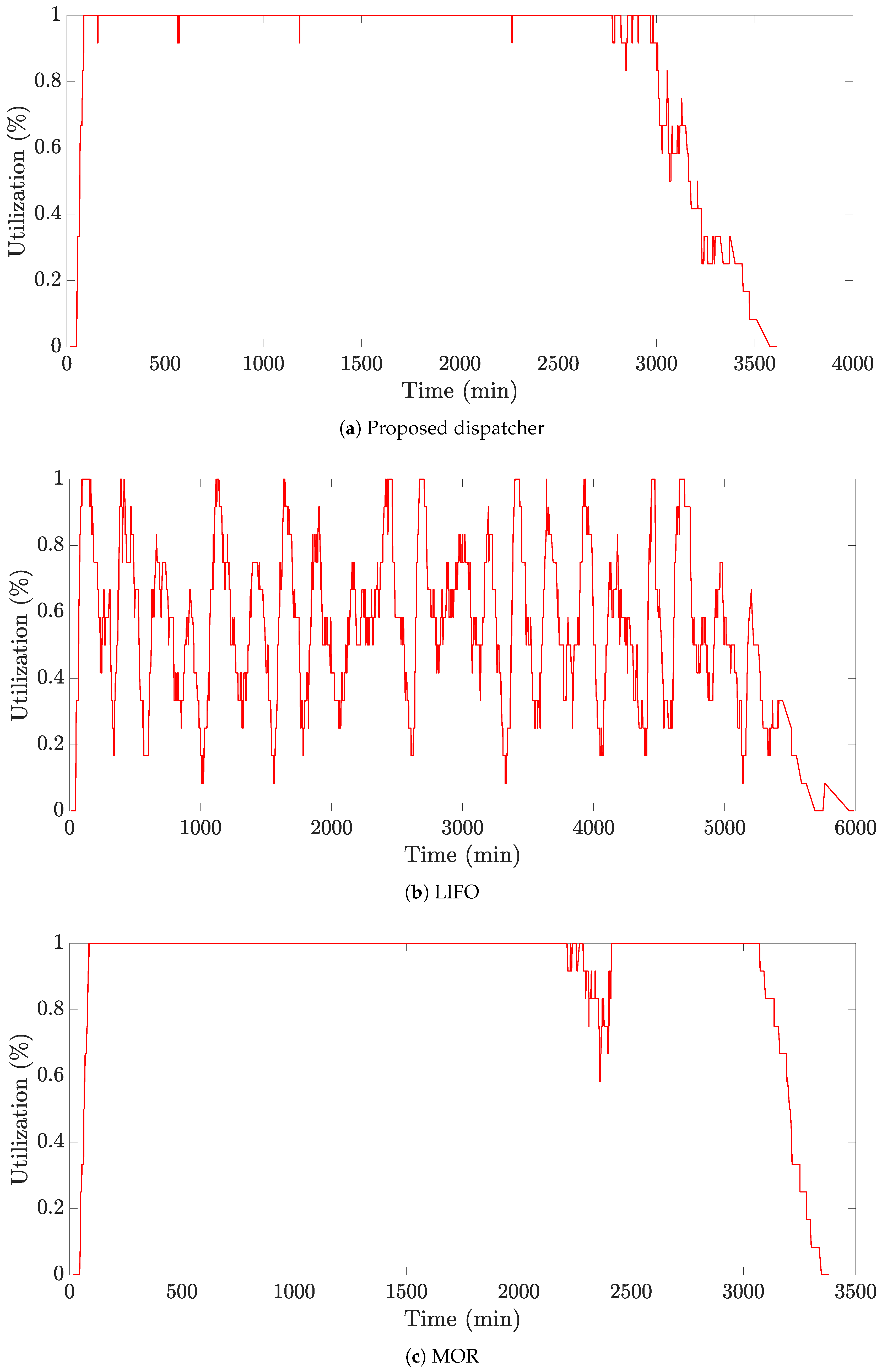
We provide a further analysis of the effects of lot dispatching decisions. Figure 7, Figure 8 and Figure 9 present the dispatching results of each resource over time, an utilization of the WB resources, and the WIP level of the WB stocker obtained by using dataset 3, respectively. Here, the values in the utilization graph represent the number of WB resources processing a lot divided by the total number of WB resources.

According to Figure 7a, the proposed dispatcher keeps the WIP level close to zero while always maintaining the utilization rate of WB resources at approximately 100% at all times (shown in Figure 8a and Figure 9a). These successful performances might be attributed to the sophisticated dispatching ability of the proposed dispatcher than the existing dispatching rules.

In contrast to the proposed dispatcher, as presented in Figure 7b, LIFO reduces the waiting time by maintaining an extremely low WIP level. However, this causes WB resources to be idle frequently, resulting in the severe fluctuations of the utilization for the WB resources (shown in Figure 8b and Figure 9b).

Figure 8c and Figure 9c indicate that MOR continues to run WB resources by keeping the WIP at a high level, leading to inevitable increases in the waiting time. However, it was observed that the WIP level drops to 0 between 750 and 1000 min and between 2000 and 2500 min (shown in Figure 7c). This arises due to the fact that MOR prevents the selection of lots with few remaining operations in the cassette stocker.

Additionally, we compared the lot dispatching decision patterns over time by the proposed dispatcher, LIFO, and MOR. In Figure 10, heat maps visualize the frequency of status of the lots dispatched by each dispatching method over time, where Figure 10a–c represent the results of the proposed dispatcher, LIFO, and MOR, respectively. The value in Figure 10 indicates the number of dispatched lots that correspond to each status for the interval of three hours.

In Figure 10a, the proposed dispatcher appears to increase the utilization of WB resources by dispatching the lots whose status is In-Cassette-Stocker at an early stage with a low WIP level. Subsequently, when the WIP level reaches a sufficient level, it tends to prevent the waiting time of lots from increasing by dispatching the lots whose status is In-DA-Stocker or At-WB-Resource.

On the other hand, Figure 10b indicates that LIFO assigns a higher priority to the lots whose status is At-WB-Resource. As a result, the time required to complete the dispatching of all lots becomes longer compared to those in the other methods. In contrast to LIFO, the results illustrated in Figure 10c present that MOR shows a tendency to concentrate on the dispatching lots whose status is In-Cassette-Stocker, which increases the waiting time of lots due to the rise in the WIP level, although this behavior enables to keep the utilization of WB resources high.

Finally, an analysis of the effects of the intentional delay decision was conducted.

Table 7. $ALT$ improvement rates achieved by allowing intentional delays.

Dataset No.	Ours	SVR	RDG	FIFO	LIFO	LOR	MOR
1	63%	6%	−81%	−141%	−133%	−86%	−12%
2	63%	6%	−79%	−121%	−130%	−94%	−26%
3	61%	8%	−95%	−121%	−133%	−90%	−44%

presents how much $ALT$ is reduced under the condition where intentional delays are allowed compared to when they are not. The negative values in the table indicates an increase in $ALT$ when intentional delays are allowed.

The result shows that the proposed dispatcher yielded better results when intentional delays were allowed. The solution space with intentional delays becomes wider than the other case because the lots whose status is To-DA-Stocker or At-WB-Resource are not included as candidate lots without intentional delays. Due to the advantage of ANN, which can capture complex patterns of data, the proposed dispatcher appears to obtain a superior solution in a widened solution space.

The existing dispatching methods except for SVR yielded significantly high values of $ALT$ with intentional delays. The rules which mainly focus to reduce the waiting time of lots, including FIFO, LIFO, and LOR, seem to be possible to shorten the idle time by eliminating intentional delays. Moreover, the decreased number of candidate lots alleviated the tendency of MOR to keep numerous lots in the DA stocker for a long time, leading to the decreased $AWT$. Although SVR succeeded in reducing $ALT$ when intentional delays were allowed, the improvement rates were much smaller than the proposed dispatcher for all datasets.

5. Conclusions

In this paper, we presented a novel method for reducing the waiting time of lots and the idle time of resources in the bottleneck stage of semiconductor MCP assembly lines by considering intentional delays. To learn an efficient lot dispatching policy at the DA stage with intentional delays, we employed ANN which has the ability to capture complex non-linear dynamics. Furthermore, the score generator was also proposed to obtain the training data for ANN by evaluating the performances of the decisions in randomly generated simulation logs.

The experiments demonstrate that the proposed method is successful in decreasing the flow time and increasing the utilization of bottleneck resources at the same time. In other words, the proposed method guarantees sustainability in terms of low WIP level and high resource utilization at the bottleneck stage. Specifically, the proposed dispatcher outperforms the traditional dispatching rules in terms of the loss time for all the datasets considered. Furthermore, through the comparison experiments without intentional delays, the proposed dispatcher yields better dispatching decisions than the existing methods especially when the problem becomes complex.

Although satisfactory results were obtained, there exist some other aspects needed to be considered to further improve the proposed method such as setup changes. Since setup change constraints are not only related to resource utilization but also to satisfying the production requirements, these are necessary to be taken into account from a global perspective. Therefore, we plan to investigate a reinforcement learning algorithm which is capable of finding a policy that maximizes global rewards in order to enable more intelligent dispatching under assembly lines with the setup change constraints.