A Multi-Objective Framework for Cost and Carbon-Optimal Vehicle Electrification Under Grid Constraints

Abstract

Electrification of road transport is widely promoted as a pathway to reduce greenhouse gas (GHG) emissions; however, its effectiveness depends critically on electricity carbon intensity, renewable energy share, charging behavior, and grid capacity constraints. This study develops a multi-objective analytical and optimization framework to evaluate cost and carbon-optimal electric vehicles electrification by jointly minimizing system cost and carbon emissions under coupled transport–energy system conditions. A closed form cut-off condition is derived to determine the minimum renewable electricity share required for electric vehicles to achieve lower emissions than internal combustion engine vehicles, and the formulation is extended to mixed fleets including battery electric and plug-in hybrid electric vehicles. The framework integrates fleet-level emissions, electricity demand, renewable capacity limits, charging losses, carbon taxation, and peak charging constraints to define a feasible electrification region. Feasibility mapping, Monte Carlo exploration, and evolutionary multi-objective optimization are employed to characterize trade-offs between CO₂ emission and total system cost, and to identify Pareto-optimal and knee point solutions. The results show that electrification without sufficient renewable support or coordinated charging can increase emissions and violate grid limits, whereas integrated planning enables significant emission reduction within economically viable regions. These findings provide a quantitative and decision-oriented basis for cut-off-informed and grid-aware electrification planning in carbon-constrained power systems.

1. Introduction

The transport sector is a major contributor to global greenhouse gas (GHG) emissions, largely driven by the widespread use of internal combustion engine vehicles (ICEVs) powered by fossil fuel. Passenger and commercial road transport account for a substantial share of energy-related carbon dioxide (CO₂) emissions worldwide, motivating governments to introduce regulatory, fiscal, and technological measures aimed at decarbonization [1,2]. Amongst these measures, the electrification of road transport has emerged as a key strategy to reduce tailpipe emissions and improve energy efficiency [3,4].

However, the environmental benefits of electric vehicles (EVs) are not unconditional. Several studies have shown that the net CO₂ reduction for EV adoption strongly depends on the carbon intensity of the electricity generation mix used for charging [5,6]. In regions where electricity is predominantly generated from coal or other carbon-intensive sources, EV charging may shift emissions from the transport sector to the power sector, potentially offsetting or even negating the expected climate benefits [5,7]. This coupling between transport electrification and power systems emissions necessitates an integrated assessment framework that jointly considers vehicle energy consumption, grid carbon intensity, and renewable energy penetration. In this study, the emission assessment is primarily focused on operational and electricity generation-related emissions relevant to transport–energy system planning. Full lifecycle emissions associated with vehicle manufacturing, battery production, recycling, and infrastructure construction are considered outside the immediate scope of the proposed analytical framework.

In addition to grid emissions, real-world vehicle operation characteristics play a critical role in determining the transport sector CO₂ emissions. Factors such as fuel type, driving behavior, vehicle efficiency and idling time significantly influence fuel consumption and emission rate for ICEVs [8,9]. Idling-related emissions, in particular, represent a non-negligible source of avoidable CO₂ emissions in urban environments and are often underestimated in high-level assessments [10,11]. Accurate representation of these effects is essential for fair comparison between ICEVs and EVs.

From a policy perspective, carbon pricing mechanisms such as carbon taxes and emission trading schemes are increasingly used to internalize the environmental cost of CO₂ emissions and incentivize low-carbon technology [12,13]. In countries such as South Africa, carbon taxation has been formally introduced for both transport fuel and electricity generation, directly affecting economies’ competitiveness of EVs relative to conventional vehicles [14]. Consequently, the optimal level of transport electrification must be evaluated not only from an emission standpoint but also from an integrated cost–carbon perspective.

Large-scale EV adoption also introduces new challenges for power system planning and operation. Uncoordinated EV charging can significantly increase the peak demand, stress, and energy distribution networks, and requires costly grid reinforcement [5,15]. Several studies have highlighted the importance of smart charging strategies, renewable powered charging infrastructure, and coordinated planning to mitigate these impacts while maximizing the emission reduction [16,17]. Nevertheless, a clear analytical link between maximum admissible EV penetration, renewable energy availability, and grid peak constraints remains insufficiently addressed in the literature.

Most existing studies focus either on lifecycle emission analysis [18], scenario-based projection [19] or system-level optimization in the power sector [15,20]. While valuable, these often adopt a transparent and analytically interpretable criterion that define when EV electrification becomes environmentally beneficial and how far electrification can be achieved under emission, cost and grid constraints. In particular, the concept of a cut-off condition defining the minimum renewable share or maximum electrification level beyond which EV deployment yields net CO₂ benefits has not been systematically formulated as a unified framework.

It is in this context that this study proposes a comprehensive analytical computational framework for evaluating the environmental, economic, and grid impacts of EV integration. The proposed framework is intended not only to optimize electrification pathways, but also to provide analytically interpretable feasibility boundaries capable of supporting transparent and scalable transport–energy planning under coupled operational constraints.

The main contributions of the paper are as follows:

• Analytical Cut-off Condition: A closed form condition is derived to determine the minimum renewable electricity share required for EV operation to outperform ICEVs in terms of CO₂ emissions, explicitly accounting for grid carbon intensity, vehicle energy consumption, and idling related emissions.
• Fleet-Level Emission Modeling: The proposed framework integrates ICEVs, BEVs, and plug-in hybrid electric vehicles (PHEVs) into a unified fleet emission model, enabling assessment of mixed technology transition pathways.
• Peak Load Constrained Electrification Analysis: A charging window-based peak demand model is introduced to quantify the maximum EV charging power requirement, and the corresponding maximum admissible electrification share under grid capacity limits.
• Cost–Carbon Multi-Objective Optimization: A combined emission cost optimization is performed using Monte Carlo sampling and evolutionary multi-objective optimization techniques, yielding Pareto front, knee point, and policy-relevant operating points.
• Policy Relevance: The proposed framework explicitly incorporates carbon taxation, and renewable energy limits, and grid constraints, providing actionable insights for policymakers and planners in emerging and carbon-intensive power systems.

Thus, by combining analytical clarity with detailed numerical analysis, this study provides a decision support tool for determining how much, how fast and under what condition EV electrification should be persued to achieve meaningful and cost-effective emission reductions.

The rest of the paper is organized as follows. Section 2 presents a comprehensive literature review on vehicle emission, EV integration and carbon mitigation policies. It highlights the limitations of current approaches in capturing grid dependency and system-level constraints. Section 3 presents the materials and methods systematically through four subsections. Firstly, it introduces the proposed analytical framework, including the formulation of emission models for ICEVs, EVs and PHEVs, and derives the electrification cut-off condition. Secondly, it extends the model to fleet-level analysis and incorporates the renewable energy allocation, carbon taxation, and cost structures. Thirdly, it presents the optimization methodology including multi-objective formulation, Pareto front construction, and the knee point identification. Finally, it introduces the grid-constrained peak charging modeling and derives the electrification limits under network capacity constraints. Section 4 presents the numerical case studies and scenarios analysis to illustrate the environmental, economic, and infrastructural trade-off of EV deployment under varying grid and policy conditions. It also discusses the policy implications such as how the results can be implemented for energy and transport planning. Section 5 concludes the paper by summarizing key findings, addressing limitations and outlining directions for future research.

2. Literature Review

This section presents a comprehensive literature review on vehicle emissions, EV integration and carbon mitigation policies, highlighting the limitations of current approaches in capturing grid dependency and system-level constraints. The section is divided systematically into several subsections, each dealing with a specific aspect of the reviewed literature.

2.1. Transport Emissions and Internal Combustion Vehicles

Road transport has been identified as a major contributor to CO₂ emissions due to fuel combustion in ICEVs. Mickūnaitis et al. [21] investigated fuel consumption reduction strategies and highlighted the sensitivity of emissions to driving conditions. Fontaras et al. [8] demonstrated that significant discrepancies exist between laboratory-certified fuel consumption values and real-world emissions, particularly under dynamic driving conditions.

Prati et al. [11] analyzed the impact of idling and stop–start conditions in urban environments, showing that such operating modes substantially increase fuel consumption and CO₂ emissions. Similarly, Das et al. [9] presented emission factors for estimates based on real-world vehicle data, confirming that traffic conditions, vehicle loading and driver behavior significantly influence emission levels.

Idling emission presents an important but often underestimated component of the transport sector CO₂ emissions. The US Department of Energy report [10] quantified idle fuel consumption rates for different vehicles by type, highlighting that significant fuel is consumed even when vehicles are stationary. Aries [22] further examined real-world idling behavior and demonstrated that prolonged idling in urban environments leads to substantial and avoidable fuel losses in terms of modeling. Agar et al. [23] incorporated GPS-based data to estimate emissions more accurately, demonstrating that including idling improves the reliability of emission calculations. Similarly, Ditl and Šulc [24] developed methodologies for CO₂ emission estimation from fuel use, establishing the importance of capturing non-driving energy consumption, including idling. The commercial fleet database [25] further supports this by offering practical emission calculation tolls that account for real-world operating conditions, including idle time.

The aforesaid studies collectively indicate that variations in driving cycle, traffic congestion, vehicles loading, and driver behavior are not adequately captured in standardized laboratory testing procedures. As a result, real-world emissions are often considerably higher than regulatory estimates, highlighting a key limitation in conventional emission assessment approaches. In the study [26], Hao further confirms that real-world emission variability is strongly influenced by dynamic driving patterns and operational uncertainties. In addition, these studies demonstrate that neglecting idling leads to systematic underestimation of transport emissions. Therefore, emission assessment frameworks must explicitly incorporate idling and low-speed operation to ensure accurate comparison between ICEVs and electric vehicle alternatives. This highlights the necessity of incorporating high-resolution operational data into emission modeling frameworks for improved accuracy [27].

2.2. Electric Vehicles and Grid Carbon Intensity

EVs are widely promoted as a low-emission alternative to ICEVs, primarily due to their zero tailpipe emissions and higher drivetrain efficiency. However, their overall climate benefit depends critically on the carbon intensity of the electricity used for charging. Naseem et al. in [28] emphasize that this dependency introduces significant regional variability in EV environmental performance. Schill and Gerbaulet [5] analyzed the interaction between EV charging and power generation mix, demonstrating that EVs charged in coal-dominated systems could lead to higher indirect emissions as compared to conventional vehicles. Yang and Wu [19] examined energy consumption and emission scenarios under different propulsion systems, showing that EV-related emissions vary significantly depending on regional electricity mixes. Solanki et al. [29] highlighted the role of distributed generation in reducing emissions, emphasizing that cleaner electricity supply directly improves the environmental performance of e-transport. Similarly, Mouli et al. [6] demonstrated that integrating renewable energy into EV charging infrastructures can significantly reduce both emissions and operational costs.

In carbon-intensive power systems, the environmental advantages of EVs can be diminished or even reversed. Chen et al. [30] showed that this effect becomes more pronounced under high charging demand scenarios without coordinated energy management. Kumari and Bera [7] investigated emission reduction strategies in coal-based power systems and showed that high grid carbon intensity can offset the benefits of electrification. Paraschiv and Paraschiv [1] analyzed long-term trends in fossil fuel emissions, reinforcing that regions heavily reliant on carbon-intensive generation face greater challenges in achieving net emission reduction through electrification.

Conversely, Costa and Seixas [31] demonstrated that EV deployment can substantially reduce urban emissions when supported by cleaner electricity supply. Gajanayake et al. [3] analyzed national-level scenarios and showed that increasing renewable penetration significantly enhances the environmental performance of EVs. Lajunen [4] further confirmed that EV emissions decrease as renewable energy share ($r$) increases, particularly under low-carbon electricity systems. Regional assessments across Europe, Asia and Latin America confirm that the environmental benefits of EVs are highly dependent on the location. Yang and Wu [19] illustrated regional variability in emission outcomes, while Gajanayake et al. [3] and Mouli et al. [6] emphasized that the effectiveness of EV adoption is closely tied to power system decarbonization pathways. Furthermore, Su and Chow [32] identified coupling EV charging with renewable generation as a key factor in maximizing emission reduction benefits.

Recent advances in battery analytics and charging optimization have further demonstrated the importance of incorporating charging-condition variability into EV performance assessment. Jia et al. [33] proposed a physics-informed ensemble learning framework for battery aging prediction under diverse charging conditions, integrating electro-thermal constraints with data-driven models to improve prediction accuracy and robustness across varying temperatures, charging protocols, and cut-off voltages [33]. Their findings highlight the importance of physically consistent charging models in improving EV operational reliability and sustainability assessments.

These findings collectively demonstrate that EV electrification does not inherently guarantee emission reduction. Instead, the environmental performance of EVs is strongly dependent on electricity generation characteristics, motivating the need for explicit analytical criteria linking EV deployment to renewable energy availability and grid carbon intensity.

2.3. Policy Instruments and Carbon Pricing

Carbon pricing mechanisms, including the carbon taxes and emissions trading systems, play a vital role in shaping transport and electricity sector decarbonization strategies. The 2017 Carbon Tax Guide [12] provides a comprehensive overview of carbon tax frameworks, demonstrating the effectiveness in internalizing the social cost of CO₂ emission and incentivizing low-carbon technologies. The Carbon Tax Discussion Paper [34] analyzed carbon tax policy design in the South African context, highlighting its role in influencing both fuel and electricity pricing structures. The Explanatory Memorandum on the Carbon Tax Bill by South African National Treasury [2] further formalized the implementation of carbon taxation, emphasizing its impact on emission reduction strategies across multiples sectors. In particular, the environmental levy framework for CO₂ emissions by the South African Revenue Service [14] shows that carbon taxation in South Africa applies to both transport fuel and electricity generation, directly affecting the comparative economic performance of ICEVs relative to electrified alternatives.

In the power sector, Olsen et al. [13] developed optimal carbon tax models to achieve emission reduction targets while minimizing system costs, demonstrating the importance of economically efficient policy design. Pereira et al. [35] examined the impact of flexible carbon tax schemes on power system expansion planning, showing that adaptive pricing mechanisms can significantly influence investment decisions. Similarly, Zhang et al. [36] incorporated carbon emission trading into unit commitment models, highlighting how market-based mechanisms affect operational planning decisions in electricity systems. Hoekstra [37] also indicated that carbon pricing mechanisms can indirectly influence EVs’ charging behavior and electrification rates.

Despite these advances, most existing studies focus primarily on the power sector and treat transport electrification as an external factor. There remains limited work explicitly linking carbon pricing mechanisms to EV charging behavior and fleet electrification limits. This disconnect highlights the need for integrated frameworks that jointly consider transport electrification, power system emissions, and carbon pricing to support coherent and effective decarbonization strategies.

2.4. EV Charging, Grid Impacts, and Renewable Integration

Large-scale EV adoption introduces new operational challenges for power systems, particularly in terms of peak demand and distribution network loading. Schill and Gerbaulet [5] demonstrated that uncoordinated EV charging can substantially increase peak electricity demand, potentially leading to higher system costs and increased reliance on carbon-intensive generation. Cheng et al. [15] further analyzed the low-carbon operation of integrated energy systems and showed that high EV penetration can stress distribution networks if charging demand is not effectively managed, often requiring costly grid reinforcement investments. Yang et al. [38] showed that at higher penetration levels, unmanaged EV charging has been shown to significantly increase peak demand and network congestion.

To mitigate these impacts, several approaches have been proposed. Oceano et al. [39] investigated strategies for minimizing energy consumption and emissions in electric mobility systems, highlighting the importance of coordinated charging. Li et al. [40] reported that advanced demand response strategies further enable load shifting and peak shaving in EV-integrated systems. Clairand et al. [16] developed tariff-based smart charging schemes that incentivize users to shift charging to off-peak periods, thereby reducing peak demand and improving grid stability. Mou et al. [17] demonstrated that integrating renewable energy into EV charging infrastructure can reduce both emissions and operational costs, particularly when charging is aligned with renewable generation availability. In addition, Mouli et al. [6] showed that solar-powered EV charging stations can significantly lower both costs and carbon emissions in workplace environments, emphasizing the benefits of local renewable integration. In addition, Habib et al. [41] reported that vehicle-to-grid interactions can provide ancillary services and enhance grid flexibility under dynamic conditions.

Recent large-scale planning studies have further emphasized the importance of coordinated EV charging infrastructure deployment under growing electrification demand. Yuan et al. [42] developed a city-scale multi-objective planning framework for private EV charging infrastructure considering charging demand distribution, grid capacity constraints, and charging pile allocation. Their results demonstrated that charging infrastructure expansion must be jointly optimized with power system capability to ensure sustainable and reliable electrification pathways.

Despite these advances, most existing studies assume predefined EV penetration levels and focus primarily on operational optimization rather than planning limits. They do not explicitly derive the maximum admissible electrification share under grid capacity constraints. As a result, the fundamental question of how much electrification can be feasibly accommodated by the power system remains insufficiently addressed. In [43], Li et suggested that determining maximum admissible EV penetration requires integrated analysis of grid constraints and renewable availability.

Smart charging strategies have been widely recognized as an effective mechanism for mitigating EV-induced peak demand and improving renewable energy utilization. Coordinated charging, delayed charging, and demand–response-based charging management can substantially reduce charging simultaneity and alleviate grid stress during peak periods. In the present study, such charging coordination effects are indirectly represented through the charging coincidence factor $C_f$ where lower coincidence factors correspond to more diversified or partially optimized charging behavior.

2.5. Integrated Energy–Carbon Optimization Approaches

Recent studies have increasingly focused on integrated energy–carbon optimization frameworks that jointly consider emissions, costs and system constraints. Cheng et al. [15] developed an integrated energy–carbon pricing model demonstrating how coordinated optimization can reduce emissions while maintaining the system efficiency. Pourakbari-Kasmaei et al. [20] proposed a carbon footprint management framework for smart energy systems highlighting the importance of combining operational and environmental objectives in system planning. Similarly, Zhang et al. [36] incorporated carbon emission trading into power system unit commitment, showing how market-based mechanisms influence optimal dispatch decisions under emission constraints.

Multi-objective optimization techniques, including Pareto front analysis, have been widely applied to power system operation to capture the trade-offs between economic and environmental objectives. Kumari and Bera [7] developed a decision analysis model for emission reduction in coal-based systems illustrating how Pareto-based approaches can balance competing objectives. Cheng et al. [15] further demonstrated the effectiveness of Pareto optimization in integrated energy systems, providing a structured way to explore trade-offs between cost and emissions. Singh and Namrata [44] reported that game-theoretic and multi-objective optimization approaches could further improve coordination between energy demand and supply systems.

In the transport domain, Yang and Wu [19] analyzed emission trajectories under different propulsion technologies, showing that future outcomes depend strongly on technology adoption pathways. Gajanayake et al. [3] investigated national-level scenarios of EV adoption, demonstrating the impact of electrification on fuel consumption and emissions. Pasdar and Mansouri [45] applied systems thinking to evaluate policies for electric and low emission vehicles, emphasizing the importance of strategic planning in transportation decarbonization.

However, most of these studies rely on discrete scenario-based analysis rather than continuous analytical formulations. As a result, they are limited in their ability to identify precise transition thresholds or cut-off conditions for EV deployment. Xia and Li [46] showed that this limitation motivated the development of analytical frameworks capable of explicitly defining electrification boundaries under coupled system constraints. This limitation highlights the need for analytical frameworks capable of explicitly defining electrification boundaries under combined emission costs and system constraints.

2.6. Literature Review Summary and Positioning of This Study

Unlike conventional scenario-driven well-to-wheel analyses and simulation-based transport–energy optimization studies, the present study aims to derive analytically interpretable electrification feasibility boundaries under coupled renewable, charging, and grid capacity constraints. The contribution of the proposed framework is thus not limited to the algebraic derivation of a renewable share cut-off condition, but rather the integration of explicit analytical feasibility criteria, grid-constrained admissible electrification regions, and multi-objective optimization within a unified decision support methodology. This analytical formulation will enable direct identification of environmentally and operationally feasible electrification conditions without relying exclusively on repeated numerical scenario simulations, thereby improving interpretability, scalability, and policy applicability for large-scale transport–energy planning. The contribution of the present work therefore also lies in the integration of analytical feasibility-boundary derivation, renewable capacity-constrained admissible operating regions, charging-informed grid constraints, and multi-objective transport–energy planning within a unified and scalable decision support framework.

Unlike conventional scenario-driven transport–energy studies that primarily rely on repeated numerical simulation and predefined electrification assumptions, the present framework explicitly derives analytically interpretable feasibility boundaries linking electrification share, renewable allocation, charging demand, and grid capacity admissibility within a unified planning-oriented methodology. The proposed framework therefore advances beyond isolated optimization or emission-assessment studies by enabling direct identification of environmentally feasible, grid-feasible, and economically balanced electrification operating regions without requiring exhaustive scenario enumeration. Unlike conventional scenario-driven transport electrification studies that primarily evaluate predefined operating conditions, the proposed methodology explicitly derives admissible electrification regions and renewable share feasibility boundaries analytically, thereby enabling direct identification of environmentally feasible and grid-admissible operating conditions under coupled transport–energy system constraints. Unlike purely operational dispatch optimization studies, lifecycle-only assessment frameworks, or predefined scenario-based electrification analyses, the proposed methodology simultaneously derives analytical feasibility boundaries, admissible electrification regions, renewable capacity-constrained operating domains, and Pareto-optimal planning solutions within a unified transport–energy decision support framework.

Table 1. Comparison of prior studies and contributions of the present study.

Aspect	Prior Studies	Limitations of Prior Studies	Contributions of the Present Study
ICEV emission modeling	Fuel consumption and CO2 emission quantified using laboratory and real-world data [8,9,21,23,26,27]	Idling emissions often treated separately or neglected in EV–ICEV comparisons	Explicit integration of idling related emission into ICEV baseline, improving fairness of EV comparison data
EV emission assessment	EV emission linked to grid carbon intensity and electricity mix [5,6,19,28,29,30]	Mostly scenario-based; lacks explicit analytical thresholds	Derivation of a closed-form cut-off condition linking EV emissions to electricity grid carbon intensity (gCO2/kWh) and r
Renewable energy impact	Renewable penetration improves EV emission benefits [3,4,31,32]	Renewable share treated exogenously; no minimum requirement derived	Identification of the minimum renewable share (rmin) required for EVs to outperform ICEVs
Fleet level analysis	Fleet transition scenarios explored using projections [3,19,43,45]	Discrete scenarios but limited interpretability	Continuous fleet electrification model including ICEVs, BEVs and PHEVs
Carbon pricing effect	Carbon tax and emission trading studied mainly in power systems [2,12,13,34,35,37]	Weak coupling between transport electrification and carbon pricing	Integrated cost–carbon framework explicitly linking EV adoption, grid emissions and carbon tax
Grid impact of EV charging	Solar and renewable EV charging stations reduce emissions [6,17,38,40,41]	Assume predefined PV penetration	Determines maximum EV penetration compatible with renewable capacity limits
Optimization methods	Multi-objective optimization applied to energy systems [7,15,20,36,44,46]	Often power sector only; transport treated exogenously	Joint cost–CO2 Pareto optimization over electrification share and renewable allocation.
Decision support	Policy insight provided through scenarios and case studies [46]	No unified operational decision metric	Provides operating point, Pareto front and knee point solutions for planners and policymakers
Analytical feasibility boundary	EV feasibility mainly evaluated using numerical simulations and scenario analysis [15,19,20,33,46]	Lack explicit analytical electrification boundaries under coupled transport–energy constraints	Derives closed-form electrification cut-off conditions and feasible operating regions integrating renewable share, grid carbon intensity, and emission caps
Grid-constrained electrification analysis	Charging studies focus mainly on operational load management and infrastructure planning [5,16,17,40,41,42]	Maximum admissible electrification share under explicit peak-grid constraints rarely formulated analytically	Introduces charging window and coincidence factor-based formulation to derive admissible electrification limits under grid capacity constraints
Integrated analytical–optimization framework	Multi-objective optimization and energy dispatch methods widely used in integrated energy systems [7,15,20,36,47]	Weak integration between analytical feasibility derivation and optimization-based planning	Combines analytical cut-off derivation, feasibility mapping, Monte Carlo exploration, Pareto optimization, and knee point analysis within a unified framework
Aggregate charging behavior representation	Smart charging and charging scheduling studies mainly rely on detailed chronological simulations [5,16,17,40]	Limited analytical representation suitable for large-scale feasibility assessment	Introduces aggregate charging window and coincidence factor formulation enabling tractable electrification feasibility analysis under peak demand constraints
Analytical interpretability and scalability	Existing EV–grid studies primarily rely on repeated scenario simulations, numerical optimization, or data-driven assessment methods [15,20,33,36,42]	Limited analytical transparency and weak capability for direct identification of electrification feasibility boundaries	Introduces analytically interpretable feasibility criteria enabling direct identification of admissible electrification conditions under coupled renewable, charging, and grid capacity constraints

highlights the key findings from the literature review, identifies the research gaps and presents the contributions of this paper.

In summary, the literature review identifies three key gaps: (1) lack of explicit analytical cut-off conditions linking EV emissions to grid carbon intensity and renewable penetration, (2) limited integration of idling emissions and real-world driving effect in EV–ICEV comparative studies and (3) insufficient coupling between electrification level, grid peak constraints and economic carbon trade-offs.

In this context, this provides a unified analytical and optimization-based framework to determine (i) when EV deployment yields to net CO₂ benefits, (ii) how far the fleet electrification can be extended under emission and grid constraints, and (iii) which operating point provides the optimal trade-off between the cost and the carbon reduction.

3. Materials and Methods

The proposed framework adopts a planning-oriented analytical representation based on representative average operational conditions. Accordingly, several simplifying assumptions are introduced to preserve analytical tractability and computational scalability. In particular, average vehicle energy consumption, average grid carbon intensity, average charging efficiency, and aggregate charging demand representations are employed rather than high-resolution chronological operational models. Consequently, the framework is intended primarily for strategic transport electrification planning and feasibility assessment rather than detailed short-term operational dispatch analysis. Although simplified, these equivalent average representations enable scalable evaluation of long-term electrification feasibility, renewable energy requirements, and infrastructure planning strategies under coupled environmental and grid capacity constraints while preserving analytical transparency and computational tractability.

3.1. Development of the Framework and Key Assumptions

This section presents the transport power system framework and the vehicle technologies considered in this study, and the key assumptions adopted in the analysis. The proposed framework integrates road transport electrification, electricity generation, carbon intensity, renewable energy penetration and grid capacity constraint within a unified analytical and optimization-based approach.

3.1.1. Vehicle Technologies Considered in This Study

This study considers an integrated traffic energy emission system that links vehicle pollution technologies, electricity generation pathways and policy constraints. The framework explicitly accounts for ICEVs, BEVs and PHEVs, as well as the carbon intensity generation and renewable energy penetration.

Figure 1 illustrates the integrated energy supply chain and emissions accounting for the framework adopted in this study for conventional ICEVs, PHEVs, and BEVs. The diagram explicitly separates upstream emissions originating from fuel production, electricity generation, energy transportation, and charging infrastructure from tailpipe emissions occurring during the vehicle operation. All energy and emission flows are expressed using the notation defined in this paper, linking ICEV fuel consumption (L/km), EV electricity demand (kWh/km), grid carbon intensity (${\delta }_g$), and distance traveled (d) to the resulting CO₂ emissions. This representation provides a unified and transparent basis for the analytical formulations developed in Section 3 and Section 4, enabling consistent comparison between ICEV-based and electrified transport pathways under varying renewable penetration and electrification levels.

The vehicle fleet is assumed to consist of three technology classes:

• ICEVs powered by fossil fuels such as gasoline or diesel.
• BEVs powered exclusively by electricity from the grid and renewables.
• PHEVs operating partly in electrical mode and partly in combustion mode.

The total annual vehicle kilometer traveled (VKT) is denoted by D_tot (km/year), and is assumed fixed over the analysis horizon. A fleet electrification share $\alpha \in \left[\mathrm{0,1}\right]$ is defined as a fraction of total VKT served by electrified vehicles (BEVs and PHEVs), while $1-\alpha$ represents the fraction served by ICEVs. Within the electrified portion of the fleet, a fixed share is assumed for PHEVs, with the remaining electrified kilometers attributed to BEVs.

3.1.2. Electricity Supply and Renewable Penetration

Figure 1 shows that electricity supplied to EVs originates from both fossil fuel-based and renewable resources characterized by the grid carbon intensity and renewable share. Vehicle-level emissions are computed separately for ICEVs, BEVs and PHEVs and are subsequently aggregated at the fleet level based on the electrification share. Policy mechanisms including pollution caps, carbon taxation and grid capacity limits will interact with the fleet emission to determine feasibility and cut-off conditions.

Electricity used for EV sharing is supplied by a mix of grid electricity and renewable energy. Grid electricity is characterized by an average carbon intensity ${\delta }_g$ (gCO₂/kWh), which reflects the regional power penetration mix. A renewable energy share $r\in \left[\mathrm{0,1}\right]$ is defined as a fraction of EV charging energy supplied by renewable sources, with the remaining fraction $1-r$ supplied by the grid.

Renewable energy availability is constrained by an upper limit on installed renewable capacity, reflecting practical planning and investment constraints. When the renewable capacity limit is reached, the effective renewable share $r_{eff}$ may be lower than the target $r$ resulting in additional grid electricity use.

3.1.3. System Boundary and Scope of Emission Accounting

The proposed framework adopts a predominantly operational (well-to-wheel) emission accounting boundary intended for transport electrification planning and power system interaction analysis. The emission assessment explicitly includes the following:

• Direct operational emissions from ICEV fuel combustion during vehicle operation.
• Idling-related ICEV emissions as defined in Equation (1).
• Indirect emissions associated with electricity generation used for EV and PHEV charging, represented through the grid carbon intensity ${\delta }_g$.
• Charging-related electricity losses represented through the charging efficiency parameter ${\eta }_{ch}$.
• Upstream electricity generation emissions implicitly captured through the grid carbon intensity parameter.
• Auxiliary and energy supply-related emissions aggregated through the upstream emission term introduced in Equation (11).

The present study does not explicitly include the following:

• Vehicle manufacturing emissions;
• Battery production emissions;
• Battery replacement emissions;
• End-of-life recycling emissions;
• Infrastructure construction emissions;
• Fuel extraction lifecycle emissions beyond aggregated upstream operational representation.

Accordingly, the proposed framework should be interpreted as a system-level operational and energy supply emission model designed for evaluating electrification feasibility, renewable integration requirements, and grid-constrained decarbonization planning rather than a full lifecycle assessment (LCA).

This boundary selection is consistent with the planning-oriented objective of the study, which focuses on the interaction between fleet electrification, electricity generation characteristics, renewable penetration, and grid operational constraints.

3.1.4. Definition of the Operating Point and Key Assumptions

In this study, an operating point is defined by specific pair $\left(\alpha ,r\right)$ representing the fleet electrification share and renewable allocation for EV charging respectively. All emission, energy, cost, and grid impact metrics are evaluated at this operating point. In addition to user-defined operating points, optimal operating points are identified through multi-objective optimization discussed in later sections.

Key assumptions adopted in this study are listed below:

• Total annual VKT is constant and independent of the electrification level.
• Average vehicle energy consumption per kilometer is used for both ICEVs and EVs.
• Idling-related emissions for ICEVs are explicitly included and normalized per kilometer traveled.
• EV charging losses, including charger and distribution losses, are represented by a fixed loss factor.
• Renewable energy generation is characterized by a constant capacity factor.
• EV charging demand is aggregated and represented through an equivalent charging window model for peak load estimation.
• Grid capacity constraints are imposed on the maximum admissible EV charging power.

These assumptions will enable analytical tractability while preserving the essential interactions between transport electrification, power system emissions and grid constraints.

3.1.5. Scope of the Analysis

The proposed framework is designed for strategic planning and policy assessment rather than real-time operation control. The model is expected to capture the long-term average behavior of vehicle fleets and power systems, making it suitable for evaluating electrification pathways, renewable integration strategies and carbon policy impacts at regional or national scales.

Table 2. Grid peaks and charging scenarios.

Case	Charging Hour/Day $\left({\mathit{H}}_{\mathbf{c}\mathbf{h}\mathbf{g}/\mathbf{d}\mathbf{a}\mathbf{y}}\right)$	Peak Coincidence Factor ${(\mathit{C}}_{\mathit{f}}^{\mathit{p}\mathit{e}\mathit{a}\mathit{k}})$	Maximum Grid Charging Power in MW $\left({\mathit{P}}_{\mathit{g}\mathit{r}\mathit{i}\mathit{d},\mathit{m}\mathit{a}\mathit{x}}\right)$
1	4	1.5	3
2	6	2	4
3	8	2.5	5
4	10	3	6

summarizes the charging window scenarios and associated grid peak constraints considered in this study. The charging scenarios and grid capacity values in Table 2 are assumed based on typical EV charging behavior and distribution system constraints reported in [5,15,16,17].

These scenarios are directly used in the methodology to parameterize the EV charging demand and corresponding grid constraints. Specifically, the charging hours per day define the temporal distribution of EV load, while the peak coincidence factor is used.

3.2. Emission Modeling

This section presents the emission model used to quantify CO₂ emissions from ICEVs, EVs and mixed vehicle fleets. The proposed formulation explicitly accounts for real-world driving effects, idling emissions, grid carbon intensity, renewable energy penetration, and hybrid operation.

3.2.1. ICEV Emission Model

The effective CO₂ emission intensity of ICEVs is expressed as a sum of emissions from vehicle motion and idling operation. Let ${\delta }_e$ denote the average driving emission factor of ICEVs (gCO₂/km), ${\delta }_{id}$ the idling emission rate (gCO₂/h), $t_{id}$ the average idling time per trip (h), and d the average trip distance (km). The effective ICEV emission intensity ${ϵ}_{ICEV}$ (gCO²/km) is expressed by Equation (1) as shown below.

$${ϵ}_{ICEV}={\delta }_e+{\delta }_{id}{\displaystyle \frac{t_{id}}{d}}$$

(1)

Equation (1) captures the contribution of idling-related emissions, which are known to be significant in congested and urban driving conditions [10,11,22].

3.2.2. EV Emission Model

EVs have zero tailpipe emissions; however, they indirectly contribute to CO₂ emission depending on the electricity generation mix that supplies their charging power. Let $e_{EV}$ be the average electricity consumption of n EVs (kWh/km), and ${\delta }_g$ the carbon intensity of grid electricity (gCO₂/kWh). When a fraction $r\in \left[\mathrm{0,1}\right]$ of the charging energy is supplied by renewable energy sources, the effective EV emission intensity ${ϵ}_{EV}$ is expressed by Equation (2).

$${ϵ}_{EV}={\displaystyle \frac{e_{EV}}{{\eta }_{ch}}} (1-r){\delta }_g$$

(2)

where ${\eta }_{ch}\in \left[\mathrm{0,1}\right]$ represents the equivalent EV charging efficiency accounting for charger losses, battery conversion losses, and distribution losses during charging. Lower charging efficiency increases the effective grid electricity required per kilometer traveled and therefore increases indirect CO₂ emissions associated with EV operation.

Equation (2) reflects the fact that renewable electricity is assumed to be carbon free, while the remaining fraction is supplied by the grid [5,6,19].

3.2.3. PHEV Emission Model

EVs have zero tailpipe emissions; however, they indirectly contribute to CO₂ emissions depending on if PHEVs operate in both electrical and combustion modes. Let $\lambda \in \left[\mathrm{0,1}\right]$ denote the fraction of kilometers driven in electrical mode. The effective emission intensity of the PHEVs denoted by ${ϵ}_{PHEV}$ is expressed by Equation (3).

$${ϵ}_{PHEV}=(1-\lambda ){ϵ}_{ICEV}+\lambda {ϵ}_{EV}$$

(3)

This weighted formulation using Equation (3) captures the dual operating nature of PHEVs and allows seamless integration into the fleet-level emission model [18].

3.2.4. Fleet-Level Emission Model

A mixed vehicle fleet is considered in this study, consisting of ICEVs, BEVs and PHEVs. Let $\alpha$ denote the electrified share of the total vehicle kilometer traveled and $\beta$ the share of PHEVs within the electrified fleet. fleet-average emission intensity denoted by ${ϵ}_{fleet}$ (gCO₂/km) is expressed by Equation (4).

$${ϵ}_{fleet}=(1-\alpha ){ϵ}_{ICEV}+\alpha (1-\beta ){ϵ}_{EV}+\alpha \beta {ϵ}_{PHEV}$$

(4)

Equation (4) enables continuous assessment of electrification pathways ranging from fully conventional fleets ($\mathsf{\alpha }=0$) to fully electrified fleets ($\mathsf{\alpha }=1$).

3.2.5. Sensitivity and Scenario Analysis

To evaluate the robustness of the proposed framework, sensitivity analysis was performed for key transport–energy system parameters including grid carbon intensity, renewable energy penetration, charging efficiency, charging window duration, coincidence factor, electricity pricing, carbon taxation, and renewable infrastructure investment cost. The analysis demonstrates that the feasibility boundaries and Pareto-optimal operating regions remain strongly dependent on the interaction between electricity carbon intensity and renewable availability.

The results indicate that increasing renewable penetration consistently reduces fleet-level emissions and enlarges the feasible electrification region. Conversely, increasing grid carbon intensity shifts the analytical cut-off boundary toward higher renewable share requirements, thereby reducing the environmental effectiveness of electrification under carbon-intensive electricity systems. Charging efficiency variations were also found to influence the derived renewable share threshold, with lower charging efficiencies increasing indirect EV emissions due to additional electricity demand.

Additional scenario evaluation indicates that under high temporal variability conditions, such as concentrated evening charging combined with low renewable availability periods, the effective marginal grid carbon intensity may substantially exceed the annual average value used in the present formulation. Under such conditions, the practical renewable share threshold required for environmentally beneficial electrification may increase relative to the analytically derived annual average cut-off boundary. Conversely, coordinated off-peak charging and renewable-aligned charging strategies may reduce effective operational emissions and enlarge the feasible electrification region.

Sensitivity analysis of charging behavior further demonstrate that shorter charging windows and larger coincidence factors significantly increase peak charging demand and may reduce the maximum admissible electrification share under fixed grid capacity limits. Similarly, increased carbon taxation shifts Pareto-optimal solutions toward lower-emission operating regions, whereas higher renewable infrastructure costs increase the total system cost associated with deep decarbonization pathways.

Overall, the sensitivity analysis confirms that the proposed framework remains qualitatively robust under moderate parameter variations, although quantitative values of renewable share thresholds, admissible electrification limits, and Pareto-optimal operating points vary according to system assumptions and economic conditions. Future work should further validate the proposed framework using empirical feeder-level charging measurements, real-world mobility datasets, and chronological renewable generation profiles to evaluate performance under realistic operational conditions.

3.2.6. Assumptions and System Boundary for the Cut-Off Formulation

The analytical cut-off formulation developed in this study is based on an operational (well-to-wheel) emission boundary that includes vehicle operation, electricity generation, charging losses, and idling-related emissions. Manufacturing emissions associated with vehicle production and battery fabrication are not explicitly included and are considered outside the scope of the present operational planning framework. The following assumptions are adopted for the derivation of the cut-off condition:

• ICEVs are powered by fossil fuels such as gasoline or diesel.
• Grid electricity carbon intensity ${\delta }_g$ is represented by an annual average value assumed constant during the analysis period.
• Renewable electricity is assumed to be carbon-neutral during operation.
• EV electricity consumption ${ϵ}_{EV}$ is represented using an average steady-state energy consumption per kilometer.
• Charging losses are represented through an equivalent charging efficiency of ${\eta }_{ch}\in \left[\mathrm{0,1}\right]$ such that the effective grid electricity demand increases as charging efficiency decreases.
• ICEV emissions include both driving emissions and idling-related emissions as defined in Equation (1).
• Temporal variability in electricity carbon intensity, renewable intermittency, and stochastic charging behavior are not explicitly modeled.

Under these assumptions, the analytical cut-off condition represents a planning-oriented threshold intended for system-level evaluation of transport electrification feasibility under coupled transport–energy constraints.

3.2.7. Cut-Off Condition for EV Emission Superiority and Annual Emission Quantification

A necessary condition for EV deployment to yield lower operational CO₂ emissions than ICEVs is that the effective EV emission intensity remains below the corresponding ICEV emission intensity. This condition is expressed as

$${ϵ}_{EV}\le {ϵ}_{ICEV}$$

(5)

Substituting the EV emission formulation from Equation (2) into Equation (5) yields

$${\displaystyle \frac{e_{EV}}{{\eta }_{ch}}}(1-r){\delta }_g\le {ϵ}_{ICEV}$$

(6)

Rearranging Equation (6) with respect to the renewable energy share $r$ gives

$$1-r\le {\displaystyle \frac{{ϵ}_{ICEV}{\eta }_{ch}}{e_{EV}{\delta }_g}}$$

(7)

Then, solving Equation (7) for the renewable share $r$ gives the minimum renewable penetration required for EVs to outperform ICEVs.

$$r_{min}=1-{\displaystyle \frac{{ϵ}_{ICEV} {\eta }_{ch} }{e_{EV}{\delta }_g}}$$

(8)

Equation (8) defines the analytical electrification cut-off condition proposed in this study. Values of $r<r_{min}$ indicate that EV operation may increase CO₂ emission relative to ICEVs while $r\ge r_{min}$ ensures the net emission benefits. The formulation explicitly shows that the minimum renewable energy share required for environmentally beneficial electrification depends on the following:

• ICEV operational emission intensity ${ϵ}_{ICEV};$
• EV electricity consumption $e_{EV};$
• Grid carbon intensity ${\delta }_g;$
• Charging efficiency ${\eta }_{ch}.$

The formulation further indicates the following:

• Higher grid carbon intensity increases the renewable share requirement;
• Lower charging efficiency increases indirect EV emissions;
• Improved EV efficiency reduces the required renewable threshold.

The cut-off condition therefore provides an analytically transparent criterion for evaluating the environmental feasibility of EV deployment under different electricity generation conditions. The present formulation adopts simplified analytical representations intended for system-level transport–energy planning analysis and therefore does not explicitly model nonlinear electrochemical battery behavior, battery degradation, transient charging efficiency variations, ambient temperature effects, or highly dynamic driving cycles. Similarly, PHEV emissions are represented using an equivalent weighted operational formulation based on average electric and combustion-mode utilization rather than detailed trip-resolved energy management simulation. Although these nonlinearities may influence precise quantitative thresholds under real-world operating conditions, the adopted formulation preserves analytical tractability, computational scalability, and explicit feasibility-boundary derivation required for large-scale strategic electrification assessment. The adopted equivalent average formulation therefore represents a practical compromise between physical realism, analytical interpretability, and computational scalability for long-term transport electrification planning applications.

For a given annual travel demand $D_{tot}$ (km/year), the total annual CO₂ emissions given by $M_{{CO}_2}$ (g/year) are calculated using Equation (9) which forms the basis for subsequent cost analysis, optimization and policy evaluation.

$$M_{{CO}_2}={ϵ}_{fleet}{D}_{tot}$$

(9)

The emission factors used in the fleet-level analysis for the present work are summarized in

Table 3. Emission factor values used in this study.

Quantity	Description	Value [gCO2/km]
${\mathsf{ϵ}}_{ICEV}$	Effective emission factor of ICEVs	206
${\mathsf{ϵ}}_{EV}$	EV emission factor at $r_{test}$	140
${\mathsf{ϵ}}_{PHEV}$	PHEV (blended EV/ICEV) emission factor	173
${\mathsf{ϵ}}_{fleet}$	Fleet-average emission factor	179.6

. The values of emission factors listed in Table 3 and used in this study for evaluating the proposed framework are representative values consistent with the ranges reported in [8,9,10,11,24].

The emission factors listed in Table 3 are directly used as input parameters in the system-level emission formulation. Specifically, the technology-specific emission factors ${ϵ}_{ICEV}$, ${ ϵ}_{EV}$, and ${ϵ}_{PHEV}$ are incorporated into the fleet emission model defined by Equation (4), where total emissions are expressed as a weighted function of the distance traveled by each vehicle category. The blended fleet emission factor ${ϵ}_{fleet}$ is subsequently derived based on the electrification share and technology mix, as expressed by Equation (4). These parameters enable consistent evaluation of total $C{O}_2$ emissions across different electrification scenarios and are further used to define the system-level emission constraint expressed as Equation (9).

3.3. Emission Modeling Global Emission Formulation and System Constraints

While Section 3.2 establishes the vehicle-level and system-level emission models, practical decarbonization planning requires the integration of the system-wide constraints, annualized emissions, and policy-driven limits. This section formulates the global emission framework used to evaluate electrification scenarios under real-world operational, environmental and regulatory conditions.

3.3.1. Annual Fleet Emission Aggregation

Let $D_{tot}$ denote the total annual vehicle kilometers traveled (km/year). Using the fleet-average emission intensity defined by Equation (4), annual CO₂ emission of the transportation system is given by Equation (10) where $M_{C{O}_2}^{fleet}$ is measured in grams/year.

$$M_{C{O}_2}^{fleet}={ϵ}_{fleet}{D}_{tot}$$

(10)

Equation (10) allows direct comparison of different electrification scenarios and renewable energy scenarios on an annual basis, consistent with national emission inventories and carbon tax accounting frameworks [2,12,14].

3.3.2. Inclusion of Upstream and Auxiliary Emissions

Beyond vehicle operation, additional upstream emissions may arise from fuel production, fuel transportation and auxiliary electricity consumption at fueling or charging infrastructure.

Beyond direct vehicle operation, additional operational upstream emissions may arise from fuel refining, electricity generation, fuel transportation, and auxiliary electricity consumption associated with fueling or charging infrastructure. These upstream operational emissions are aggregated through the term $M_{C{O}_2}^{up}$. However, the formulation does not constitute a full lifecycle assessment, since manufacturing, battery production, recycling, and infrastructure construction emissions are not explicitly modeled.

These contributions are aggregated and expressed as Equation (11), where $M_{C{O}_2}^{up}$ includes the emission associated with the fuel refining, logistics, and station level electricity use [24,29,48].

$$M_{C{O}_2}^{total}=M_{C{O}_2}^{fleet}+M_{C{O}_2}^{up}$$

(11)

This extension as Equation (11) enables a more comprehensive system boundary consistent with lifecycle and well-to-wheel analysis reported in studies [18,20].

3.3.3. Emission Cap Constraint

To reflect policy-driven decarbonization targets, an emission intensity cap ${ϵ}_{cap}$ (gCO₂/km) is introduced. The fleet is considered compliant if Equation (12) is satisfied.

$${ϵ}_{fleet}\le {ϵ}_{cap}$$

(12)

Substituting the fleet-average emission expression given by Equation (4) into the emission constraint defined by Equation (12) yields a constraint on electrification share $\alpha$ and renewable allocation $r$.

$$(1-\alpha ){ϵ}_{ICEV}+\alpha (1-\beta ){ϵ}_{EV}+\alpha \beta {ϵ}_{PHEV}\le {ϵ}_{cap}$$

(13)

This constraint defines a feasible region in the $(\alpha ,r)$ plane, which will be later visualized through feasibility maps and contour plots. Such cap-based approaches are widely adopted in carbon tax and emissions trading policies [13,34,35].

3.3.4. Renewable Energy Availability Constraint

The achievable renewable share $r$ is limited by the available renewable energy capacity. Let $E_{EV}$ denote the annual electricity demand of electrified vehicles (kWh/year), $C_{RE}$ the installed renewable capacity (kW) and ${CF}_{RE}$ the renewable capacity factor. The maximum renewable energy available annually is given by Equation (14), and the effective renewable allocation is therefore constrained by Equation (15).

$$E_{RE}^{max}=C_{RE}\cdot {CF}_{RE}\cdot 8760$$

(14)

$$r_{eff}=min\left(\hspace{0.17em}{\displaystyle \frac{R_{RE}^{max}}{E_{EV}}},\hspace{0.17em}1\right)$$

(15)

The renewable capacity constraint is represented using an annualized energy balance formulation based on installed renewable capacity and average capacity factor assumptions. The formulation therefore captures long-term renewable energy availability rather than short-term intermittency or chronological renewable generation variability. Consequently, renewable generation is represented as an equivalent average energy contribution over the planning horizon rather than a time-resolved renewable production profile. This constraint captures the physical coupling between transport electrification and power system capacity, a critical issue highlighted in several EV–grid generation studies [5,15,17].

3.3.5. Grid Peak Load Constraint and Feasible Electrification Region and Representation of Charging Behavior and Temporal Aggregation

In addition to annual energy limits, grid operation is constrained by peak charging power. Let $H_{chg}$ be the average daily charging window (hour/day), and $C_f$ a peak coincidence factor accounting for synchronized charging behavior. The present framework represents EV charging demand using an aggregate planning-oriented charging model based on equivalent charging windows rather than explicit chronological simulation. Charging activity is therefore characterized using average daily charging demand distributed over a representative charging duration $H_{chg}$.

The charging coincidence factor $C_f$ is introduced to approximate the degree of simultaneity among EV charging events during peak demand periods. Higher values of $C_f$ correspond to highly synchronized charging behavior, such as uncontrolled evening charging, whereas lower values may represent partially coordinated or diversified charging conditions. Accordingly, the framework implicitly captures the following:

• Peak charging concentration effects;
• Charging window duration impacts;
• Charging simultaneity;
• Aggregate smart-charging behavior through reduced coincidence factors.

However, the model does not explicitly represent the following:

• Hourly charging profiles;
• Stochastic charging arrival distributions;
• Real-time electricity pricing;
• Vehicle-to-grid operation;
• Chronological renewable intermittency;
• Dynamic dispatch scheduling.

The adopted aggregate representation is intended for strategic planning and large-scale feasibility assessment.

The present formulation does not explicitly model hourly charging trajectories, chronological renewable intermittency, dynamic electricity market conditions, or time-varying marginal grid carbon intensity. Instead, equivalent average operational representations are adopted to approximate aggregate system behavior over the planning horizon. Although this simplification improves analytical transparency and computational efficiency, incorporation of high-resolution temporal dynamics may influence the precise location of Pareto-optimal operating points and feasible electrification boundaries under real-world operating conditions.

The average power is approximated by Equation (16), and the corresponding peak charging demand is expressed by Equation (17).

3.3.6. Feasible Electrification Region Under Grid Capacity Constraints

The grid constraint formulation adopted in this study is based on a planning-oriented aggregate charging demand representation rather than detailed time-series power-flow simulation. The proposed framework models power system limitations using static network capacity constraints derived from equivalent peak charging demand estimation. Specifically, EV charging demand is aggregated over a representative daily charging window and converted into an equivalent peak charging load using coincidence factors that account for charging simultaneity among vehicles. Accordingly, the framework does not explicitly model the following:

• Hourly chronological load curves;
• Bus-level power-flow constraints;
• Voltage violations;
• Reactive power behavior;
• Distribution feeder topology;
• Stochastic charging dynamics;
• Transient network operation.

Instead, the methodology evaluates whether aggregate EV charging demand remains within admissible grid charging capacity limits under different electrification and renewable penetration scenarios. This aggregate representation is intended for strategic electrification planning and system-level feasibility assessment. Despite the absence of feeder-level operational detail, the proposed formulation remains effective for estimating admissible electrification limits, renewable capacity requirements, and aggregate charging demand impacts during early-stage transport–energy infrastructure planning.

$$P_{avg}={\displaystyle \frac{E_{EV}}{365.H_{chg}}}$$

(16)

$$P_{peak}=C_f\cdot P_{avg}$$

(17)

The peak charging formulation assumes that aggregate EV charging demand is concentrated within an equivalent charging window $H_{chg}$. The coincidence factor $H_{chg}$ accounts for partial synchronization of charging activities among EV users and approximates simultaneous charging behavior during peak demand periods. Higher coincidence factors therefore represent more synchronized charging conditions and lead to higher peak network loading. To ensure the grid feasibility, the constraint defined by Equation (18) must be satisfied, where $P_{grid}^{max}$ represents the maximum allowable grid charging capacity (MW).

$$P_{peak}\le P_{grid}^{max}$$

(18)

This formulation allows a direct assessment of the maximum admissible electrification share under grid limitations complementing existing smart charging and tariff-based approaches [16,17].

Combining the emission cap, renewable availability, and peak load constraints yields a feasible decision space defined by Equation (19) of which region forms the foundation for the multi-objective optimization addresses in the next section.

$$\mathcal{F}=\left\{\left(\alpha ,r\right)\mid {ϵ}_{fleet}\le {ϵ}_{cap},r\le r_{eff},P_{peak}\le P_{grid}^{max}\right\}$$

(19)

Table 4. EV cut-off and cap feasibility results.

Parameter	Description	Result
$r_{min}$	Cut-off renewable share for EV ≤ ICEV	0
$r_{test}$	Tested renewable penetration	0.3
${\alpha }_{test}$	Tested electrification share	0.4
EV ≤ ICEV conditions	Cut-off inequality	Feasible
${ϵ}_{cap}$	Emission cap	170 gCO2/km
${\alpha }_{max}$	Max electrification under cap	0.5455
Cap feasibility at ${\alpha }_{test}$	-	Feasible

lists the numerical evaluation of the cut-off conditions and emission cap feasibility.

The values listed in Table 4 are obtained directly from the analytical formulations developed in Section 3.3. The minimum renewable share $r_{min}$ is derived from the cut-off condition corresponding to the equality between EV and ICEV emissions, obtained from the fleet emission Equation (4) under the condition ${ϵ}_{EV}={ϵ}_{ICE}$.

The tested renewable energy penetration parameter $r_{test}$ and electrification share ${\alpha }_{test}$ are substituted in the fleet emission model of Equation (4) to evaluate the resulting emission level and verify the inequality condition given by Equation (13). The emission cap ${ϵ}_{cap}$ is imposed through the constraint defined by Equation (12) and the maximum admissible electrification level ${\alpha }_{max}$ is obtained by solving the cap constraint expressed by Equation (13) with respect to $\alpha$.

The feasibility in Table 4 refers to whether the evaluated operating point satisfies the emission constraint, i.e., whether the computed fleet emission remains below the specified cap ${ϵ}_{cap}$ according to Equations (12) and (13). A result is therefore classified as “feasible” when the inequality constraint is satisfied, and “infeasible” otherwise.

3.4. Multi-Objective Optimization Framework for Electrification Planning

Electrification of transportation systems involves inherent trade-offs between environmental performance, economic cost, and infrastructure feasibility. While Section 3.1, Section 3.2 and Section 3.3 established the emission models and system constraint, this section presents the formulation of the multi-objective optimization problem used to identify optimal electrification and renewable allocation strategies.

3.4.1. Decision Variables and Objective Functions

The optimization problem is defined over two continuous decision variables:

• $\alpha \in \left[\mathrm{0,1}\right]$: Fleet electrification share (fraction of vehicle kilometers driven by electrified vehicles).
• $r\in \left[\mathrm{0,1}\right]$: Renewable energy share allocated to EV electricity demand.

These variables jointly determine the fleet emission intensity, energy demand and grid loading characteristics.

The two objective functions are $\underset{\alpha ,r}{\mathit{min}} f_1(\alpha ,r)$ defined by Equation (20), which is the minimization of the annual CO₂ emission, and $\underset{\alpha ,r}{\mathit{min}} f_2\left(\alpha ,r\right),$ the minimization of the annualized cost defined by Equation (21). In this study, these two conflicting objective functions are considered simultaneously.

$$\underset{\alpha ,r}{\mathit{min}} f_1(\alpha ,r)={\displaystyle \frac{{ϵ}_{fleet}(\alpha ,r)\cdot D_{tot}}{{10}^9}}$$

(20)

$$\underset{\alpha ,r}{\mathit{min}} f_2(\alpha ,r)=C_{grid}+C_{RE}+C_{cap}+C_{O\&M}+C_{tax}$$

(21)

where $f_1$ is expressed in kilotons of CO₂ per year (kt/yr). The objective function defined by Equation (20) reflects the climate mitigation priority and is consistent with the national inventory and policy framework [1,12].

The second objective function $f_2$ defined by Equation (21) minimizes the total system cost, including the grid electricity cost ($C_{grid})$, renewable energy generation cost ($C_{RE})$, annualized renewable capital expenditure ($C_{cap})$, operation and maintenance cost ($C_{O\&M})$, and carbon tax or emission penalty ($C_{tax})$. This is reported in million USD per year (M$/yr).

This formulation captures both short-term operational cost and long-term infrastructure investments, aligning with integrated energy–carbon economics models in the literature [13,15,20].

3.4.2. Constraints and Optimization Algorithm

The optimization problem is subjected to the constraints listed in

Table 5. Aggregate planning-level constraints used in the multi-objective electrification optimization framework.

Constraint	Expression
Electrical bounds	$0\le \alpha \le 1$
Emission cap	${ϵ}_{fleet}(\alpha ,r)\le {ϵ}_{cap}$
Renewable capacity	$C_{RE}(\alpha ,r)\le C_{RE}^{max}$
Grid peak charging	$P_{peak}(\alpha )\le P_{grid}^{max}$

. These constraints ensure all feasible solutions are environmentally compliant, economically realistic, and physically deployable within grid limits [5,16,17]. The formulation of these constraints is consistent with established approaches in EV–grid integration, coordinated charging and low-carbon energy system optimization reported in the literature [37,40,41].

Within the optimization framework, the grid and renewable capacity constraints are implemented as nonlinear inequality constraints evaluated for each candidate solution $(\alpha ,r)$. Candidate operating points violating emission caps, renewable energy availability limits, or peak charging capacity constraints are classified as infeasible and excluded from the Pareto-optimal solution set. Consequently, the optimization algorithm searches only within the admissible electrification decision space defined by the coupled transport–energy system constraints.

The resulting problem is thus a nonlinear, non-convex, constrained multi-objective optimization. Therefore, to efficiently explore the solution space, a generic algorithm-based multi-objective optimizer is employed.

Recent studies have also explored advanced convex optimization approaches for hybrid AC/DC energy systems to improve computational tractability and dispatch efficiency. Liang et al. [47] proposed steady-state convex bidirectional converter models for economic dispatch of hybrid AC/DC networked microgrids, demonstrating significant improvements in optimization efficiency while preserving solution accuracy under grid-constrained operating conditions. Such formulations reinforce the importance of mathematically rigorous optimization techniques for integrated transport–energy system planning. Although the present study primarily adopts evolutionary multi-objective optimization to preserve flexibility under nonlinear planning constraints, the incorporation of analytical feasibility boundaries complements recent convex and dispatch-oriented optimization developments by improving interpretability and planning scalability for transport–energy applications.

This study uses the MATLAB Version 2024a gamultiobj solver which is based on Pareto-ranking and evolutionary operators. The algorithm offers advantages such as that there is no requirement for gradient information, there is robustness against the local minima, and the ability to directly generate the Pareto front. To accelerate convergence and improve the solution diversity, Monte Carlo-generated Pareto-efficient solutions are used as initial when available.

3.4.3. Pareto Optimality, Trade-Off Analysis and Operating Point

In this study, the proposed optimization approach produces a set of Pareto-optimal solutions defined by Equation (22). Each point on the Pareto front represents a unique compromise between the emission reduction and economic cost. Decision makers may select solutions based on policy priorities, budgetary constraints, or infrastructure readiness.

$$P=\left\{\right(\alpha ,r)\mid \nexists (\alpha \prime ,r\prime ) such that f\_1 (\alpha \prime ,r\prime )\le f\_1 (\alpha ,r), f\_2 (\alpha \prime ,r\prime )\le f\_2 (\alpha ,r\left)\right\}$$

(22)

To facilitate the interpretation, a knee point detection method is applied to automatically identify balanced compromised solutions. The knee point corresponds to the solution with the maximum perpendicular distance from the line connecting the extreme Pareto solutions, indicating the most efficient trade-off between objectives. Accordingly, the principal contribution of the proposed optimization framework lies in the integration of analytical feasibility-boundary derivation with transport–energy multi-objective planning rather than in the development of a fundamentally new optimization algorithm.

In addition to the optimal solutions, a reference operating point is defined by the user-specified values $({\alpha }_{test},r_{test})$, which represent the current system state, or a policy-driven target scenario.

By projecting this operating point onto the Pareto space, its relative performance can be assessed against optimal alternatives, enabling quantitative benchmarking of existing or planned electrification strategies.

3.5. Data Collection, Numerical Approach and Computational Algorithm

This subsection describes the data sources and preparation procedures, numerical modeling approach and computational algorithm development used to evaluate the environmental and economic impacts of transportation electrification under varying grid carbon intensity and renewable energy penetration.

3.5.1. Data Collection and Preparation

This study uses parameter values and ranges obtained from the literature and standardized datasets commonly used in transport electrification and energy system studies. Emission factors for ICEVs, EVs and PHEVs are obtained from established sources including the International Energy Agency (IEA), the Intergovernmental Panel on Climate Change (IPCC), and well-cited transport emission studies [1,2,3]. Grid carbon intensity ${\delta }_g$ values are selected to represent a range of electricity generation mixes, from fossil fuel-dominated systems to low-carbon grids.

To improve representativeness and robustness, key parameters are selected using literature-reported ranges rather than isolated single-source estimates. Representative uncertainty ranges are considered for grid carbon intensity, charging efficiency, renewable capacity factor, charging coincidence behavior, electricity pricing, and infrastructure investment costs to reflect variability across regional transport–energy systems. The adopted parameter values therefore represent planning-oriented reference conditions consistent with transport electrification and integrated energy–system studies reported in the literature.

Renewable energy parameters including capacity factors (CFs) and installed renewable capacity ($P_{RE}$) are based on typical values reported in renewable integration studies and energy planning reports [4,5]. Annual vehicle activity expressed as total vehicle kilometers traveled ($V_{total}$) is defined based on representative mobility demand assumptions and is used consistently across all scenarios.

All parameters are harmonized to ensure consistency in units and system boundaries. Emission factors are expressed in gCO₂/km, electricity-related emissions are converted using grid carbon intensity kgCO₂/kWh, and annual emissions are reported in tons CO₂/year.

3.5.2. Numerical Modeling Approach

The proposed framework integrates vehicle-level emissions, grid characteristics, and renewable energy penetration into a unified system-level model. The fleet emission intensity is computed as a weighted combination of ICEV, EV, and PHEV emissions, as defined in Equation (4). The EV emission factor is modeled as a function of grid carbon intensity ${\delta }_g$ and renewable share $r$, capturing the dependence of electrification benefits on the electricity generation source.

The total emissions are obtained by scaling the fleet emission intensity with the total vehicle activity ($V_{total}$), as described in Equation (9). System constraints are incorporated to ensure environmental and operational feasibility, including emission caps (Equation (12)), renewable energy availability limits (Equation (14)), and capacity constraints.

The power system constraints are represented using aggregate planning-level formulations based on renewable energy availability and equivalent peak charging demand rather than detailed bus-level network simulation. This approach enables analytical tractability while preserving the principal coupling between electrification demand and grid capacity limitations.

The economic evaluation integrates multiple cost components including grid electricity cost, renewable energy cost, carbon taxation, capital expenditure (CAPEX), and operation and maintenance (O&M) costs. These components are aggregated into a system cost function, enabling multi-objective assessment of environmental and economic trade-offs.

Key assumptions adopted in the model include the following:

• Uniform average emission factor for each vehicle category (ICEV, EV, PHEV), based on representative literature values.
• A constant renewable capacity factor (CF), reflecting average annual performances of renewable technologies.
• Linear scaling of emissions with vehicle activity $V_{total}$, neglecting transient driving effects.
• Steady-state grid conditions without temporal variability in carbon intensity.

These assumptions are consistent with prior system-level studies and are adopted to ensure analytical tractability while preserving the main interactions between electrification, energy supply, and emissions. Accordingly, the resulting feasibility boundaries and Pareto-optimal operating regions should be interpreted as long-term planning-oriented approximations rather than exact chronological operational dispatch solutions under time-varying grid conditions.

3.5.3. Development of Computational Algorithm

The computational procedure follows a structured parametric evaluation of electrification and renewable energy scenarios. The algorithm iteratively evaluates system performance over a defined range of electrification share $\alpha$ and renewable energy share $r$, as summarized below:

Step 1: Initialize input parameters, including emission factors (${ϵ}_{ICEV}$,${ϵ}_{EV}$,${ϵ}_{PHEV}$), grid carbon intensity (${\delta }_g$), renewable capacity factor (CF) and total vehicle activity ($V_{total}$).

Step 2: Define the range of decision variables:

-

Electrification share: $0\le \alpha \le 1$;

-

Renewable share: $0\le r\le 1$.

Step 3: For each combination $(\alpha ,r)$, compute the following:

-

EV emission factor as function of ${\delta }_g$ and $r$;

-

Fleet emission intensity using Equation (4).

Step 4: Evaluate annual emission using Equation (9).

Step 5: Check system constraints:

-

Emission cap constraints using Equation (12);

-

Renewable capacity constraints using Equation (14);

-

Grid capacity and peak load constraints.

Step 6: Compute the total system cost by aggregating all cost components.

Step 7: Store results and identify feasible operating regions.

Step 8: Generate outputs, including feasibility maps, emission surfaces, sensitivity curves, and optimal solutions.

This algorithm enables systematic exploration of the solution space and supports the identification of optimal electrification and renewable integration strategies under environmental and economic constraints.

4. Case Study Description, Analysis of Results and Policy Implication

4.1. Case Study Description and Parameter Setting

This section presents the case study used to evaluate the proposed framework and defines all parameters, variables, and assumptions employed in the numerical analysis. The objective is to provide a realistic and consistent basis for assessing the environmental and economic impacts of transport electrification under varying grid carbon intensity and renewable energy penetration.

The case study is based on a representative power system and transport electrification scenario, designed to capture the interaction between vehicle technologies, electricity supply characteristics, and renewable energy integration. This approach enables a system-level evaluation of how electrification performance depends on the carbon intensity of the grid and the availability of low-carbon energy sources.

Key input parameters used in the analysis are summarized as follows:

-

Grid carbon intensity ${\delta }_g$: Selected to represent a range of electricity generation conditions, from carbon-intensive to low-carbon systems (kdCO₂/kWh).

-

Electrification share $\alpha$: Fraction of total vehicle fleet replaced by EVs.

-

Renewable energy share $r$: Proportion of the EV charging energy supplied by renewable energy sources.

-

Emission factors for vehicles technologies: ${ϵ}_{ICEV}$, ${ϵ}_{EV}$, and ${ϵ}_{PHEV}$ (gCO₂/km).

-

Total vehicle activity ${ V}_{total}$: Expressed in vehicle kilometers per year (km/year).

-

Renewable capacity factor (CF): Defines average performance of renewable energy systems.

The values of these parameters are derived from the literature and standardized datasets, as described in Section 3, ensuring consistency with established transport and energy system studies.

In addition to the environmental parameters, the economic evaluation incorporates cost components associated with electricity consumption, renewable energy deployment, carbon taxation and infrastructure investment. These parameters are defined to reflect representative cost conditions for large-scale electrification scenarios.

For clarity of results the cost components used in the analysis are tabulated in Section 4.3.6. This includes grid electricity cost, renewable energy cost, carbon tax, capital expenditure (CAPEX), and operation and maintenance (O&M) costs. These parameters are directly used in the total system cost formulation described in Section 3 and are applied consistently across all evaluated scenarios.

The combination of these parameters enables a comprehensive evaluation of system behavior across different electrifications and renewable integration levels. The results presented in the following sections are therefore directly derived from this case study configuration, ensuring a clear linkage between the methodology, input data, and obtained results.

4.2. Analysis of Results

This section analyses the numerical results obtained from the proposed EV cut-off energy planning and multi-objective optimization framework. The analysis proceeds from single point planning evaluation to feasibility regions, cost emission trade-off, optimization outcomes, and grid peak constraints.

4.2.1. Cut-Off Conditions and Renewable Share Threshold

Figure 2 illustrates the cut-off curve $r_{min}\left({\delta }_g\right)$ which defines the minimum renewable share required for EVs to outperform ICEVs in terms of per kilometer CO₂ emissions.

The curve shown in Figure 2 is generated by evaluating the analytical cut-off condition derived from the fleet emission formulation in Equation (4), under the equality condition between EV and ICEV emission. Specifically, for each value of grid carbon intensity ${\delta }_g$, the minimum renewable share $r_{min}$ is computed by solving the cut-off condition given in Equation (8).

The grid carbon intensity ${\delta }_g$ is varied over the considered range, and the corresponding $r$ values are obtained analytically using emission parameters listed in Table 3. The vertical reference line corresponds to the selected test grid intensity ${ \delta }_{g^{test}}$, while the operating point is determined by substituting $r_{test}$ into the same formulation. All results are computed using the emission factors and system parameters defined in Table 3 and Table 4.

The results show that the optimization problem is defined over two continuous decision variables:

• For high grid carbon intensities, electrification without sufficient renewable integration can increase emissions, confirming the observations in the studies [3,5,31].
• As the grid carbon intensity decreases, the cut-off renewable share decreases nonlinearly. The analytical cut-off condition becomes particularly policy-relevant under carbon-intensive electricity systems characterized by large values of ${\delta }_g$, where substantial renewable penetration is required before electrification yields net operational emission benefits. Similarly, lower charging efficiencies and higher battery charging losses increase the effective indirect emissions associated with EV charging and therefore shift the cut-off threshold toward higher renewable share requirements. Conversely, improvements in EV drivetrain efficiency and reductions in ICEV operational emission factors modify the relative competitiveness between vehicle technologies and directly influence the admissible electrification region. Under highly carbon-intensive electricity systems, the cut-off threshold may become sufficiently restrictive such that large-scale electrification is environmentally beneficial only after substantial renewable energy deployment or significant improvements in charging efficiency and grid decarbonization.
• The operating point $(r_{test}, {\delta }_{g,test})$ clearly shows whether electrification is environmentally beneficial under current grid conditions.

This finding reinforces the importance of co-optimizing vehicles’ electrification and power sector decarbonization rather than treating them independently.

4.2.2. Feasibility Regions in the $(r,{\delta }_g)$ and $(\alpha ,r)$ Plane

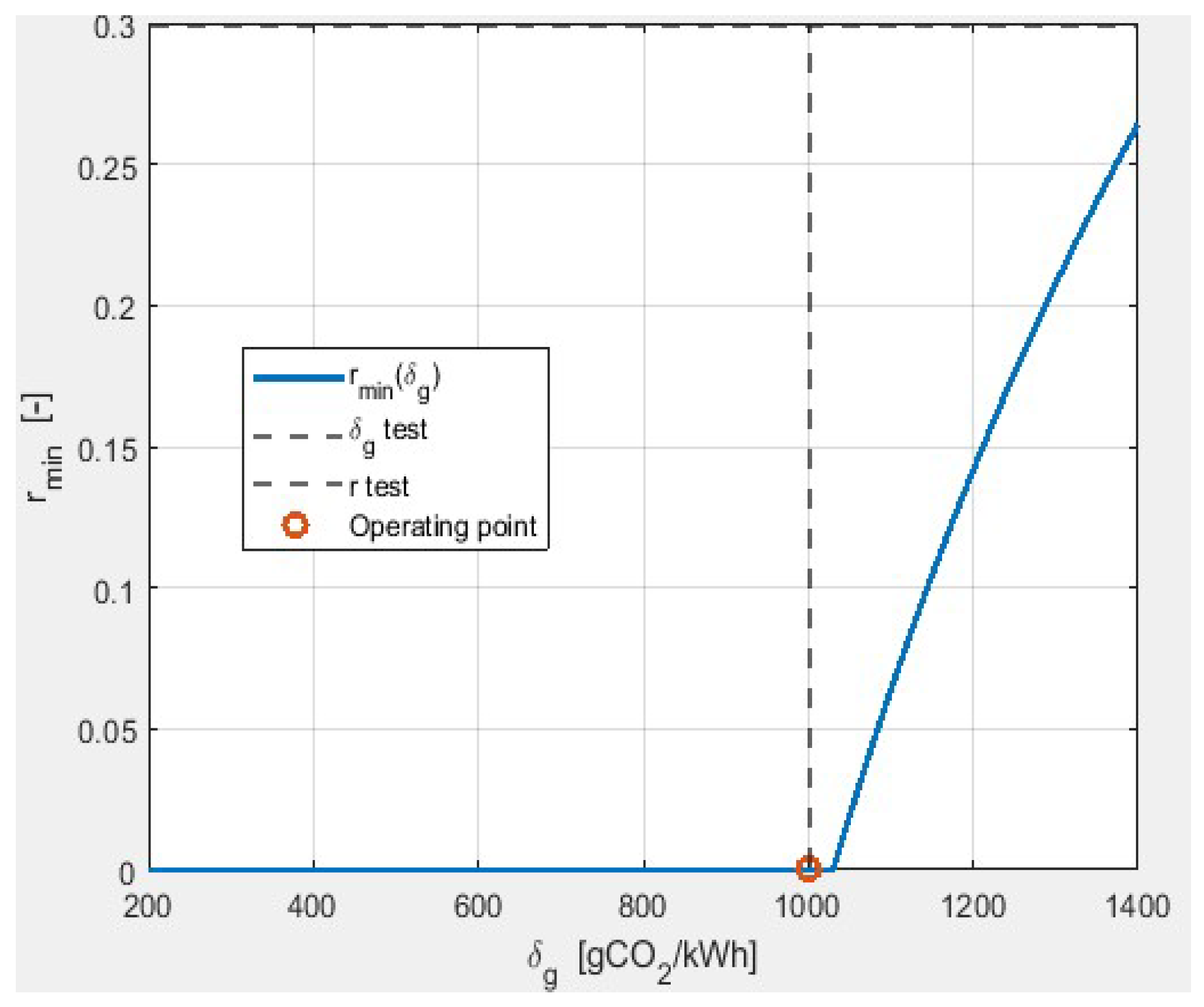
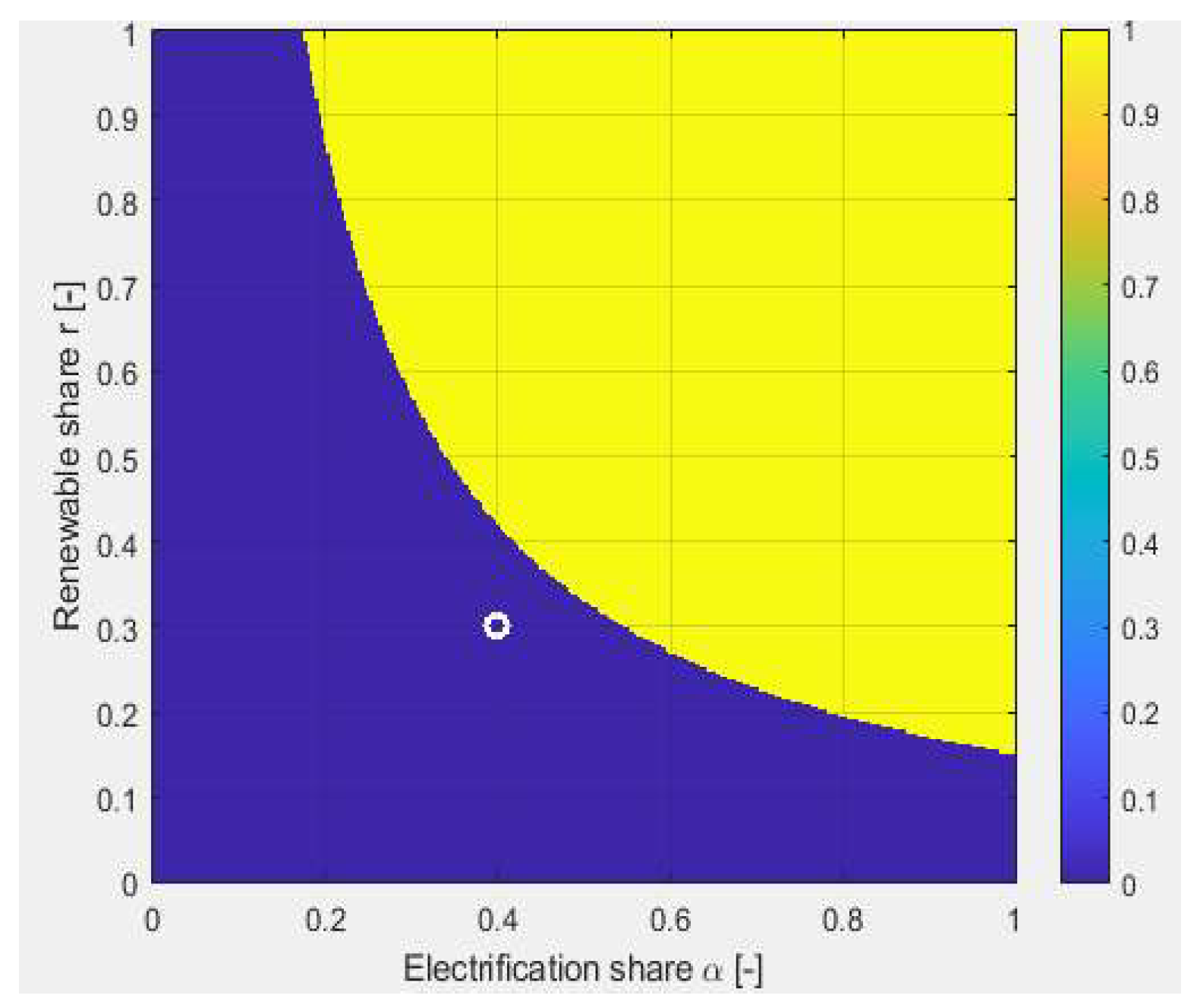
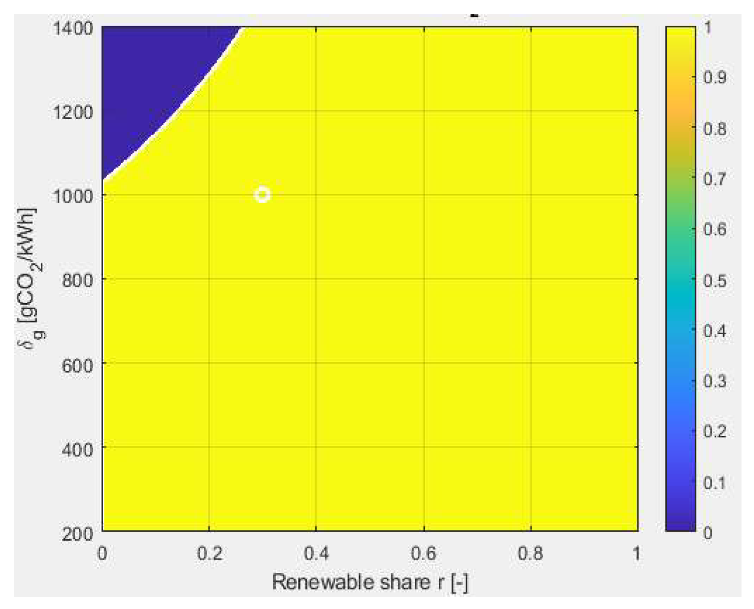
Figure 3 and Figure 4 represent the feasibility maps for $(r,{\delta }_g)$ and $(\alpha ,r)$ planes respectively. In both figures, the yellow region indicates the feasible domain where the corresponding condition is satisfied, while the blue region represents the infeasible domain where the condition is violated. Especially in Figure 3, the feasible (yellow) region corresponds to operating conditions where EV emissions are lower than ICEV emissions (${ϵ}_{EV}\le {ϵ}_{ICEV}$). In Figure 4, the feasible (yellow) region represents combinations of electrification share and renewable energy penetration for which the fleet-wide emission constraints are satisfied (${ϵ}_{fleet}\le {ϵ}_{cap}$).

Figure 3 is generated by evaluating the EV–ICEV emission condition over the $(r,{\delta }_g)$ space using the fleet emission formulation in Equation (4). For each pair of renewable share ($r$) and grid carbon intensity ${(\delta }_g)$ values, the condition defined by Equation (13) is assessed to determine wherever EV deployment results in lower emissions than ICEVs.

The feasibility region in Figure 3 (value = 1) corresponds to operating points where the inequality is satisfied, while infeasible regions (value = 0) indicate that EV emissions exceed those of ICEVs. The computation is performed using the emission factors provided in Table 3, and parameter ranges are systematically varied to construct the full feasibility map.

Figure 4 is obtained by evaluating the emission cap constraint over the $(\alpha ,r)$ space using the system-level emission formulation. For each combination of electrification share $\alpha$ and renewable share $r$, the fleet emission factor computed from Equation (4) is compared against the cap constraint defined by Equations (12) and (13). The white circular marker shown in Figure 4 corresponds to the representative baseline operating point adopted in this study, defined by an electrification share of ${\alpha }_{test}=0.40$ and a renewable-energy penetration of $r_{test}=0.30$. This operating point represents the initial user-defined planning scenario before optimization and sensitivity analysis. Its position within the feasible electrification region confirms that the selected operating condition satisfies the imposed emission and grid-capacity constraints under the adopted case-study assumptions.

Feasible regions (value = 1) correspond to operating points where the fleet emission remains below the specified cap ${ϵ}_{cap}$, while infeasible regions (value = 0) indicate violation of the constraint. The calculations are based on the emission parameters listed in Table 3 and evaluated scenarios summarized in Table 4.

The key observations from the above results are as follows:

• A large proportion of the $(r,{\delta }_g)$ space is infeasible for EV deployment under carbon-intensive grids.
• Increasing the electrification share α tightens the feasibility constraints, especially when emission caps are enforced.
• The feasible region shrinks rapidly for low renewable penetration, highlighting the system-level coupling between transport and the power sectors.

These results are consistent with previous scenario-based studies [19,39] but are now extended by providing continuous feasibility boundaries rather than discrete case comparisons.

4.2.3. Fleet Emission Surface and Sensitivity Analysis

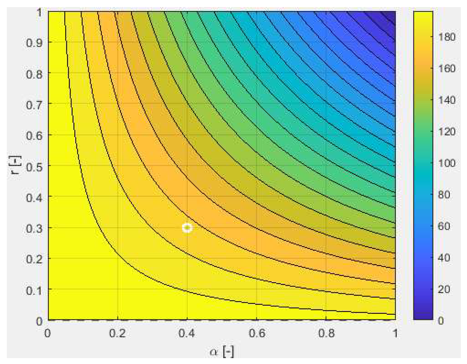
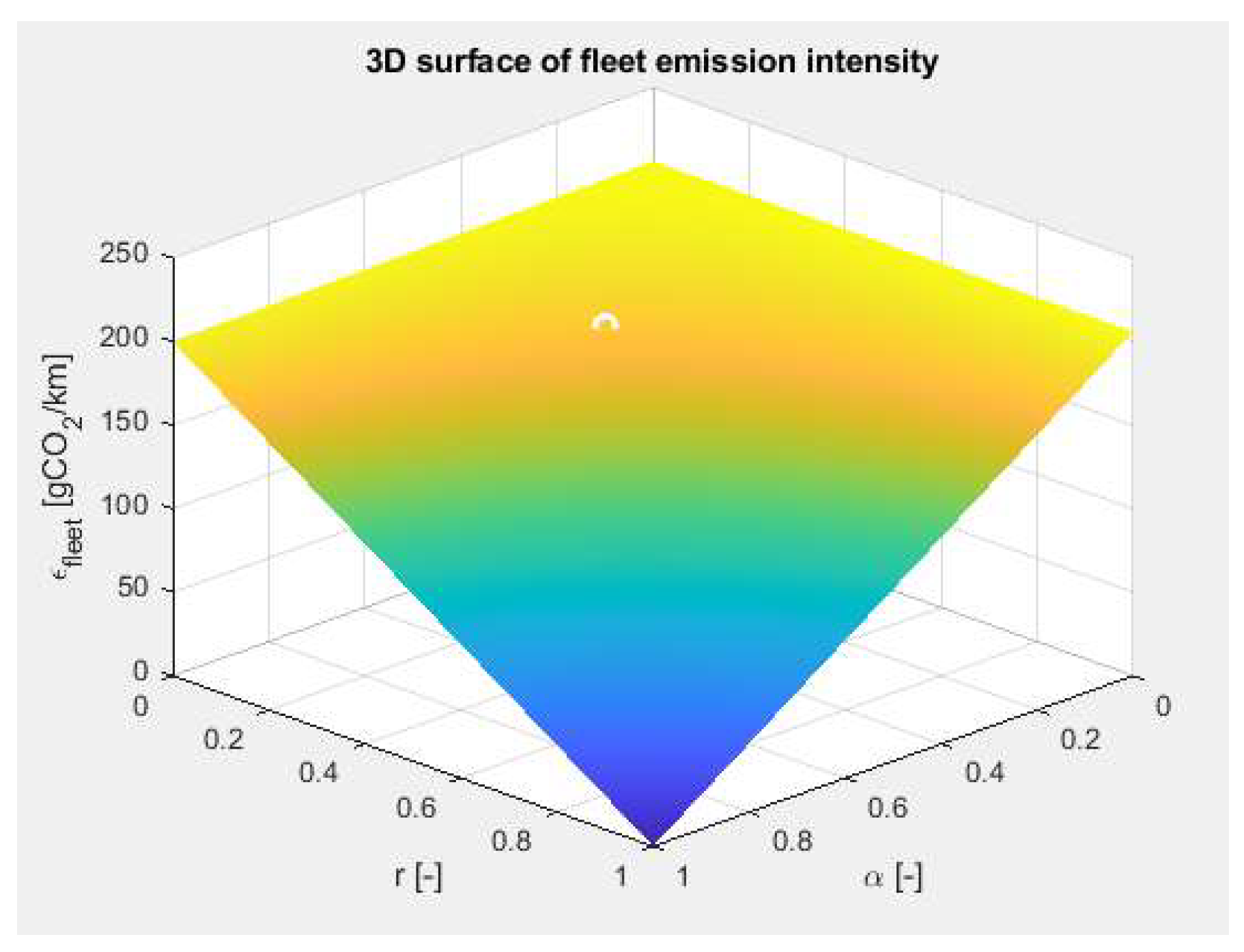
Figure 5 and Figure 6 depict the contour and surface plots of the fleet emission intensity ${ϵ}_{fleet}(\alpha ,r)$. The emission surface exhibits strong monotonic decrease with increasing renewable energy share $r$, and nonlinear sensitivity to electrification share $\alpha$ particularly at intermediate renewable levels.

Figure 5 is generated by evaluating the fleet emission formulation given by Equation (4) over a discretized grid of electrification share $\alpha$ and renewable share $r$. For each pair $(\alpha ,r)$, the fleet emission intensity ${ ϵ}_{fleet}\left(\alpha ,r\right)$ is computed using the emission factor defined in Table 3.

The contour line represents iso-emission levels, i.e., constant values of ${ ϵ}_{fleet}$, allowing visualization of the intensity of emissions to variations in $\alpha$ and $r$. The operating point $({\alpha }_{test},r_{test})$ shown by the white circular marker corresponds to the scenario defined in Table 4 and is superimposed for reference.

Figure 6 is obtained using the same dataset as Figure 5 by evaluating the fleet emission formulation in Equation (4) across the $(\mathsf{\alpha },\mathrm{r})$ space. The three-dimensional surface represents the variation in ${ϵ}_{fleet}$ as a function of electrification share and renewable penetration.

The surface illustrates the monotonic decrease in the fleet emissions with increasing renewable share $r$, as well as the nonlinear interaction between $\alpha$ and $r$. The plotted values are computed using the emission parameters listed in Table 3, and the highlighted operating point shown as a white circular marker corresponds to the evaluated scenario in Table 4.

4.2.4. Energy Demand, Renewable Capacity and Cost Implication

Figure 7, Figure 8 and Figure 9 analyze energy and economic impacts as functions of renewable share.

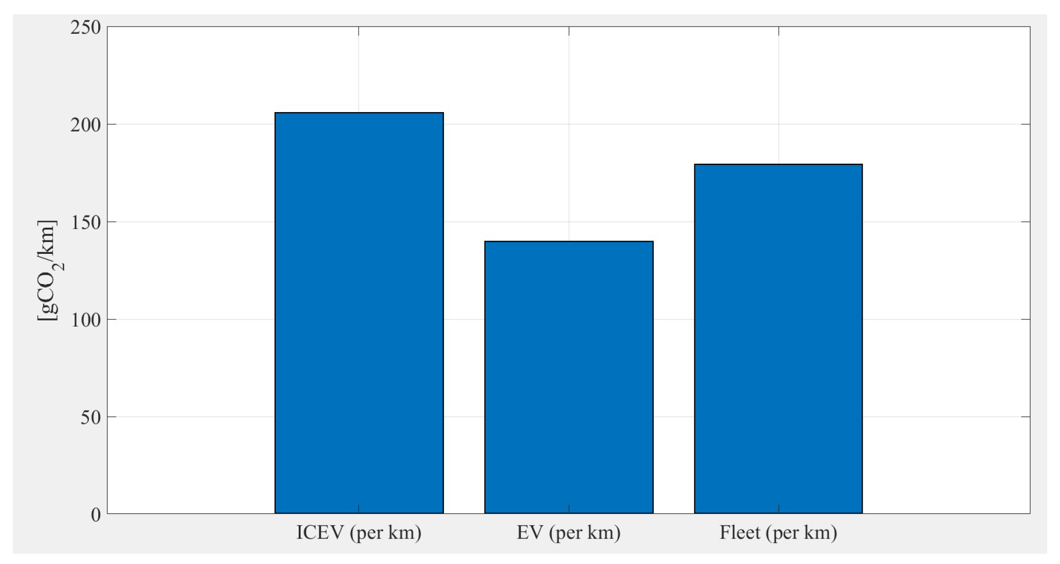
Figure 7 is defined by evaluating the emission expressions at the selected operating point $({\mathsf{\alpha }}_{test},{\mathrm{r}}_{test})$. The ICEV emission corresponds to the constant emission factor ${ϵ}_{ICE}$, while the EV emission is computed using the formulation in Equation (3). Fleet emission is calculated using the fleet-average expression given in Equation (4). All values are derived using the emission parameter listed in Table 3 and the operating conditions defined in Table 4. The comparison highlights the relative emission performance of each technology at the selected operating point.

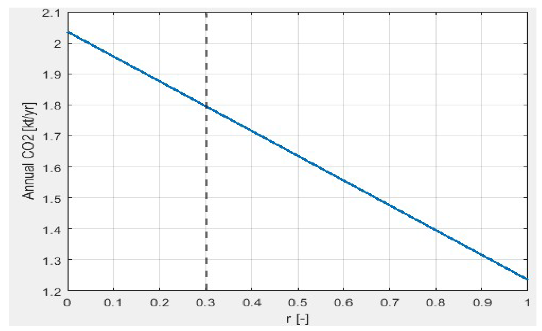
Figure 8 is generated by evaluating the annual emission formulation as a function of renewable share $\mathrm{r}$, while keeping the electrification share fixed at ${\mathsf{\alpha }}_{test}$. The annual emission is computed using the system-level formulation defined by Equation (9), based on the fleet emission intensity obtained from Equation (4).

The renewable share $\mathrm{r}$ is varied over its full range, and corresponding emission values are calculated using the parameters listed in Table 3. The vertical reference dashed line indicates the selected operating point ${\mathrm{r}}_{test}$, as defined in Table 4. The vertical reference dashed line shown in Figure 8 corresponds to the selected baseline renewable-share operating point $r_{test}=0.30$, as defined in Table 4. This reference value represents the renewable-energy penetration adopted for the representative case-study scenario prior to optimization and sensitivity analysis. The dashed line therefore provides a graphical indication of the baseline planning condition relative to the complete renewable-share sensitivity range investigated in the study.

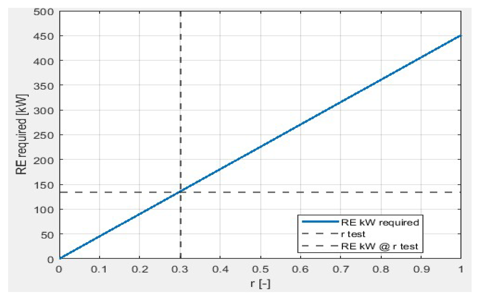
Figure 9 is obtained by evaluating the renewable energy requirement as a function of the renewable share $r$, for a fixed electrification level ${\alpha }_{test}$. The required renewable capacity is computed from the energy balance formulation given by Equation (14), which relates the total electrified demand to the unavailable generation capacity.

The renewable share $r$ is varied across its full range, and the corresponding required capacity is calculated using the system parameters defined in Table 4. The vertical dashed reference line shown in Figure 9 corresponds to the selected baseline renewable-share operating point $r_{test}=0.30$, while the horizontal dashed reference line represents the corresponding required renewable-generation capacity ${RE}_r$ necessary to sustain the selected electrification level under the adopted case-study assumptions. The intersection of these two dashed reference lines therefore identifies the baseline planning operating condition before optimization and sensitivity analysis. This graphical representation illustrates the direct relationship between renewable-energy penetration and the renewable-generation capacity required to support transport electrification.

The key observations from the above results are as follows:

• Total system cost exhibits a convex shape with respect to r, reflecting the trade-off between the carbon taxation and renewable capital investment.
• Renewable capacity requirement increases linearly with r.
• Minimum cost operating region does not necessarily coincide with the minimum emission region.

The above findings highlight the importance of multi-objective optimization, as cost-optimal and emission-optimal solutions differ substantially. This insight aligned with integrated planning studies such as [13,15,20].

Annual emission results obtained are identical because the effective renewable share equals the tested value $r_{eff}=r_{test}$, meaning that all emission metrics are evaluated under the same operating condition. Consequently, the annual fleet emission (basic), annual fleet emission (total), and annual CO₂ emission using $r_{eff}$ have the same value of 1.796 kT per year. On the other hand, the energy demand and renewable sizing results are summarized in

Table 6. Energy demand and renewable sizing.

Quantity	Description	Value
$E_{EV}$	EV electricity demand	8.696 × 105 kWh/year
$E_{RE,target}$	Target renewable energy	2.609 × 105 kWh/year
$P_{RE,req}$	Required renewable energy capacity	135.36 kW
Capacity Factor (CF)	CF for renewables	0.22
$P_{RE,used}$	Renewable energy capacity used	135.36 kW
$r_{eff}$	Achieved renewable share	0.3

.

The values reported in Table 6 are obtained from the energy balance and renewable sizing formulation. EV electricity demand $E_{EV}$ is computed from the annual travel demand and electrification share using the energy consumption model using the annual EV energy demand relationship derived from fleet electrification demand. The target renewable energy $P_{RE,Target}$ is then determined as a fraction of this demand based on the renewable share $r_{test}$.

The requested renewable capacity $P_{RE,req}$ is calculated using the relationship between annual energy and installed capacity given by Equation (14), which incorporates the capacity factor (CF). The renewable capacity used $P_{RE,used}$ corresponds to the available capacity under system limits, and the achieved renewable share $r_{eff}$ is obtained by comparing the actual renewable energy supplied to total EV energy demand. All values are evaluated at the operating point defined in Table 4.

4.2.5. Sensitivity Analysis Results and Discussion

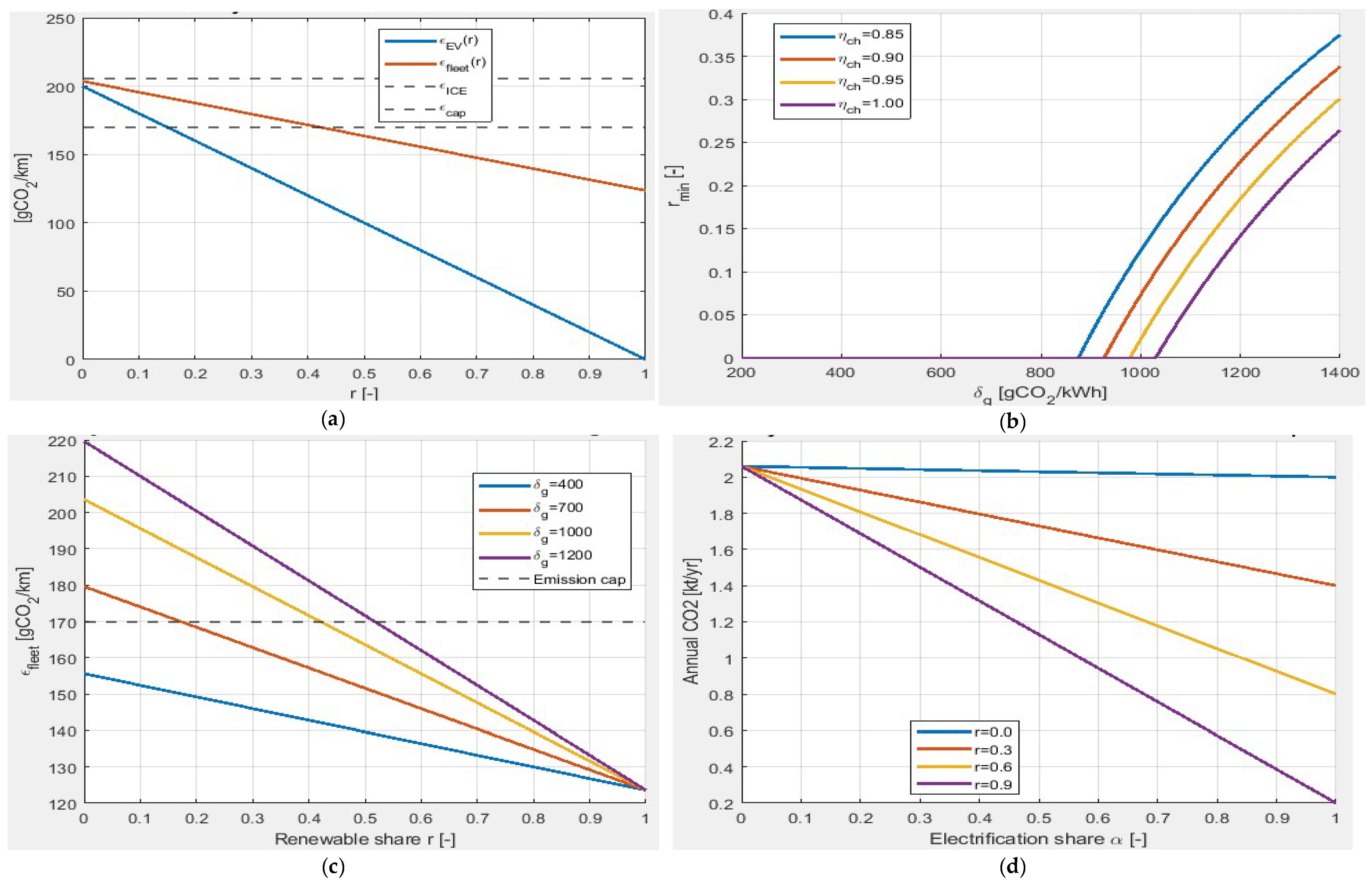
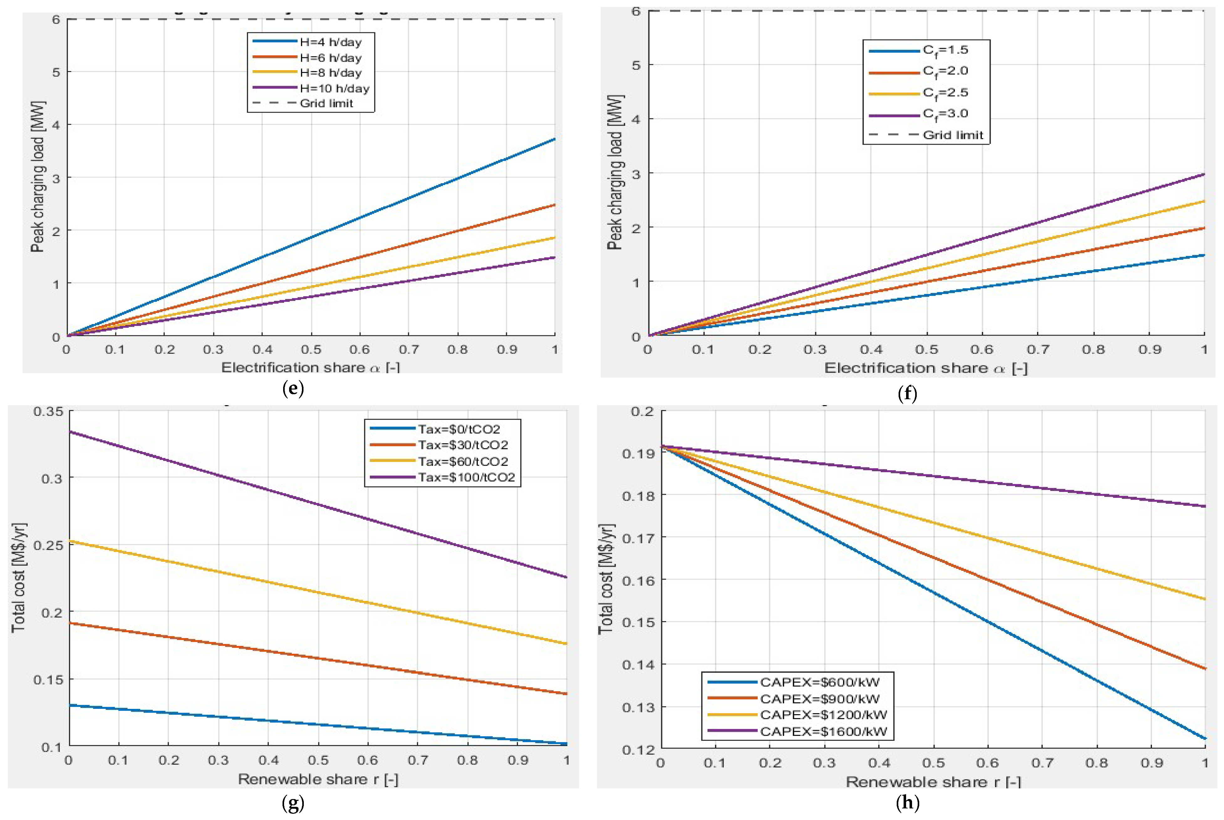
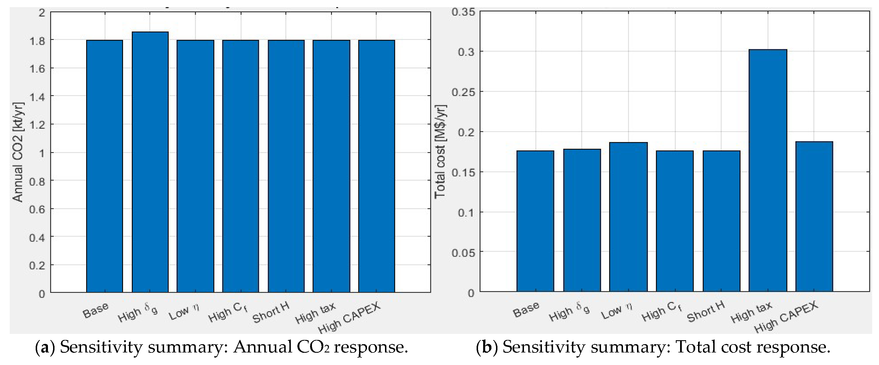
A comprehensive sensitivity analysis is conducted in this study to evaluate the robustness of the proposed analytical and optimization framework under variations in transport–energy system parameters, including grid carbon intensity, renewable energy penetration, charging efficiency, charging window duration, charging simultaneity, carbon taxation, and renewable energy investment cost. The results obtained are presented in Figure 10.

Figure 10a demonstrates that the EV emission declines linearly with $r$, and the fleet emission exhibits diminishing returns at high $r$ values due to residual ICEV and PHEV contributions. These trends confirm that electrification alone is insufficient without parallel decarbonization of the electricity supply, as emphasized in studies [1,4,8]. The curve in Figure 10a is generated by evaluating the emission formulations and functions of the renewable share $r$. The EV emission curve is obtained from the emission expression defined by Equation (2), while the fleet emission curve is computed using the fleet-average formulation in Equation (4), for a fixed electrification share $\alpha$.

The ICEV emission level is represented as a constant reference corresponding to ${ϵ}_{ICEV}$, and the emission cap is introduced using the constraint defined in Equation (12). The renewable share $\mathrm{r}$ is varied over its full range, and the corresponding emission values are calculated using the parameters listed in Table 3. The resulting plot illustrates the relative behavior of EVs, ICEVs, and fleet emissions under increasing renewable penetration. The horizontal dashed reference lines shown in Figure 10a represent the ICEV emission level ${ϵ}_{ICE}$, and the imposed emission-cap threshold ${ϵ}_{cap}$. These dashed reference lines provide graphical benchmarks for evaluating the reduction in EV and fleet-level emissions as renewable-energy penetration increases. Their intersections with the emission trajectories indicate the renewable-share conditions under which the corresponding electrification scenarios satisfy the imposed environmental constraints.

In terms of the sensitivity of the renewable cut-off threshold, Figure 10b illustrates the sensitivity of the minimum renewable share threshold $r_{min}$ to grid carbon intensity ${\delta }_{\mathrm{g}}$ under different charging efficiencies ${ \eta }_{ch}$. The results show that the renewable share required for EVs to achieve lower emissions than ICEVs increases substantially as grid carbon intensity increases. Under low-carbon electricity systems (${\delta }_{\mathrm{g}}<800 {\mathrm{g}}_{\mathrm{C}{\mathrm{O}}_2}/\mathrm{k}\mathrm{W}\mathrm{h}$), the cut-off condition remains weakly restrictive even at moderate charging efficiencies. However, under carbon-intensive grids, the required renewable penetration rises rapidly.

The analysis further demonstrates that charging efficiency has a significant influence on electrification feasibility. Lower charging efficiency increases indirect EV emissions because additional electricity generation is required to compensate for charging losses. Consequently, the required renewable share threshold shifts upward as charging efficiency decreases. For example, at ${\delta }_{\mathrm{g}}<1400 {\mathrm{g}}_{\mathrm{C}{\mathrm{O}}_2}/\mathrm{k}\mathrm{W}\mathrm{h}$, the required renewable share exceeds approximately 0.37 for ${\eta }_{ch}=0.85$, while it decreases to approximately 0.26 for ideal charging conditions (${\eta }_{ch}=1.0$). These results confirm that both grid decarbonization and charging efficiency improvement are essential for environmentally beneficial electrification under carbon-intensive electricity systems.

Figure 10c presents the variation in fleet emission intensity with renewable energy penetration under different grid carbon intensity scenarios. The results indicate that increasing renewable penetration consistently reduces fleet-level emissions across all electricity generation conditions. Under low-carbon grids (${\delta }_{\mathrm{g}}<400 {\mathrm{g}}_{\mathrm{C}{\mathrm{O}}_2}/\mathrm{k}\mathrm{W}\mathrm{h}$), the fleet emission intensity remains below the imposed emission cap threshold over the entire renewable share range, indicating favorable electrification conditions. The horizontal dashed reference line shown in Figure 10c represents the imposed fleet-emission cap ${ϵ}_{cap}$. This reference line provides a graphical indication of the admissible environmental boundary used to evaluate whether the fleet-emission trajectories under different grid carbon-intensity conditions satisfy the imposed emissions constraint. The intersections between the emission trajectories and the dashed cap line identify the minimum renewable-share levels required to maintain fleet emissions below the allowable threshold.

In contrast, highly carbon-intensive grids (${\delta }_{\mathrm{g}}<1000-1200 {\mathrm{g}}_{\mathrm{C}{\mathrm{O}}_2}/\mathrm{k}\mathrm{W}\mathrm{h}$) with low renewable penetration produce fleet emissions substantially above the emission cap boundary. However, increasing renewable penetration progressively reduces the fleet emissions until convergence occurs near fully renewable charging conditions. The results therefore confirm that renewable energy deployment acts as a structural enabling condition for large-scale electrification and that electrification without simultaneous grid decarbonization may fail to produce meaningful emission reductions.

Figure 10d illustrates the variation in annual CO₂ emissions with electrification share for different renewable energy penetration levels. The results reveal that electrification alone does not guarantee substantial emission reduction when renewable penetration remains low. At r = 0, increasing electrification produces only marginal emission reduction because EV charging remains strongly dependent on fossil fuel-based electricity generation. Conversely, under high renewable penetration (r = 0.9), increasing electrification significantly reduces total annual emissions, demonstrating strong coupling between renewable deployment and electrification effectiveness. The analysis further indicates that the slope of the CO₂ reduction trajectory becomes steeper as renewable penetration increases, confirming that renewable energy integration amplifies the environmental benefit of electrification.

Figure 10e and Figure 10f present the sensitivity of peak charging demand to charging window duration and charging coincidence factor, respectively. Figure 10e shows that shorter charging windows substantially increase peak charging demand because the total charging energy becomes concentrated over shorter time intervals. For example, the peak charging load under a 4 h/day charging window is significantly larger than under a 10 h/day charging window for the same electrification share. These results demonstrate that charging coordination and load spreading can substantially improve grid feasibility without changing total annual electricity demand. Similarly, Figure 10f indicates that charging simultaneity represented by the coincidence factor $C_f$ strongly influences peak network loading. Highly synchronized charging behavior ($C_f=3.0$) produces substantially higher peak charging demand than coordinated charging behavior ($C_f=1.5$). The results therefore confirm that charging-management strategies and smart-charging coordination may significantly enlarge the feasible electrification region while reducing required grid reinforcement. The horizontal dashed reference lines shown in Figure 10e,f represent the maximum admissible grid-capacity limit adopted in the charging-demand analysis. These reference boundaries are used to evaluate whether the peak EV charging demand associated with different charging-window durations and charging coincidence factors remains within the allowable network hosting capacity. In Figure 10e, the intersections between the charging-demand trajectories and the dashed grid-capacity limit identify the maximum feasible electrification levels under different charging-duration scenarios. Similarly, in Figure 10f, the intersections between the charging-demand curves and the dashed capacity boundary indicate the maximum feasible electrification share that can be supported under varying charging simultaneity conditions without exceeding the available grid hosting capacity.

Figure 10g illustrates the sensitivity of total annual system cost to renewable penetration under different carbon tax levels. The results indicate that higher carbon taxation shifts the economic operating region toward lower-emission electrification pathways. Under zero carbon taxation, the total system cost remains comparatively low because fossil fuel-intensive electricity and ICEV operation are not penalized economically. However, increasing carbon taxation progressively increases the economic attractiveness of renewable-supported charging and low-emission electrification scenarios. The analysis therefore confirms that carbon pricing can act as a strong economic driver for coordinated renewable energy deployment and transport electrification.

Figure 10h presents the influence of renewable energy capital expenditure on total annual system cost. The results indicate that higher renewable energy investment cost increases the economic burden associated with deep decarbonization pathways.

Nevertheless, despite increased renewable CAPEX, the system still benefits environmentally from higher renewable penetration because the emission reduction obtained from cleaner electricity generation compensates for the additional investment cost from a long-term sustainability perspective. The results therefore demonstrate the existence of an economic–environmental trade-off between renewable infrastructure investment and transport sector decarbonization.

Figure 11a,b summarize the global sensitivity response of annual CO₂ emissions and total system cost under multiple perturbation scenarios. The results show that high grid carbon intensity increases emissions significantly, low charging efficiency moderately increases emissions and operational cost, larger coincidence factors and shorter charging windows primarily affect grid feasibility rather than annual emissions, higher carbon taxation strongly increases total system cost while promoting low-emission operating regions, and higher renewable energy CAPEX increases the cost associated with deep decarbonization strategies.

Overall, the completed sensitivity analysis confirms that the proposed framework remains qualitatively robust under moderate parameter variations. However, the quantitative values of the renewable share threshold, admissible electrification region, peak charging demand, and Pareto-optimal operating points remain strongly dependent on regional grid conditions, renewable availability, charging behavior, and economic policy assumptions.

4.2.6. Optimization Results

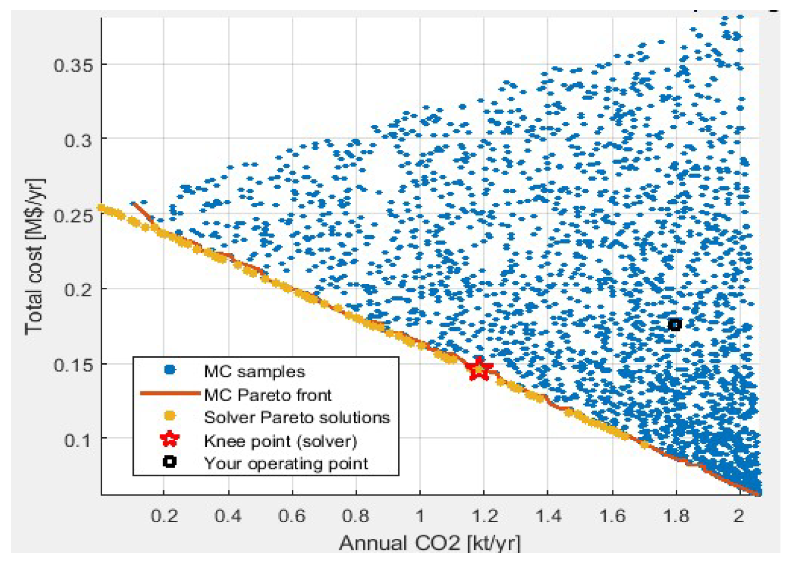
Figure 12 presents the Pareto front obtained from Monte Carlo sampling of $(\alpha ,r)$. It graphically shows the Monte Carlo solution, solver-derived Pareto front, knee point solution and the user-defined operating point. The resulting Pareto frontier clearly illustrates the fundamental trade-off between annual CO₂ emissions and total system cost when electrification, renewable energy integration, and grid constraints are considered together. Solutions with lower emissions are generally associated with the higher system costs, while cost minimal solutions tend to exhibit higher carbon footprints, confirming the necessity of a multi-objective planning approach.

The Pareto-optimal solutions obtained should therefore be interpreted as planning-level optimal operating regions derived under representative average system conditions rather than exact time-resolved operational dispatch solutions.

Relative to the user-defined operating point, the Pareto-optimal knee point solution achieves substantial annual CO₂ emission reduction while maintaining moderate total system cost increase within the admissible planning region. The minimum-emission operating region is associated with significantly higher renewable deployment and infrastructure investment requirements, whereas the minimum-cost region exhibits comparatively higher operational emissions and lower renewable penetration. These results quantitatively demonstrate the inherent trade-off between economic affordability, renewable energy integration, and transport sector decarbonization under coupled grid capacity constraints.

Wide dispersion of the non-dominated solution along the Pareto front indicates substantial flexibility in achieving feasible planning strategies, allowing policymakers to select solutions aligned with local priorities and constraints. In contrast, the user-defined operating point is frequently dominated by the Pareto-optimal solutions, revealing untapped improvement potential in commonly adopted electrification targets. Relative to the representative operating point $({\alpha }_{test}=0.4,{ r}_{test}=0.3)$, the identified knee point solution achieves approximately 34.2% lower annual CO₂ emissions while requiring increased renewable energy deployment and moderate additional system cost. Conversely, the minimum-cost operating region exhibits lower renewable penetration and reduced infrastructure investment but significantly higher operational emissions. The minimum-emission operating region achieves the largest emission reduction but requires substantially higher renewable capacity allocation and associated capital expenditure, thereby illustrating the economic–environmental trade-offs inherent in large-scale transport electrification planning.

Compared to deterministic scenario-based analysis, the Monte Carlo approach captures uncertainty and diversity across the feasible solution space, leading to more robust planning insights. The integrated visualization in Figure 11 provides a comprehensive decision support view. This unified representation facilitates benchmarking of existing strategies, identification of optimal and near-optimal solutions, and transparent communication of the cost emission trade-offs.

Figure 12 also indicates how the Pareto front obtained using the gamultiobj solver compares to Monte Carlo sampling. The key observations are listed below:

• The solver yields a smoother and denser Pareto front.
• Extreme solutions correspond to minimum emission and minimum cost regime.
• A knee point solution is clearly identifiable.

The identified knee point solution corresponding to renewable share r = 0.9832 represents a balanced transition operating condition where additional emission reductions beyond this point require disproportionately larger economic investment. The knee point therefore defines a practically attractive compromise between environmental performance and economic feasibility, making it particularly relevant for long-term transport–energy planning. In policy terms, this operating point suggests that substantial fleet decarbonization can be achieved through coordinated renewable deployment and partial electrification without necessarily requiring immediate full fleet electrification under carbon-intensive grid conditions.

The knee point solution presented in

Table 7. Knee point solution obtained from Pareto front.

Parameter	Value
Electrification share $(\alpha$)	0.4330
Renewable share $(r$)	0.9832
Annual CO2 emissions	1.1826 kT/year
Total system cost	0.146 M$/year

offers a practical balanced planning recommendation by achieving substantial emission reductions without disproportionate increases in the system cost. This solution is particularly relevant for policymakers seeking cost-effective decarbonization pathways.

The values reported in Table 7 are obtained from multi-objective optimization process described in Section 3.4.2. The optimization simultaneously minimizes annual CO₂ emissions and total system cost using the formulations defined in Equation (9) and the cost model. The Pareto front is generated using the Matlab generic algorithm solver gamultiobj, where each solution represents a trade-off between emission and cost.

The knee point solution is selected from the Pareto front as the point providing the best compromise between the two objectives, corresponding to the region of maximum curvature. The associated decision variables, namely the electrification share $\alpha$ and renewable share $r$, are directly extracted from this solution, while the corresponding emission and cost values are computed using the system-level formulations. The reported values therefore represent the optimal balanced operating point identified by the algorithm.

Table 8. Multi-objective optimization summary (GA-based).

Parameter	Value
Optimization method	gamultiobj
Decision variables	2
Nonlinear constraints	2
Generations	120
Function evaluations	24,001
Final average Pareto distance	0.0030
Final Pareto spread	0.1137
Termination reason	Maximum generations reached

summarizes the optimization results. The summarized results are obtained from the multi-objective optimization procedure implemented using the Matlab genetic algorithm solver gamultiobj. The problem is formulated using two decision variables, namely the electrification share $\alpha$ and the renewable share $r$, and two nonlinear inequality constraints responding to the emission cap and renewable capacity limits as defined by Equations (12)–(14).

The optimization is executed over the predefined number of generations, where each function evaluation corresponds to the computation of the objective functions, including annual CO₂ emissions (see Equation (9)) and total system cost. The final average Pareto distance and spread quantify the convergence and diversity of the obtained Pareto front. The termination condition indicates that the algorithm stopped upon reaching the maximum number of generations, and the reported value reflects the final optimization performance.

4.2.7. Peak Charging Load and Grid Constraint Analysis

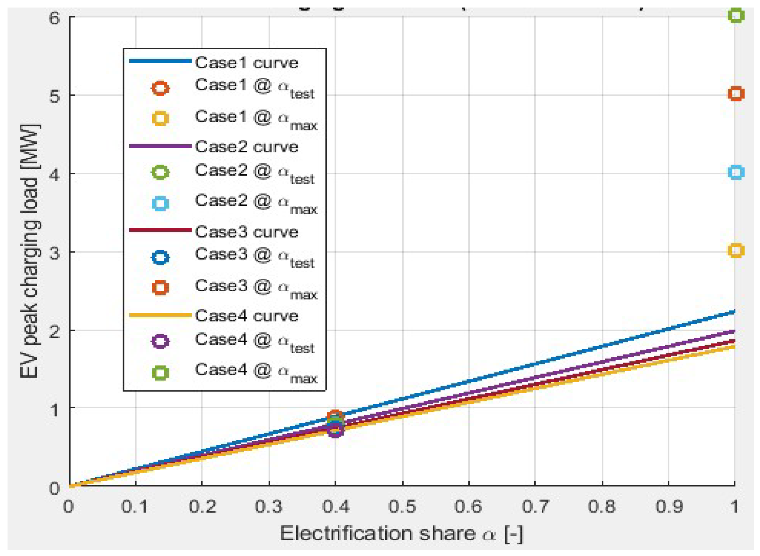
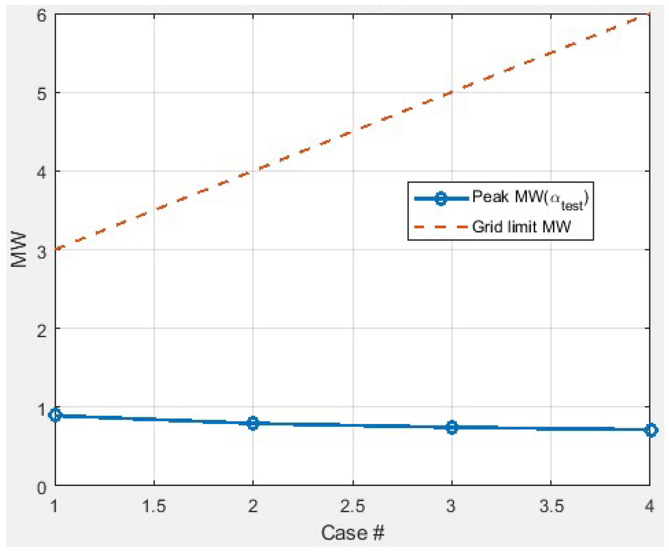
Figure 13 and Figure 14 present the analyses of the impact of the charging behavior on grid peak load.

Figure 13 is generated by evaluating the peak charging load formulation as a function of the electrification share $\alpha$ for the different charging scenarios defined in Table 2. The average EV charging power is computed using Equation (23), and the corresponding peak charging demand is obtained using Equation (24). Each curve corresponds to a particular charging scenario characterized by $H_{chg/day}$ and $C_f^{peak}$. The colored solid lines represent the peak EV charging load as function of $\alpha$, while the circular markers indicate the operating point ${\alpha }_{test}$ for each case. The variation across cases reflects the impact of charging duration and coincidence factors on peak demand.

$$P_{EV}={\displaystyle \frac{E_{EV}}{H_{chg/day}}}$$

(23)

$$P_{peak}=C_f\cdot P_{EV}$$

(24)

Figure 14 is obtained by evaluating the peak EV charging load at the operating point ${\alpha }_{test}$ for each scenario defined in Table 2. The peak load values are computed using the same formulation as in Figure 13, based on Equations (23) and (24), and are compared against the corresponding grid capacity limits $P_{grid,max}$.

In Figure 13, for each case, the parameters $H_{chg/day}$, $C_f^{peak}$ and $P_{grid,max}$ from Table 2 are used to compute the corresponding peak charging curves. The blue circular markers connected by a solid line indicate the peak EV charging power evaluated at the operating point ${\alpha }_{test}$ for each case, whereas the red dashed line represents the maximum grid capacity limits for each scenario. The markers therefore highlight the operating condition, while the dashed line defines the system constraint.

The comparison of the above two figures illustrates whether the charging demand remains within grid constraints for each case, thereby validating the feasibility of the selected operating point under different charging durations and coincidence factors.

The results demonstrate the following:

• Peak EV charging power scales linearly with the electrification share α.
• Shorter charging windows and higher coincidence factors significantly increase peak demand.
• Grid constraints impose strict upper bounds on allowable electrification levels.

Although the charging scenarios adopted in this study are based on representative planning-level charging behavior reported in the prior EV–grid integration literature, the resulting peak demand trends remain consistent with observed feeder-level hosting-capacity limitations reported in practical distribution network studies. The analysis therefore provides a scalable approximation of electrification-induced grid stress suitable for strategic planning assessment, while acknowledging that detailed feeder-specific studies would be required for operational deployment and localized infrastructure design. Future validation using feeder-level network datasets, chronological charging measurements, and distribution system power-flow simulations would further strengthen the applicability of the proposed framework under practical operational conditions.

The aforesaid multi-case analysis shows that the behavioral and operational factors such as charging duration and simultaneity can be as critical as total energy demand. This supports the findings in [5,16,17].

While Section 4.1 quantified system performance and trade-offs, the next section translates the findings into policy and planning implications, addressing how regulators and planners can operationalize the proposed framework.

4.3. Policy and Planning Implication

The results presented in Section 4.2 provide several important insights for policymakers, regulators, and system planners responsible for transport electrification, power system decarbonization and climate policy design. Unlike scenario-based studies, the proposed framework enables quantitative, system consistent policy evaluation, directly linking electrification targets to grid emissions, renewable integration, costs and infrastructure constraints.

4.3.1. Electrification Target Should Be Conditional and Not Absolute

A key policy implication of the present study is that the EV adoption target should not be defined independently of the grid carbon intensity. The analytical cut-off condition derived in Section 3.3 demonstrates that EV deployment can increase emissions if the renewable share of the electricity is below the threshold.

These findings challenge simplistic electrification mandates and support conditional EV incentives tied to grid decarbonization progress and region-specific electrification pathways rather than uniform national targets.

Such conditional policies align with prior observations in [3,5,31] and this work provides a quantifiable and operational rule for implementation. In practical terms, the proposed cut-off formulation can assist policymakers in defining minimum renewable energy deployment targets required before large-scale EV adoption programs are environmentally beneficial under specific grid carbon intensity conditions. The framework therefore supports region-specific electrification roadmaps based on measurable power system decarbonization progress rather than fixed uniform electrification mandates.

4.3.2. Carbon Tax Design and Transport Electrification

The integration of carbon pricing into the cost emission framework reveals that carbon taxes significantly influence the cost-optimal electrification trajectory. The policy relevant insight includes the following:

• Carbon taxation shifts the Pareto frontier toward the higher renewable share and lower emissions.
• Uniform carbon taxes applied only to the power sector may distort electrification incentives.
• Coordinated carbon pricing across transport fuels and electricity generation is essential.

The sensitivity analysis further indicates that increasing carbon tax levels progressively shifts Pareto-optimal operating regions toward lower-emission electrification pathways, thereby accelerating economically feasible transport decarbonization under renewable-constrained grid conditions. These results support the need for integrated tax design, as discussed in [2,12,13,34], while extending the application to transport electrification planning.

4.3.3. Renewable Energy as an Enabling Policy Instrument

The analysis presented in this study confirms that renewable energy deployment is not merely complementary but structurally necessary for emission effective electrification. From the policy standpoint,

• Renewable capacity expansion determines the feasible electrification envelope.
• Subsidies for renewable generation can indirectly accelerate transport decarbonization.
• Delayed renewable investment increases the cost of achieving emission targets.

This reinforces the argument in studies reported in [6,17,29] and highlights the importance of joint renewable–EV policy frameworks rather than isolated incentive schemes.

4.3.4. Grid Capacity and Charging Behavior Regulation

Peak load analysis reveals that charging behavior is a critical regulatory lever, in which the key implications include the following:

• Grid constraints can limit electrification more severely than energy availability.
• Uncoordinated charging may violate network limits even at moderate EV penetration.
• Time of use tariffs, smart charging mandates, and demand response programs are essential.

The proposed framework additionally enables planners and utilities to estimate admissible electrification levels under different charging-management strategies and available hosting-capacity conditions, thereby supporting phased charging infrastructure deployment and targeted grid reinforcement planning. These findings echo the concerns raised in [5,15,16] but extend them by quantifying maximum admissible electrification shares under explicit peak constraints.

4.3.5. Decision Support for Long-Term Planning

Combined Pareto analysis provides a powerful planning tool for policymakers and utilities. In particular,

• The knee point solution offers a rational compromise between cost and emissions.
• Policymakers can identify solutions that deliver most emission benefits at moderate cost.
• The framework supports transparent evaluation of trade-offs under uncertainty.

This type of decision support capability is largely absent from existing policy analyses and represents a practical contribution to strategic planning.

4.3.6. Implications for Carbon-Intensive Power Systems and Economic Planning

The results of the case study presented here are especially relevant for regions with coal-dominated electricity generation, rapidly growing vehicle fleets, and constrained grid infrastructure.

In such contexts, premature electrification without renewable expansion may increase emissions, validating the concerns raised in [1,3,4]. The proposed framework enables these regions to sequence electrification and decarbonization optimally, avoiding counterproductive outcomes. Accordingly, the results support phased transport electrification strategies in which renewable energy expansion, charging infrastructure deployment, and grid capacity reinforcement are coordinated progressively according to regional infrastructure readiness and electricity system carbon intensity. The proposed framework therefore enables utilities, regulators, and policymakers to identify economically feasible decarbonization pathways that coordinate renewable deployment, charging infrastructure expansion, and electrification targets according to regional grid-readiness conditions.

Overall, the findings emphases that effective transport decarbonization requires the following:

• Integrated planning across transport, electricity, and climate policy.
• Alignment between electrification incentives, renewable deployment and grid regulation.
• Quantitative tools capable of evaluating system-wide interactions.

The proposed methodology provides a foundation for such integrated policy design and can be adapted to different national or regional contexts. The framework may therefore assist policymakers, utilities, and transport planners in identifying when electrification should be accelerated, delayed, or regionally adapted according to renewable energy availability, grid capacity limitations, and carbon intensity conditions, thereby reducing the risk of environmentally counterproductive electrification pathways.

In addition to the environmental implications, the proposed framework also provides quantitative insight into the economic impacts associated with transport electrification under grid and renewable energy constraints. The annual system cost components corresponding to the evaluated operating point are summarized in

Table 9. Annual system cost breakdown at selected operating point $({\alpha }_{test},r_{test}).$

Cost Component	Equation Used	Annual Cost ($/year)
Grid electricity cost	Energy Balance (Section 3)	91,304.35
Renewable energy cost	Energy Balance (Section 3)	15,652.17
Carbon tax	Equation (9)	53,880.00
Renewable CAPEX (annualized)	Equation (14)	12,408.22
Renewable O&M	Equation (14)	2436.52
Total system cost		175,681.26

.

The estimated annual system cost presented in Table 9 remains sensitive to electricity price fluctuations, renewable energy investment assumptions, charging infrastructure deployment costs, and carbon pricing mechanisms. Consequently, the reported values should be interpreted as representative planning-level estimates rather than fixed universal costs. Variations in energy market conditions, financing assumptions, technology learning rates, and renewable deployment costs may significantly influence the economic attractiveness of alternative electrification pathways under different regional conditions.

The results in Table 9 correspond to a representative case study based on the selected operating point $\left({\alpha }_{test}=0.4, r_{test}=0.3\right)$ and system parameters defined in Table 2. The case study reflects a typical EV integration scenario in which annual energy demand, renewable penetration, and cost parameters are evaluated using the proposed framework.

The cost components are computed using the system-level formulations, where the grid electricity cost is obtained from the residual energy demand not supplied by renewables, the renewable energy cost is derived from the allocated renewable share (as summarized in Table 7), and the carbon tax is calculated based on the total CO₂ emissions defined by Equation (9). The renewable CAPEX and O&M costs are determined from the required installed capacity computed in Equation (14), using standard cost coefficients. The total system cost reported in Table 9 is then obtained as the sum of all individual cost components.

The optimal electrification share α = 0.4330 obtained from the knee point solution indicates that partial fleet electrification may represent the most economically and environmentally balanced transition pathway under the assumed grid carbon intensity and renewable energy availability conditions. The results further suggest that aggressive electrification without parallel renewable energy deployment and grid capacity reinforcement may lead to diminishing environmental returns and increased system costs. Consequently, the proposed framework supports phased and grid-aware electrification strategies in which renewable deployment, charging infrastructure expansion, and transport electrification are coordinated simultaneously.

To synthesize the proposed framework, and its underlying interactions, Figure 14 presents a comprehensive system-level representation of the electrification process, illustrating the relationships between energy sources, vehicle technologies, emission pathways, and economic outcomes. Figure 15 highlights how grid carbon intensity, renewable energy integration, and fleet composition jointly influence total emissions and system costs under the defined constraints.

The colors used in Figure 15 represent the different physical subsystems, energy pathways, emission contributions, and information exchanges within the integrated transport-electrification framework. The blue elements and arrows correspond to grid electricity supply, electrical energy flow, and interactions related to electricity generation and charging demand. The green elements and arrows represent renewable energy integration, including renewable energy penetration, renewable capacity contribution, and renewable energy supply to EV charging. The red elements and arrows denote ICEV-related emission contributions and conventional fossil-fuel transport pathways, whereas the orange elements and arrows correspond to PHEV-related emission pathways and hybrid electrification contributions. The purple dashed arrows indicate information exchange, optimization coupling, and dependency relationships between the fleet-emission model, environmental outcomes, economic outcomes, and operational constraints. Together, these color-coded flows visually illustrate the coupling between grid carbon intensity, renewable-energy deployment, electrification share, fleet emissions, charging demand, economic performance, and system-level operational constraints within the proposed analytical framework.

5. Conclusions and Recommendations

This study presented an integrated analytical and optimization-based framework to assess the environmental, economic, and infrastructural implications of EV deployment under heterogeneous grid and policy conditions. By explicitly coupling vehicle electrification, renewable energy integration, carbon pricing and grid capacity constraints, the proposed methodology advances beyond conventional scenario-based assessments and provides a unified decision support tool for transport and energy system planning.

The results demonstrated that EV adoption is not universally emission beneficial. A closed form cut-off condition was derived showing that EVs reduce fleet-level CO₂ emissions only when the renewable share of electricity exceeds a grid-dependent threshold. Below this threshold, electrification may increase emissions relative to ICEVs. This finding highlighted the fundamental dependence of transport decarbonization outcomes on power system characteristics and reinforces the need for coordinated planning across sectors.

The analysis further revealed that electrification share and renewable allocation jointly determine fleet emission intensity, creating strong structural coupling between transport and electricity systems. Increasing electrification without sufficient renewable integration yields diminishing environmental benefits and can even be counterproductive. This coupling was shown to persist under both cost-minimizing and emission-minimizing objectives, emphasizing that electrification policies cannot be designed in isolation from power sector decarbonization strategies.

Economic evaluation indicated that cost and emission objectives are inherently conflicting. Multi-objective optimization revealed a well-defined Pareto front, with minimum cost and minimum emission solutions occupying distinct regions of the decision space. More importantly, automatically identified knee point solutions were shown to provide a practical compromise, achieving substantial emission reduction at moderate additional cost. Such solutions are relevant for policymakers seeking balanced and politically feasible decarbonization pathways.

A key contribution of this work lies in the explicit treatment of the grid peak constraints. The peak charging analysis demonstrated that charging behavior, coincidence factors and network capacity impose strict upper bounds on admissible electrification levels. In many cases these constraints were more restrictive than energy availability or emission targets, underscoring the critical role of charging regulation and grid-aware planning in large EV deployment.

The proposed framework therefore provides a practical basis for phased transport electrification planning by identifying coordinated renewable deployment, charging infrastructure expansion, and grid capacity reinforcement strategies required to achieve environmentally beneficial electrification. The methodology further enables policymakers and utilities to evaluate when electrification should be accelerated, delayed, or regionally adapted according to power system carbon intensity and infrastructure readiness.

Despite its contributions, the study has some limitations. The analysis relies primarily on annual average representations of energy demand and emissions and therefore does not capture temporal variability such as seasonal renewable fluctuation or short-term network congestion. Furthermore, the grid representation adopted in this study is based on aggregate peak demand constraints and equivalent charging window formulations rather than detailed time-resolved power-flow analysis. Consequently, localized feeder congestion, voltage regulation issues, and short-term operational dynamics are not explicitly modeled. Incorporating chronological load curves, distribution network topology, and stochastic charging behavior represents an important extension for future work.

Charging behavior is modeled using parametric charging windows and coincidence factors rather than detailed stochastic agent-based representation.

The present framework represents EV charging demand using an aggregate planning-oriented formulation based on equivalent charging windows rather than explicit hourly chronological simulation, where charging demand is distributed over a representative charging duration $H_{chg}$ and converted into an equivalent peak charging load through the charging coincidence factor $C_f$, which approximates the degree of simultaneity among charging vehicles during peak demand periods. Higher values of $C_f$ correspond to highly synchronized charging behavior, such as uncontrolled evening charging, whereas lower values represent more diversified or partially coordinated charging conditions consistent with smart charging strategies. Consequently, the proposed methodology implicitly captures the effects of charging window duration, peak demand concentration, charging simultaneity, and coordinated charging behavior on grid loading and electrification feasibility. However, the framework does not explicitly model hourly charging trajectories, stochastic charging arrival patterns, dynamic electricity pricing, vehicle-to-grid interactions, or chronological renewable intermittency. Instead, the adopted aggregate representation is intended for strategic transport electrification planning and large-scale feasibility assessment while preserving analytical tractability within the proposed optimization framework. The vehicle heterogeneity and user-specific driving patterns are aggregated into representative parameters. Also, policy instruments such as carbon taxation and electricity pricing are treated as exogenous and uniform.

These limitations provide a natural direction for future studies. Extending the framework to time-resolved modeling would allow the incorporation of hourly charging profiles, renewable generation variability, and dynamic grid constraints. Inclusion of stochastic charging behavior and smart charging strategies would further enhance peak load assessment. Expanding the analysis to full lifecycle emissions, including vehicle manufacturing and battery degradation, would provide more comprehensive environmental perspectives. Coupling the proposed framework with detailed power system operation models could enable deeper insight into system-wide impacts, while policy-focused extensions could explore differentiated carbon taxes, dynamic tariffs, and targeted incentive schemes. Finally, applying the methodology to developing and coal-dominated power systems would further demonstrate its adaptability and relevance in diverse regional contexts.

The completed sensitivity analysis further demonstrated that grid carbon intensity, renewable energy penetration, charging efficiency, charging window duration, charging simultaneity, carbon taxation, and renewable energy investment cost constitute the dominant factors governing the environmental and economic feasibility of transport electrification. The results confirm that environmentally beneficial electrification requires coordinated renewable energy deployment, charging demand management, and grid-aware planning strategies, particularly under carbon-intensive electricity systems.

In conclusion, the present work contributes a novel, analytically grounded, and practically implementable framework for evaluating EV deployment within an integrated energy–transport climate context. By providing explicit feasibility conditions, optimization-based trade-off analysis and grid-aware planning metrics, the proposed approach supports informed decision making toward cost-effective and genuinely low-carbon mobility transition.