Stability Control of Vehicles with Brake Failure Based on the TD3 Adaptive Sliding Mode Control Algorithm

Abstract

To address the issue of vehicle instability and veering during braking when a single wheel fails in an electric vehicle’s electromechanical braking (EMB) system, an integrated application-oriented control framework based on adaptive sliding mode control (ASMC) is proposed. To address the shortcomings of SMC—such as difficulty in suppressing oscillations and the high workload associated with parameter tuning—a novel composite reaching law function was designed, and the TD3 algorithm was employed to optimize the sliding mode control parameters. When a failure in the EMB system is detected, the upper-layer control uses an improved ASMC algorithm to calculate the vehicle’s additional yaw moment. The lower-layer control employs an optimal control algorithm to distribute braking force, taking into account braking intensity, yaw moment, and tire utilization. This approach is integrated with sliding mode steering control to enhance vehicle stability during braking. To meet the driver’s braking requirements, a backpropagation (BP) neural network is first employed to identify braking intent. Based on this, the additional yaw moment is calculated by the upper-layer controller, and the brake force distribution is optimized through the lower-layer controller, thereby improving the vehicle’s stability. Through co-simulation analysis using Simulink-2024a and CarSim-2019.1, the results show that, compared to traditional algorithms, the proposed hierarchical control strategy reduced the maximum sideslip angle by 51.4%, decreased the maximum yaw rate by 47.2%, and reduced the maximum lateral offset by 45.6%. This control strategy enables enhanced stability across various braking intensity conditions.

1. Introduction

In recent years, new energy vehicles have been evolving toward intelligent integration. Within their braking systems, brake-by-wire systems are gradually replacing traditional hydraulic braking systems due to their faster response and lighter weight. Compared with electro-hydraulic braking (EHB) systems, the EMB system has become a key focus for researchers and enterprises worldwide because of its superior response speed and precise control capabilities [1,2].

Compared with the EHB system, the EMB system directly engages the brake caliper with the brake disc via an electric motor, enabling independent control of each wheel. This promotes enhanced handling stability and safety during vehicle operation [3]. However, due to its fully electronic nature, the EMB system lacks the traditional hydraulic backup found in EHB systems. A failure in the EMB system would lead to degraded braking performance [4]. Therefore, enhancing its fault tolerance has become a critical issue that urgently needs to be addressed in the development of this technology.

Extensive research has been conducted by scholars worldwide on the issue of failure in brake-by-wire systems. Reference [5] proposed a fault-tolerant control architecture for brake-by-wire vehicles. It integrated a regenerative braking system, first employing a sliding mode control algorithm to calculate the compensating yaw moment, then deriving the braking torque. This approach reduced the error between the controlled yaw rate and the desired yaw rate to less than 2°/s and minimized the speed control error to under 1 km/h. However, it did not address the issue of braking force reconstruction under high braking intensity conditions. Reference [6] proposed a fault-tolerant control algorithm employing an explicit weighted pseudoinverse distribution and redistribution mechanism. When an actuator failed, this approach required only the redistribution of signals generated by upper-layer controllers, without requiring reconfiguration of the control system. However, this control method showed limitations under heavy braking conditions. Reference [7] introduced a fault factor to quantify the severity of brake failures and employed a sliding mode controller to regulate the vehicle’s yaw moment, thereby reconstructing the braking force. Reference [8] proposed a two-layer controller using yaw rate and sideslip angle as state variables, where the inner layer employed model predictive control (MPC) and the outer layer utilized fuzzy proportional–integral–derivative (PID) control. Finally, the desired stability control was achieved through the distribution of four-wheel braking torque. Reference [9] proposed a nonlinear model predictive observer for vehicle trajectory tracking, which demonstrated improved control accuracy and computational efficiency compared to standard MPC controllers. Reference [10] introduced multiple enhancements to existing adaptive path-tracking controllers, improving tracking performance and disturbance rejection capabilities. In Reference [11], through broadcast control, the architecture transitioned from conventional centralized control to autonomous distributed control of braking and driving forces. When single-wheel or dual-wheel failures occurred, the vehicle maintained acceptable stability and performance through the autonomous distributed behavior of the remaining wheels.

In terms of vehicle stability control, Reference [12] proposed a method for achieving stable control by relying on the combined effect of the center yaw moment of the vehicle’s front axle and the center of gravity yaw moment. The upper-layer controller calculates the additional yaw moment required for the vehicle to maintain stability based on the vehicle’s state, while the lower-layer controller allocates the required yaw moment to the optimal driving torque of each wheel. Reference [13] proposed a joint sliding mode control algorithm combined with fuzzy adaptive gain to address the issue that lateral stability control of the vehicle during the steering state is affected by system parameter perturbations and external environmental disturbances. Additionally, a simplified unscented Kalman filter observer was proposed for the dynamic estimation of vehicle state parameters and the road adhesion coefficient, which can be used by the lateral stability controller. In terms of fault-tolerant control for braking failures, Reference [14] proposed an overall control architecture and first analyzed braking failure modes under various conditions. Subsequently, braking reconstruction rules were established to adjust the braking force on the remaining functioning actuators when a braking failure mode occurred. Moreover, the $H\infty$ algorithm was introduced to determine the reconstructed braking force based on the vehicle’s dynamic state. Reference [15] proposed a coordinated control method for fault-tolerant control of the braking actuator. The drive and braking controllers optimally distributed the required longitudinal force and yaw moment, and set constraints aimed at keeping the yaw moment error within the allowable range. The yaw moment deficit left by the drive and braking controllers was effectively compensated by the steering controller’s front and rear wheel feedforward steering angles.

Most of the aforementioned studies focused on single-wheel failure scenarios during straight-line braking, often overlooking the impact of different road surface friction coefficients on braking performance. Furthermore, these studies exhibited limitations such as slow controller response times and the use of overly simplistic objective functions for optimizing brake force distribution, making them less adaptable to complex operating conditions. In response to the nonlinear and complex variable conditions caused by the failure of a single wheel brake, relying solely on theoretical improvements of a single algorithm is often insufficient to fully meet the practical application requirements. Therefore, this paper takes an application-oriented and engineering-integrated research approach, proposing a hierarchical control strategy to systematically mitigate the vehicle instability problem caused by the failure of the EMB system. Specifically, a comprehensive hierarchical fault-tolerant control architecture was constructed, integrating ASMC, TD3 reinforcement learning, and optimal braking force distribution. An improved reaching law is designed, and the ASMC parameters are optimized using the TD3 algorithm. This study provides a practical approach to alleviate the chattering problem of traditional SMC and significantly improves the real-time adaptability under various road friction conditions and driving maneuvers (such as straight and curved roads).

2. Vehicle Dynamics Model

2.1. Seven-Degree-of-Freedom Vehicle Model

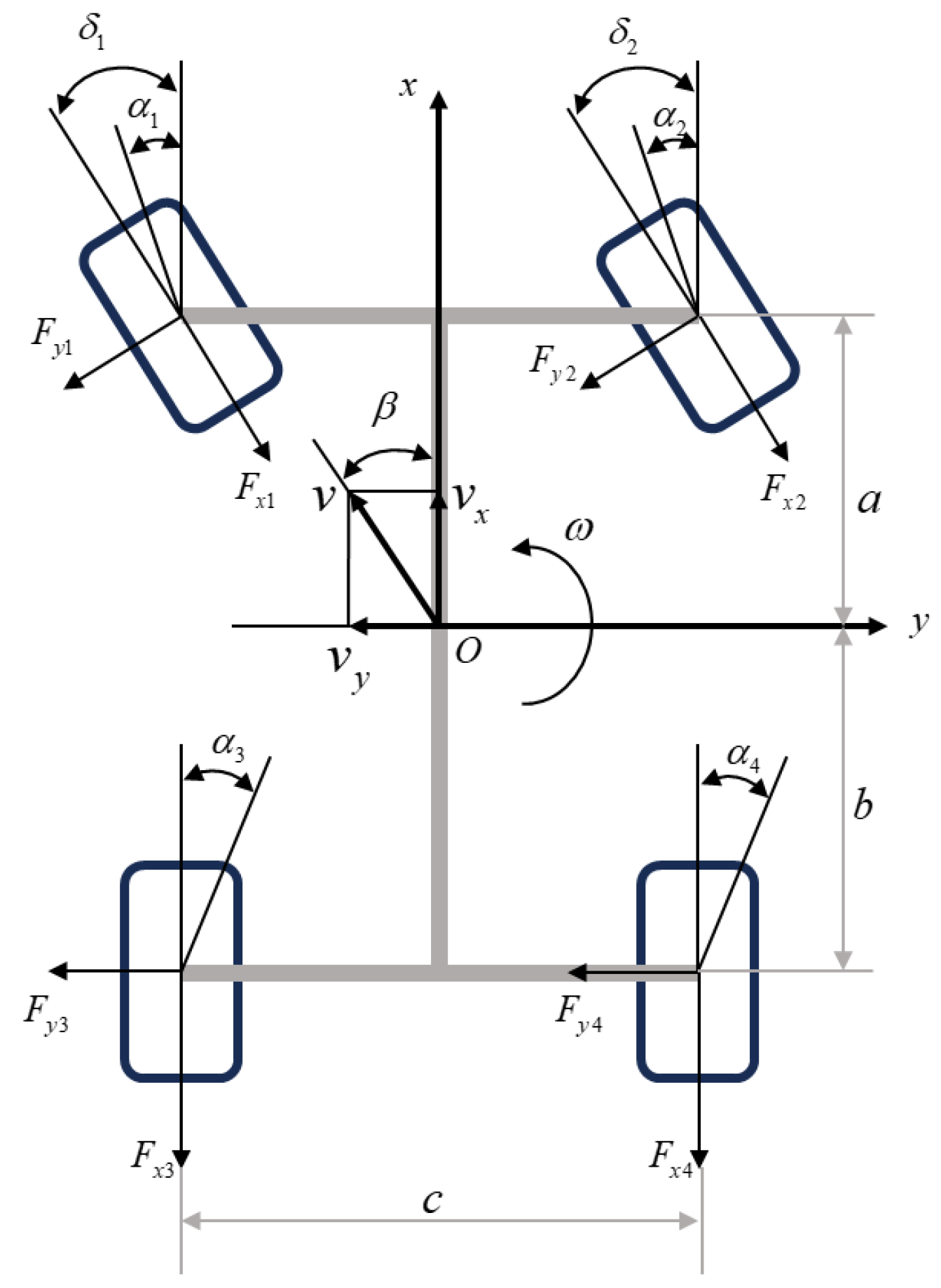
Given that the vertical load, lateral force, and longitudinal force on the tires all exhibit dynamic variations during braking, a seven-degree-of-freedom (7-DOF) vehicle model was established [16] incorporating longitudinal, lateral, and yaw motion and the rotation of all four wheels. To facilitate the analysis of the forces acting on the vehicle during a single-wheel brake failure, practical factors such as air resistance, tire deformation, and sudden changes in the road friction coefficient were neglected. The established model enables the analysis of vehicle dynamics under such failure conditions, as illustrated in Figure 1.

Establish the dynamic equations for longitudinal, lateral, and yaw motions based on Newton’s laws of motion:

$$\begin{array}{c}m({\dot{v}}_x-\omega v_y)=(F_{x1}+F_{x2})\cos {\delta }_f+\\ (F_{y1}+F_{y2})\sin {\delta }_f+F_{x3}+F_{x4}\end{array}$$

(1)

$$\begin{array}{c}m({\dot{v}}_y+\omega v_x)=(F_{y1}+F_{y2})\cos {\delta }_f-\\ (F_{x1}+F_{x2})\sin {\delta }_f+F_{y3}+F_{y4}\end{array}$$

(2)

$$\begin{array}{c}{M}_z=I_z\dot{\omega }=a(F_{x1}+F_{x2})\sin {\delta }_f-\\ a(F_{y1}+F_{y2})\cos {\delta }_f-b(F_{y3}+F_{y4})+T_f\end{array}$$

(3)

$$\begin{array}{c}{T}_f={\displaystyle \frac{c}{2}}[(F_{x1}-F_{x2})\cos {\delta }_f+\\ (F_{y1}-F_{y2})\sin {\delta }_f+(F_{x3}-F_{x4})]\end{array}$$

(4)

In the equation, $m$ represents the vehicle mass,$v_x$ is the longitudinal velocity of the vehicle,${ v}_y$ is the lateral velocity of the vehicle, ${\delta }_f$ is the front-wheel steering angle, a and b are the distances from the vehicle center of mass to the front and rear axles, respectively, c is the vehicle track width,${ I}_z$ is the vehicle moment of inertia about the z-axis, and $T_f$ is the longitudinal component of the vehicle force acting on the center of mass. Here, $1\sim 4$ represent the left front wheel, right front wheel, left rear wheel, and right rear wheel, respectively.${ F}_x$ represents the longitudinal tire force, and $F_y$ represents the lateral tire force.

2.2. Two-Degree-of-Freedom Model

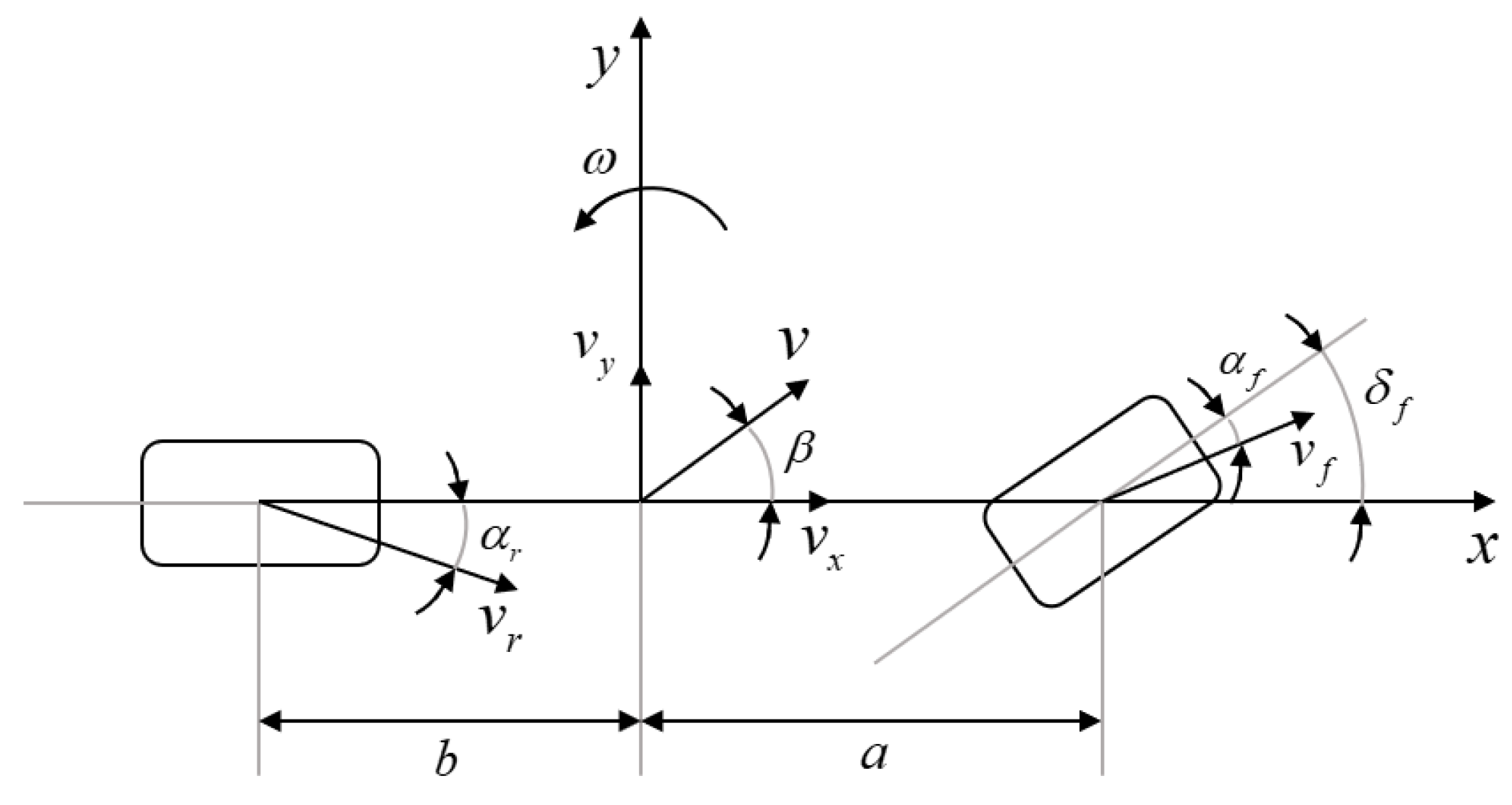
Vehicle stability control relies on precise vehicle dynamics models. This paper employs the two-degree-of-freedom vehicle model shown in Figure 2 as the reference model [17].

$$\left\{\begin{array}{l}\dot{\beta }={\displaystyle \frac{K_f+K_r}{m{v}_x}}\beta +({\displaystyle \frac{a{K}_f-b{K}_r}{m{v}_x^2}}-1)\omega -{\displaystyle \frac{K_f}{m{v}_x}}{\delta }_f\\ \dot{\omega }={\displaystyle \frac{a{K}_f-b{K}_r}{I_z}}\beta +{\displaystyle \frac{a^2{K}_f+b^2{K}_r}{I_z{v}_x}}\omega -{\displaystyle \frac{a{K}_f}{I_z}}{\delta }_f\end{array}\right.$$

(5)

In Equation (5), $K_f,K_r$ represent the lateral stiffness of the front and rear axles, respectively.$\beta$ is the vehicle’s sideslip angle.$\omega$ is the vehicle’s yaw rate.

2.3. Tire Model

The forces and torques generated by tires, such as braking force, lateral force, rolling resistance and self-aligning torque, are key factors influencing vehicle dynamics. To comprehensively describe the longitudinal and lateral forces of a tire, the “Magic Formula” [18] can be used. This formula is less prone to divergence under critical operating conditions such as high slip, varying loads, and high lateral slip, making it suitable for analyzing stability-limited scenarios including wheel lockup, single-wheel failure, and yaw instability [19]:

$$F_{xi}=D_x\sin \{C_x\arctan [B_x{\lambda }_i-E_x(B_x{\lambda }_i-\arctan (B_x{\lambda }_i))]\}$$

(6)

$$F_{yi}=D_y\sin \{C_y\arctan [B_y{\alpha }_i-E_x(B_y{\alpha }_i-\arctan (B_y{\alpha }_i))]\}$$

(7)

In Equations (6) and (7), B, C, D, and E represent tire parameters; ${\lambda }_i$ represents the tire slip ratio; ${\alpha }_i$ represents the tire yaw angle.

In the equation:

$$\left\{\begin{array}{l}{C}_x=b_0\\ D_x=b_1{F}_z^2+b_2{F}_z\\ B_x={\displaystyle \frac{(b_3{F}_z^2+b_4{F}_z)}{C_x{D}_x\exp (b_5{F}_z)}}\\ E_x=b_6{F}_z^2+b_2{F}_z+b_8\end{array}\right.$$

(8)

$$\left\{\begin{array}{l}{C}_y=a_0\\ D_y=a_1{F}_z^2+a_2{F}_z\\ B_y={\displaystyle \frac{a_3\sin (2\arctan (F_z/a_4))(1-a_5\left|\lambda \right|)}{C_x{D}_x}}\\ E_y=a_6{F}_z^2+a_7\end{array}\right.$$

(9)

The various fitting parameters of the tire model under conditions of pure slip and pure lateral offset are shown in

Table 1. Tire model fitting parameters.

$\mathit{i}$	0	1	2	3	4	5	6	7	8
$a_i$	1.65	−21.3	1144	49.6	226	0.069	−0.006	0.056	0.486
$b_i$	1.30	−22.1	1011	1078	1.82	0.208	0.000	−0.354	0.707

.

$$\left\{\begin{array}{l}{F}_{z1}={\displaystyle \frac{mgb}{2\left(a+b\right)}}-{\displaystyle \frac{m{h}_g{a}_x}{2\left(a+b\right)}}-{\displaystyle \frac{m{h}_g{a}_{y}b}{cL}}\\ F_{z2}={\displaystyle \frac{mgb}{2\left(a+b\right)}}-{\displaystyle \frac{m{h}_g{a}_x}{2\left(a+b\right)}}+{\displaystyle \frac{m{h}_g{a}_{y}b}{cL}}\\ F_{z3}={\displaystyle \frac{mg}{2\left(a+b\right)}}+{\displaystyle \frac{m{h}_g{a}_x}{2\left(a+b\right)}}-{\displaystyle \frac{m{h}_g{a}_{y}b}{cL}}\\ F_{z4}={\displaystyle \frac{mga}{2\left(a+b\right)}}+{\displaystyle \frac{m{h}_g{a}_x}{2\left(a+b\right)}}+{\displaystyle \frac{m{h}_g{a}_{y}b}{cL}}\end{array}\right.$$

(10)

In Equation (10), $a_x$ denotes the acceleration of the vehicle in the x-direction; $a_y$ denotes the acceleration of the vehicle in the y-direction; $F_{zi}$ is the vertical load on wheel i.

During vehicle braking instability, the maximum braking force each wheel can generate is related to its vertical load. The vertical load on the tires varies dynamically due to changes in longitudinal and lateral acceleration.

3. The Influence of Braking Intensity on Vehicle Stability

During vehicle motion, a single-wheel brake failure represents the most likely failure scenario. To investigate how front-wheel and rear-wheel brake failures differ in their effects on vehicle stability, this section analyzes the failures of the left front brake system and the right rear brakes as case studies.

3.1. Analysis of Vehicle Stability During Left Front Brake Failure

3.1.1. Theoretical Analysis of Vehicle Stability in the Event of Left Front Brake Failure

$$\left\{\begin{array}{l}{M}_{zx}=(F_{x3}-F_{x2}-F_{x4})c/2\\ M_{zy}=(F_{y2}+F_{y1})a-(F_{y4}+F_{y3})b\\ M_z=M_{zx}+M_{zy}\end{array}\right.$$

(11)

When the braking system of the left front wheel fails, the braking pressure on that wheel is generally considered to be zero, leaving the other three wheels to primarily provide braking force. As shown in Equation (11), the braking force on the left side of the vehicle is significantly less than that on the right side. Due to this imbalance in braking force between the left and right sides, a clockwise yaw moment $M_{zx}$ is generated, causing the vehicle to veer. Meanwhile, according to the theory of the Kamm circle theory, because the braking force on the left front wheel is assumed to be zero, its longitudinal tire utilization decreases, allowing it to generate a greater lateral force. Under extreme conditions, the differing lateral forces exerted by the front and rear axles can also create an additional yaw moment $M_{zy}$, further exacerbating the vehicle’s yaw motion and compromising its lateral stability.

3.1.2. Simulation and Validation of Vehicle Stability with Left Front Brake Failure

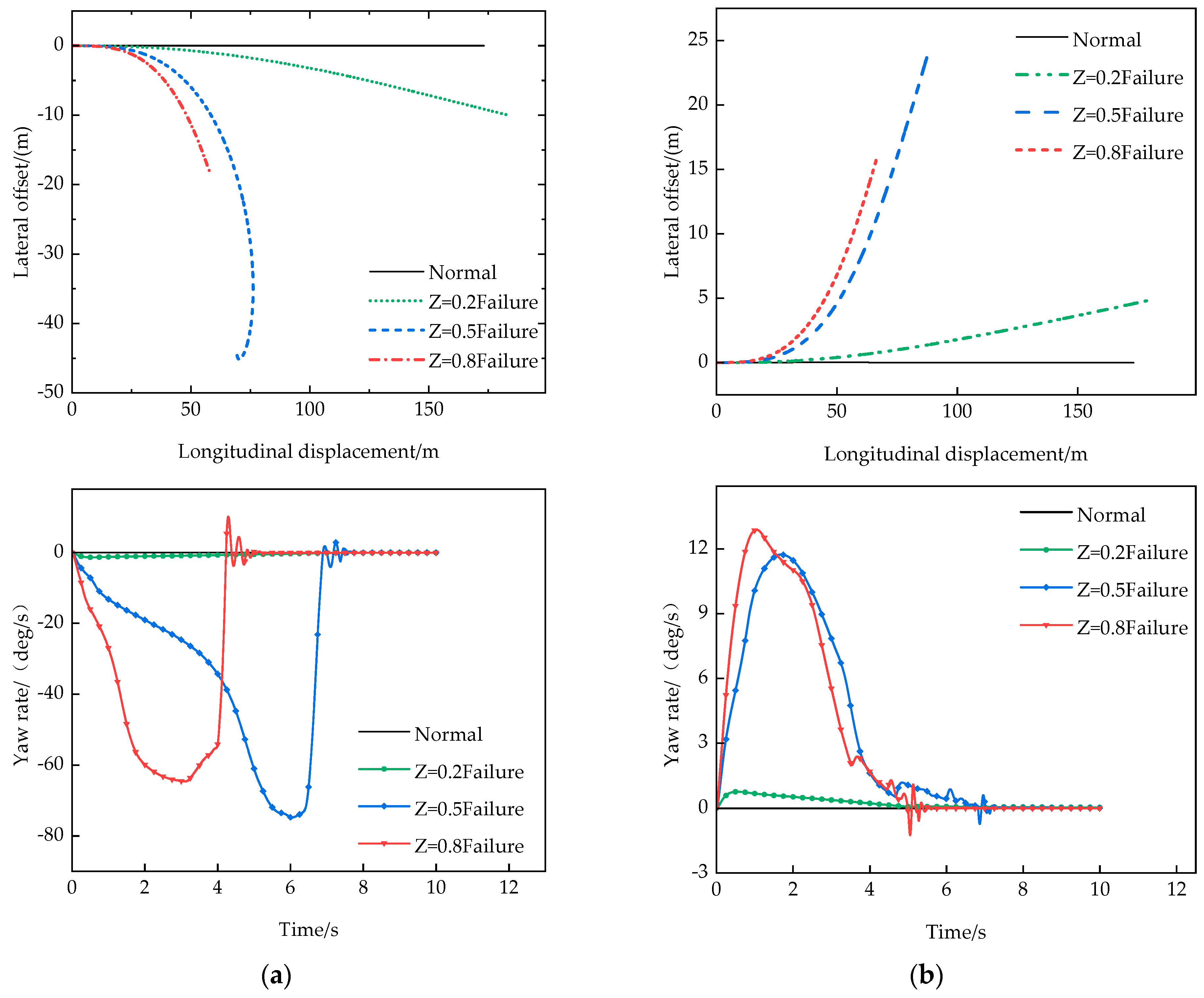
To visually demonstrate the effect of braking force on vehicle stability during a single-wheel brake failure, steering control is temporarily excluded. In this section, we analyze the system using a Simulink–CarSim co-simulation, with a B-Class vehicle in CarSim serving as the reference vehicle. The simulation conditions are set as follows: an initial vehicle speed of V = 100 km/h, braking intensities of $Z=0.5$, road friction coefficients of 0.5 and 0.8, and scenarios involving brake failure on the left front and right rear wheels.

As shown in Figure 3a, due to the failure of the vehicle’s left front brake, the vehicle exhibits a certain degree of lateral offset and an increase in yaw rate under all three braking conditions, indicating relatively poor lateral stability. Specifically, when $Z=0.2$, the vehicle requires a lower braking force, resulting in a relatively small loss of braking force; consequently, the lateral offset and yaw rate remain minimal. However, as the braking intensity increases, the braking force deficit at the failed wheel progressively increases, causing the vehicle’s lateral offset and yaw rate to rise sharply.

In particular, at $Z=0.8$, the maximum lateral offset and yaw rate reached 17.97 m and −64.64$°/\mathrm{s}$, respectively. Under the same longitudinal displacement, compared with Z = 0.2 and Z = 0.5, the lateral offset increased by a factor of 18.5 and 1.88, respectively, while the yaw rate increased by a factor of 79.8 and 2.52, respectively. Consequently, the vehicle’s lateral stability deteriorated significantly, indicating that the impact of a single-wheel brake failure is more severe during high-intensity braking.

3.2. Analysis of Vehicle Stability in the Event of Right Rear Brake Failure

3.2.1. Theoretical Analysis of Vehicle Stability in the Event of Right Rear Brake Failure

$$\left\{\begin{array}{l}{M}_{zx}=(F_{x1}+F_{x3}-F_{x2})c/2\\ M_{zy}=(F_{y2}+F_{y1})a-(F_{y4}+F_{y3})b\\ M_z=M_{zx}+M_{zy}\end{array}\right.$$

(12)

When the braking system of the right rear wheel fails, the braking pressure on that wheel is generally considered to be zero, leaving the other three wheels to primarily provide braking force. At this point, the braking force on the right side of the vehicle is less than that on the left. Due to this imbalance in braking forces, as shown in Equation (12), a counterclockwise moment $M_{zx}$ is generated, causing the vehicle to yaw. Meanwhile, since the braking force on the right rear wheel is assumed to be zero, its longitudinal tire utilization decreases, thereby increasing the available lateral force it can provide. Under extreme conditions, the lateral forces provided by the front and rear axles differ, which also generates a yaw moment $M_{zy}$, further exacerbating the vehicle’s yaw motion and compromising its lateral stability.

3.2.2. Simulation of Vehicle Stability with Right Rear Brake Failure

As shown in Figure 3b, compared with a failure in the left front brake system, a failure in the right rear brake system results in a smaller loss of overall braking force, because less braking force is allocated to the rear wheels during braking. Consequently, the resulting lateral offset and yaw rate tends to correspondingly smaller. However, as the braking intensity gradually increases, the loss of braking force at the right rear wheel becomes more significant, and the vehicle’s stability tends to deteriorate noticeably.

4. Brake Stability Control Strategy

4.1. Brake Force Identification Based on BP Neural Networks

Compared with traditional hydraulic braking systems, in which the brake pedal is mechanically coupled to the brake actuators, the EMB system achieves physical decoupling between the brake pedal and the wheel actuators. This system requires real-time recognition of the driver’s braking intent to precisely regulate clamping force at each wheel through electromechanical actuators. Within the vehicle stability control strategy described herein, the braking intensity Z plays a critical role in clamping force distribution and is therefore of particular importance.

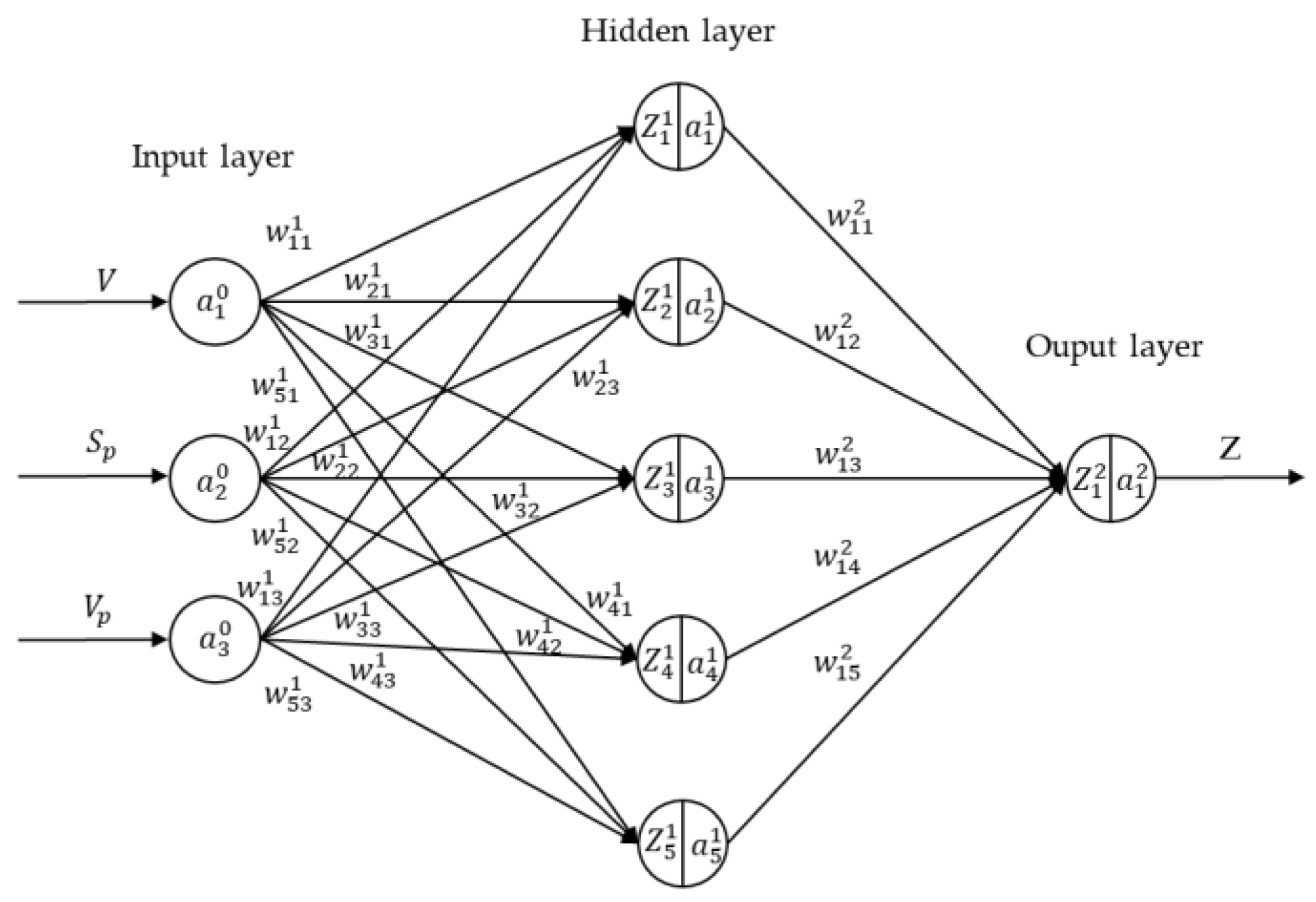
There exists a strong nonlinear mapping relationship between braking intent and driver input, making it difficult to establish an accurate mathematical model for direct representation. As a typical type of multilayer feedforward network, BP neural networks have become the most widely applied neural network architecture in this field due to their global approximation capability for arbitrary nonlinear functions and excellent generalization performance [20,21]. They have been successfully applied for recognizing vehicle driving intentions (such as lane changes and braking scenarios). This paper employs a three-layer BP network architecture (consisting of an input layer, a hidden layer, and an output layer), as shown in Figure 4. Vehicle speed, brake pedal displacement, and the pedal’s rate of change are used as input features, with the output layer mapped to the braking intensity Z [22].

• Principles of BP Neural Networks:

Definition: Input layer: $a_1^0=V, a_2^0=S_p, a_3^0=V_p$; the number of neurons in the hidden layer: M = 5; The number of output layer neurons: $L=1$. Weights and biases: $w_{jk}^l$ denotes the connection from the kth neuron in layer $L-1$ to the jth neuron. It is also the element in the kth column of the jth row of the $l$th-layer weight matrix. Similarly, $b_j^l$ denotes the bias of the jth neuron in layer $l$, which is also the jth element of the bias vector for layer $l$. Let $Z_j^l$ denote the linear output of the jth neuron in the lth layer, and let $a_j^l$ denote the output of the activation function of the jth neuron in the lth layer. In this context, the activation function is denoted by the symbol $\sigma$, and the activation of the jth neuron in the lth layer is as follows:

$$a_j^l=\sigma \left(Z_j^l\right)=\sigma (\sum _k{w}_{jk}^l{a}_k^{l-1}+b_j^l)$$

(13)

$$Z^1=w^1·a^1+b^1=\left[\begin{array}{c}{w}_{11}^1{a}_1^0+w_{12}^1{a}_2^0+w_{13}^1{a}_3^0+b_1^1\\ w_{21}^1{a}_1^0+w_{22}^1{a}_2^0+w_{23}^1{a}_3^0+b_2^1\\ \begin{array}{c}{w}_{31}^1{a}_1^0+w_{32}^1{a}_2^0+w_{33}^1{a}_3^0+b_3^1\\ \begin{array}{c}{w}_{41}^1{a}_1^0+w_{42}^1{a}_2^0+w_{43}^1{a}_3^0+b_4^1\\ w_{51}^1{a}_1^0+w_{52}^1{a}_2^0+w_{53}^1{a}_3^0+b_5^1\end{array}\end{array}\end{array}\right]$$

(14)

$$Z^2=w_{11}^2{a}_1^1+w_{12}^2{a}_2^1+w_{13}^2{a}_3^1{+w}_{14}^2{a}_4^1+w_{15}^2{a}_5^1+b_1^2$$

(15)

The forward propagation process can be expressed as follows:

$$a^l=\sigma (w^l{a}^{l-1}+b^l)$$

(16)

Loss function: To measure the difference between the predicted value $\widehat{Z}$ and the actual value $Z_{true}$, the commonly used mean squared error is employed.

$$L=Loss\left(\widehat{Z}{,Z}_{true}\right)={\displaystyle \frac{1}{2}}{\left(\widehat{Z}{-Z}_{true}\right)}^2$$

(17)

Backpropagation:

Output error:

$${\delta }_j^l={\displaystyle \frac{\partial L}{\partial a_j^l}}{\sigma }^{\prime }\left(Z_j^l\right)$$

(18)

Hidden layer error:

$${\delta }_j^l={\sum }_k{w}_{kj}^{l+1}{\delta }_k^{l+1}{\sigma }^{\prime }\left(Z_j^l\right)$$

(19)

Rate of change of parameters:

$${\displaystyle \frac{\partial L}{\partial b_j^l}}={\delta }_j^l,{\displaystyle \frac{\partial L}{\partial w_{jk}^l}}=a_k^{l-1}{\delta }_j^l$$

(20)

Parameter updates:

$$b_j^l\leftarrow b_j^l-\eta {\displaystyle \frac{\partial L}{\partial b_j^l}},w_{jk}^l\leftarrow w_{jk}^l-\eta {\displaystyle \frac{\partial L}{\partial w_{jk}^l}}$$

(21)

For detailed parameter settings, see Appendix A,

Table A1. BP parameter settings.

Item	Value
Number of input layers	3
Number of output layers	$1$
Number of hidden layers	$5$
Hidden layer activation function	tanh(x)
Output layer activation function	Leaky-ReLU
Learning rate	$0.001$
Optimizer	$Adam$
Loss function	MSE
Mini-batch size	64
Max episodes	1000
Preprocessing method	Normalization

.

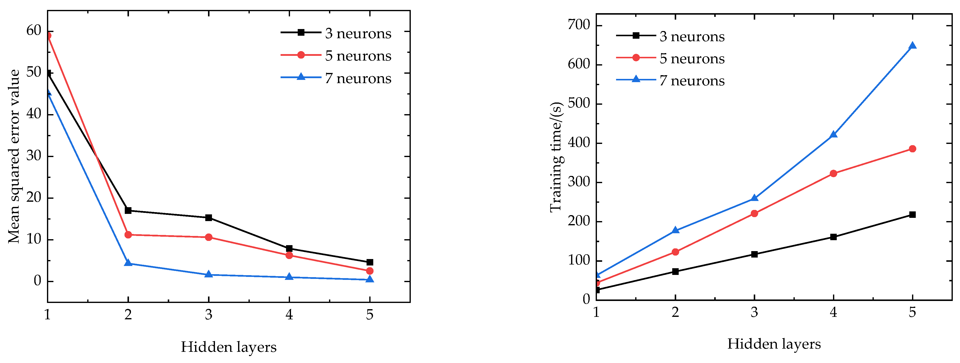
During the braking intensity recognition process, braking intensity simulation parameters exported from CarSim were used to construct the BP neural network model. Specifically, 70% of the data were used to train the neural network, 15% were used as the validation set, and the remaining 15% for testing. When determining the number of hidden layer neurons, both model recognition accuracy and computational speed were taken into account. Based on the evaluation of accuracy and training time across different neuron configurations (as shown in Figure 5), the number of hidden layer neurons was set to 5, with the maximum number of iterations capped at 1000. To prevent overfitting, an early stopping mechanism was employed, which halted the training process when the validation loss ceased to decrease.

To ensure the generalization, approximation capability, and convergence speed of the neural network, the tanh(x) activation function was selected for the hidden layer, and weights were initialized using the Xavier initialization method. Similarly, the Leaky-ReLU activation function was selected for the output layer, and the weights were initialized using the He initialization method.

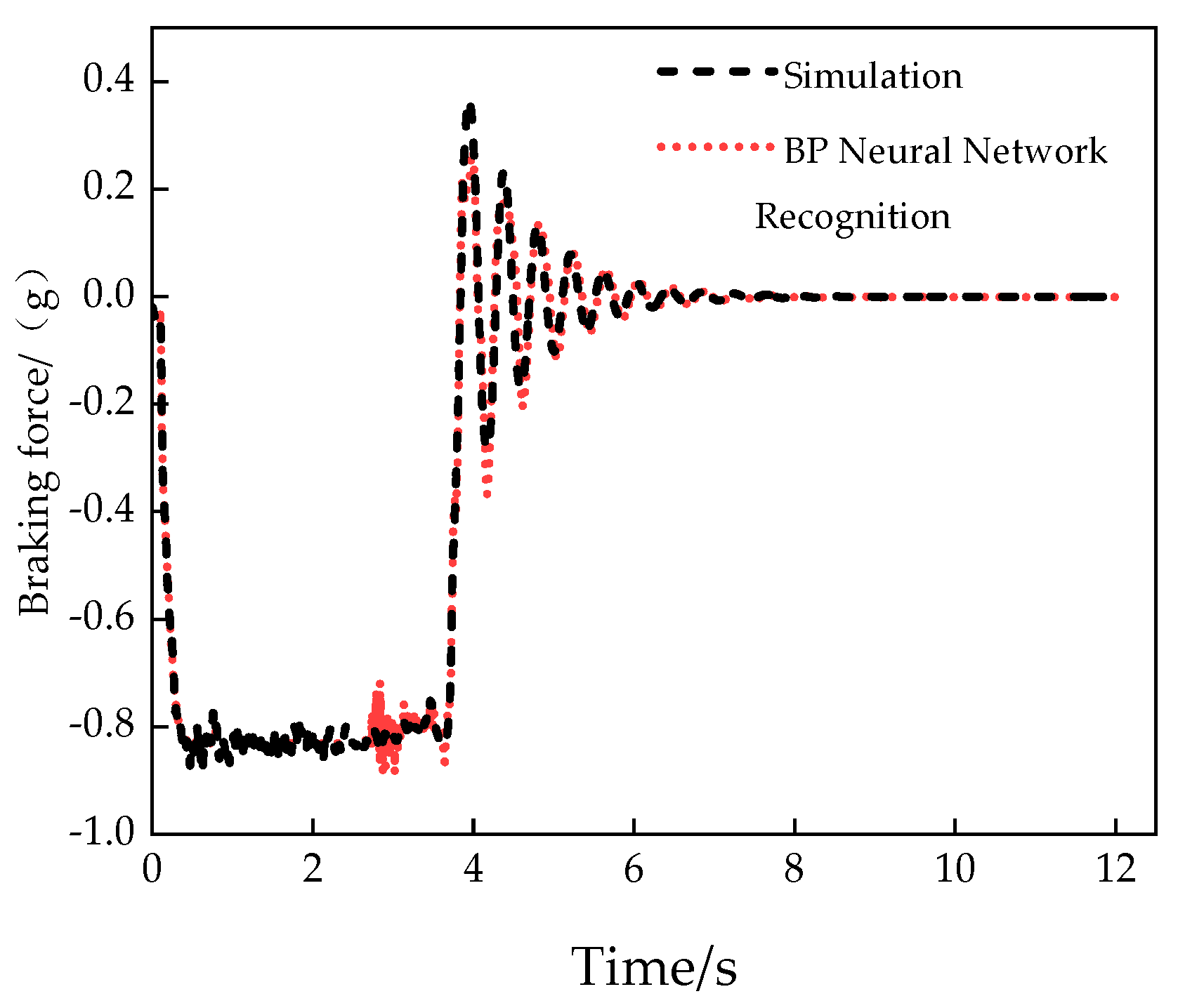
Unseen samples were selected to test the predictive accuracy of the BP neural network. During the braking process, the vehicle gradually decelerated from a maximum speed of 100 km/h until coming to a complete stop. To simulate driver braking behavior, a step-input braking maneuver was employed, in which the brake pedal force rapidly increased to 100 N within 1 s and then remained constant. The model recognition accuracy is shown in Figure 6. The overall prediction error is less than 5%, meeting the accuracy requirements.

4.2. Upper-Level Additional Yaw Moment Control

When implementing vehicle stability control, the vehicle’s sideslip angle and yaw rate are used as reference targets. Therefore, a two-degree-of-freedom dynamic model involving lateral and yaw motions is established, with the yaw moment $∆M$ included, as shown in the following equation:

$$\left\{\begin{array}{l}\dot{\beta }={\displaystyle \frac{K_f+K_r}{m{v}_x}}\beta +({\displaystyle \frac{a{K}_f-b{K}_r}{m{v}_x^2}}-1)\omega -{\displaystyle \frac{K_f}{m{v}_x}}{\delta }_f\\ \dot{\omega }={\displaystyle \frac{a{K}_f-b{K}_r}{I_z}}\beta +{\displaystyle \frac{a^2{K}_f+b^2{K}_r}{I_z{v}_x}}\omega -{\displaystyle \frac{a{K}_f}{I_z}}{\delta }_f+{\displaystyle \frac{\Delta M}{I_z}}\end{array}\right.$$

(22)

When the vehicle is traveling steadily, i.e., $\dot{\beta }=0$ and $\dot{\omega }=0$, the expected sideslip angle ${\beta }_d$ and expected yaw rate ${\omega }_d$ can be obtained from the above equation:

$${\beta }_d=({\displaystyle \frac{b}{L{v}_x}}+{\displaystyle \frac{ma}{L{K}_r}}{v}_x){\omega }_d$$

(23)

$${\omega }_d={\displaystyle \frac{v_x}{(1+K{v}_x^2)L}}{\delta }_f$$

(24)

$$K={\displaystyle \frac{m}{L^2}}({\displaystyle \frac{a}{K_r}}-{\displaystyle \frac{b}{K_f}})$$

(25)

where $K$ is the stability coefficient.

Taking into account the constraints imposed by the road surface coefficient of friction $\mu$, the modified expected sideslip angle and yaw rate are obtained as follows:

$${\beta }_{ref}=\min \left\{\left|{\beta }_d\right|,\left|\mu g({\displaystyle \frac{b}{v_x^2}}+{\displaystyle \frac{ma}{K_f(a+b)}})\right|\right\}\mathrm{sgn}({\delta }_f)$$

(26)

$${\omega }_{ref}=\min \left\{\left|{\omega }_d\right|,\left|{\displaystyle \frac{\mu g}{v_x}}\right|\right\}\mathrm{sgn}({\delta }_f)$$

(27)

In the calculation of yaw moments in the upper-layer controller, PID control, MPC and SMC are commonly used. PID control relies heavily on empirical tuning, while MPC, although more accurate, involves a significant computational burden, which can affect the system’s real-time performance [23,24,25]. Therefore, SMC was selected as the method for calculating the vehicle’s additional yaw moment.

Based on the nonlinear characteristics of the vehicle dynamics model, SMC is employed to calculate the yaw moment to be applied to the vehicle [26,27,28]. To eliminate the chattering phenomenon during the switching process of SMC, an adaptive gain dynamic weighting reaching law is introduced in this paper [29].

Define the sliding surface as follows:

$$s=c_1{e}_{\beta }+c_2{e}_{\omega }+{\displaystyle \int \left(k_{\beta }{e}_{\beta }+k_{\omega }{e}_{\omega }\right)}d\tau$$

(28)

In Formula (28), $e_{\beta }=\beta -{\beta }_d$, $e_{\omega }=\omega -{\omega }_d$, $c_1>0$, $c_2>0$, $k_{\beta }>0$, and $k_{\omega }>0$.

The law of convergence is as follows:

$$\dot{s}=-k(s)·\varphi \left(s\right)$$

(29)

$$\varphi \left(s\right)=\left[\left(1-\sigma \left(s\right)\right)\tanh \left({\displaystyle \frac{s}{{\epsilon }_1}}\right)+\sigma \left(s\right){\displaystyle \frac{s}{{\epsilon }_2+\left|s\right|}}\right]$$

(30)

In Equation (29), the adaptive gain term is as follows:

$$k\left(s\right)=k_0+k_1{\left(\left|s\right|+\epsilon \right)}^{k\left|s\right|-1}+k_2{\displaystyle \frac{\left|s\right|}{a+\left|s\right|}}$$

(31)

$k,{ k}_0,{ k}_1, k_2, \epsilon ,{ \epsilon }_1, {\epsilon }_2, a$ represent positive constants, where $k_0$ is the base gain used to overcome inherent system uncertainties and disturbances, and $k_1{(\left|s\right|+\epsilon )}^{k\left|s\right|-1}$ is the exponential adaptive term that provides nonlinear gain adjustment. When the system’s state deviates significantly from the sliding surface, the gain increases rapidly to accelerate convergence. As the system approaches the sliding surface, the gain decreases to suppress chattering. $k_2(\left|s\right|/(a+\left|s\right|\left)\right)$ is the saturation adaptive term, which accelerates convergence when the system is far from the equilibrium point and decelerates convergence near the equilibrium point to suppress chattering.

In Equation (30), $\sigma \left(s\right)$ represents the dynamic weighting factor:

$$\sigma \left(s\right)={\displaystyle \frac{1}{1+\exp \left(-\alpha \left(\left|s\right|-\rho \right)\right)}}·e^{-\xi t}$$

(32)

where $\alpha$, $\rho$ and $\xi$ are positive constants, and $1/\left[1+\mathrm{e}\mathrm{x}\mathrm{p}(-\mathsf{\alpha }(\left|s\right|-\rho \left)\right)\right]$ represents the error-driving term. When $\left|s\right|\gg \rho$, this term approaches 1, enabling rapid system convergence. When $\left|s\right|\ll \rho$, this term approaches 0, suppressing system chattering. The term $e^{-\xi t}$ denotes the time decay term, which gradually attenuates over time to enable a smoothing mode.

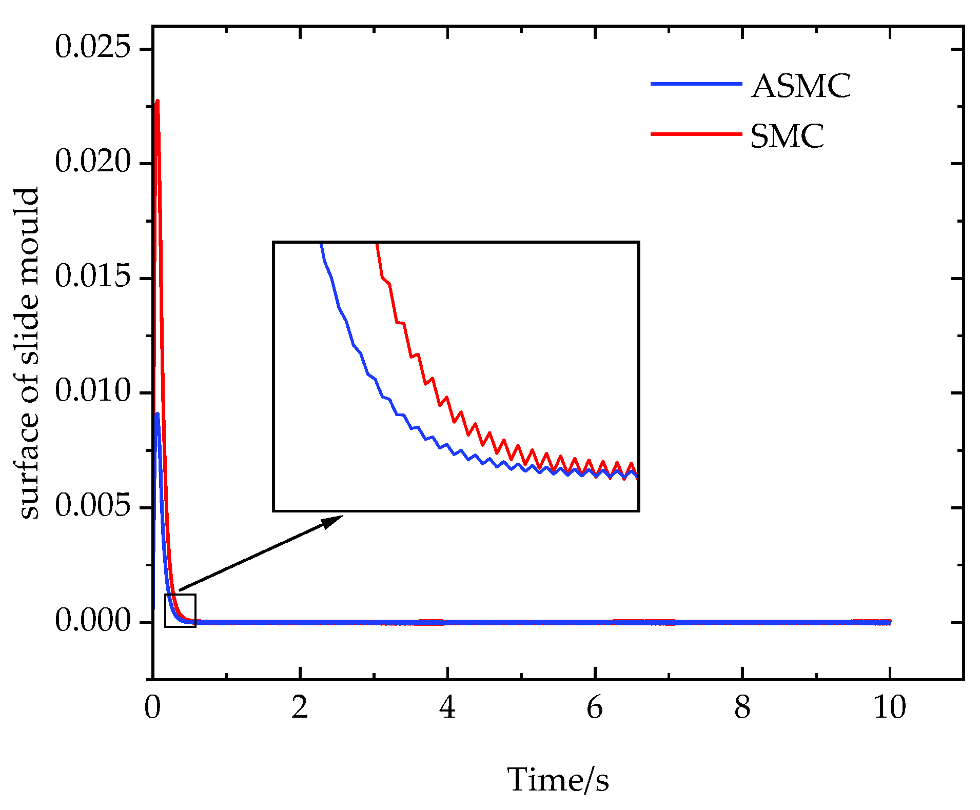
As shown in Figure 7, compared with traditional exponential convergence algorithms, the adaptive reaching law proposed in this paper exhibits a faster convergence rate and shorter dynamic response time. Furthermore, the chattering phenomenon is significantly suppressed, indicating that this method can effectively improve transient performance and enhance control smoothness.

(1)

Proof of stability:

Select the Lyapunov function:

$$V_1={\displaystyle \frac{1}{2}}{s}^2$$

(33)

$$\begin{array}{cc}\hfill {\dot{V}}_1& =s\dot{s}\hfill \\ \hfill & =-k\left(s\right)·s·\varphi \left(s\right)\hfill \end{array}$$

(34)

According to the Lyapunov stability criterion, if $\dot{V}\le 0$, the system is stable. From Equation (32), we know that $0<\sigma \left(s\right)<1$. When $s>0$, $\varphi \left(s\right)>0$, and when $s<0$, $\varphi \left(s\right)<0$; therefore, $s·\varphi \left(s\right)>0$. Furthermore, from Equation (31), we know that k(s) > 0; thus, the following equation holds true:

$$\begin{array}{cc}\hfill {\dot{V}}_1& =s\dot{s}\hfill \\ \hfill & =-k\left(s\right)·s·\varphi \left(s\right)\le 0\hfill \end{array}$$

(35)

Therefore, based on the Lyapunov stability criterion, the system is stable.

The desired yaw moment $M_z$ is obtained by combining Equations (22), (28) and (29).

$$\begin{array}{l}\Delta M=I_z\left[{\displaystyle \frac{-k\left(s\right)·\varphi \left(s\right)-c_1{\dot{e}}_{\beta }-k_{\beta }{e}_{\beta }-k_{\omega }{e}_{\omega }}{c_2}}\right.+{\dot{\omega }}_d\\ \begin{array}{cc}& \end{array}\left.-\left({\displaystyle \frac{a{k}_f-b{k}_r}{I_z}}\beta +{\displaystyle \frac{a^2{k}_f+b^2{k}_r}{I_z{v}_x}}\omega -{\displaystyle \frac{a{k}_f}{I_z}}{\delta }_f\right)\right]\end{array}$$

(36)

Define the system tracking error state vector as $e\left(t\right)={\left[\begin{array}{cc}{e}_{\beta }\left(t\right)& e_{\omega }\left(t\right)\end{array}\right]}^T$, where $e_{\beta }=\beta -{\beta }_d$ and $e_{\omega }=\omega -{\omega }_d$. Combining this with Equation (22), the open-loop error dynamics equation including disturbances can be expressed as follows:

$$\left\{\begin{array}{c}{\dot{e}}_{\beta }=f_{\beta }\left(\beta ,\omega ,{\delta }_f\right)-{\dot{\beta }}_d+d_{\beta }\left(t\right)\\ {\dot{e}}_{\omega }=f_{\omega }\left(\beta ,\omega ,{\delta }_f\right)-{\dot{\omega }}_d+{\displaystyle \frac{∆M}{I_z}}+d_{\omega }\left(t\right)\end{array}\right.$$

(37)

Taking the derivative of Equation (28) yields the following:

$$\dot{s}=c_1{\dot{e}}_{\beta }+c_2{\dot{e}}_{\omega }+k_{\beta }{e}_{\beta }+k_{\omega }{e}_{\omega }$$

(38)

Substitute Equation (36) into Equation (37):

$${\dot{e}}_{\omega }=f_{\omega }-{\dot{\omega }}_d+\left[{\displaystyle \frac{-k\left(s\right)\varphi \left(s\right)-c_1{\dot{e}}_{\beta }-k_{\beta }{e}_{\beta }-k_{\omega }{e}_{\omega }}{c_2}}+{\dot{\omega }}_d-f_{\omega }\right]+d_{\omega }\left(t\right)$$

(39)

This can be simplified to the following:

$${\dot{e}}_{\omega }=-{\displaystyle \frac{c_1}{c_2}}{\dot{e}}_{\beta }-{\displaystyle \frac{k_{\beta }}{c_2}}{e}_{\beta }-{\displaystyle \frac{k_{\omega }}{c_2}}{e}_{\omega }-{\displaystyle \frac{k\left(s\right)}{c_2}}\varphi \left(s\right)+d_{\omega }\left(t\right)$$

(40)

This yields the following complete closed-loop error dynamics matrix equation:

$$\left[\begin{array}{c}{\dot{e}}_{\beta }\\ {\dot{e}}_{\omega }\end{array}\right]=A_c\left[\begin{array}{c}{e}_{\beta }\\ e_{\omega }\end{array}\right]+\left[\begin{array}{c}0\\ -{\displaystyle \frac{k\left(s\right)}{c_2}}\varphi \left(s\right)\end{array}\right]+\left[\begin{array}{c}{d}_{\beta }\left(t\right)\\ d_{\omega }\left(t\right)-{\displaystyle \frac{c_1}{c_2}}{d}_{\beta }\left(t\right)\end{array}\right]$$

(41)

where $A_c$=$\left[\begin{array}{cc}{A}_{11}& A_{12}\\ A_{21}& A_{22}\end{array}\right]$, $A_{11}={\displaystyle \frac{K_f+K_r}{m{v}_x}}$, $A_{12}={\displaystyle \frac{a{K}_f-b{K}_r}{m{v}_x^2}}-1$, $A_{21}=\left[-{\displaystyle \frac{1}{c_2}}\left(c_1{\displaystyle \frac{K_f+K_r}{m{v}_x}}+k_{\beta }\right)\right]$, and $A_{22}=\left[-{\displaystyle \frac{1}{c_2}}\left(c_1\left({\displaystyle \frac{a{K}_f-b{K}_r}{m{v}_x^2}}-1\right)+k_{\omega }\right)\right]$

(2)

Proof of Accessibility:

In real-world physical systems, two-degree-of-freedom vehicle models must account for external disturbances and parameter uncertainties. Let the derivative of the actual sliding surface be

$$\dot{s}=-k\left(s\right)·\varphi \left(s\right)+d\left(t\right),$$

(42)

where d(t) is the total disturbance term, and $\left|d\left(t\right)\right|\le D$.

Define a minimal sliding mode boundary layer $\mathsf{\Omega }=\left\{s\left|\left|s\right|\le \Delta \right.\right\}$, where $\Delta >0$.

When the system’s state lies outside the boundary, i.e., $\left|s\right|>∆$, due to the properties of the $\mathrm{t}\mathrm{a}\mathrm{n}\mathrm{h}\left(x\right)$ function, there must exist a constant $\delta \in \left(\mathrm{0,1}\right)$ strictly greater than zero such that the following equation holds true:

$$\left|\varphi \left(s\right)\right|\ge \delta , \forall \left|s\right|>∆$$

(43)

Furthermore, as shown above, s and ϕ(s) always have the same sign; therefore, when |s| > ∆, the following holds:

$$s·\varphi \left(s\right)=\left|s\right|\left|\varphi \left(s\right)\right|\ge \delta \left|s\right|$$

(44)

Substitute Equation (42) into Equation (34):

$$\dot{V_1}=s\dot{s}=s\left[-k\left(s\right)·\varphi \left(s\right)+d\left(t\right)\right]$$

(45)

$$\dot{V_1}=-k\left(s\right)·s·\varphi \left(s\right)+s·d\left(t\right)$$

(46)

Substitute the perturbation upper bound $\left|d\left(t\right)\right|\le D$:

$$\dot{V_1}\le -k\left(s\right)·\left|s\right|·\left|\varphi \left(s\right)\right|+\left|s\right|·\left|d\left(t\right)\right|$$

(47)

$$\dot{V_1}\le -k\left(s\right)·\delta ·\left|s\right|·+D·\left|s\right|=-(k\left(s\right)\delta -D)\left|s\right|$$

(48)

From Equation (31), it follows that $k\left(s\right)\ge k_0$; therefore, the basic gain k₀ must satisfy the following condition:

$$k_0\delta -D\ge \eta >0$$

(49)

Let $\eta$ be a positive constant; substituting this into Equation (42) gives the following:

$${\dot{V}}_1\le -\eta \left|s\right|$$

(50)

Since $\left|s\right|=\sqrt{2V_1 }$, the above equation can be rewritten as follows:

$${\dot{V}}_1\le -\eta \sqrt{2V_1}$$

(51)

(3)

Proof of System State Boundedness:

$$\dot{\beta }=A_{11}\beta +A_{12}\omega +B_1{\delta }_f$$

(52)

where $A_{11}={\displaystyle \frac{K_f+K_r}{m{v}_x}}$, $A_{12}={\displaystyle \frac{a{K}_f-b{K}_r}{m{v}_x^2}}-1$, and $B_1=-{\displaystyle \frac{K_f}{m{v}_x}}$.

Substituting the tracking errors $e_{\beta }=\beta -{\beta }_d$ and $e_{\omega }=\omega -{\omega }_d$ yields the following equation:

$${\dot{e}}_{\beta }=A_{11}{e}_{\beta }+A_{12}{e}_{\omega }+D_{\beta }\left(t\right)$$

(53)

where $D_{\beta }\left(t\right)=A_{11}{\beta }_d+A_{12}{\omega }_d+B_1{\delta }_f-{\dot{\beta }}_d$

From Equations (26) and (27), it follows that ${\beta }_d$ and ${\omega }_d$ are strictly constrained by the road surface coefficient of friction $\mu$, and the front-wheel steering angle ${\delta }_f$ is determined by the driver’s physical input; therefore, $D_{\beta }\left(t\right)$ must be bounded (i.e., there exists a constant $D_m>0$ such that $\left|D_{\beta }\left(t\right)\right|\le D_m$).

Compute the time derivative of the designed integral sliding surface (Equation (28)):

$$\dot{s}=c_1{\dot{e}}_{\beta }+c_2{\dot{e}}_{\omega }+k_{\beta }{e}_{\beta }+k_{\omega }{e}_{\omega }$$

(54)

Since $\Delta \mathrm{M}$ appears only in ${\dot{e}}_{\omega }$ as a control input, we rearrange the terms to express the controlled term ${\dot{e}}_{\omega }$ in terms of the uncontrolled term and other bounded variables:

$${\dot{e}}_{\omega }=-{\displaystyle \frac{c_1}{c_2}}{\dot{e}}_{\beta }-{\displaystyle \frac{k_{\beta }}{c_2}}{e}_{\beta }-{\displaystyle \frac{k_{\omega }}{c_2}}{e}_{\omega }+{\displaystyle \frac{1}{c_2}}\dot{s}$$

(55)

Substituting Equation (53) into the above equation yields the following:

$${\dot{e}}_{\omega }=-\left({\displaystyle \frac{c_1{A}_{11}+k_{\beta }}{c_2}}\right)e_{\beta }-\left({\displaystyle \frac{c_1{A}_{12}+k_{\omega }}{c_2}}\right)e_{\omega }-{\displaystyle \frac{c_1}{c_2}}{D}_{\beta }\left(t\right)+{\displaystyle \frac{1}{c_2}}\dot{s}$$

(56)

Combine Equations (48) and (51) and write them in standard state-space matrix form:

$$\left[\begin{array}{c}{\dot{e}}_{\beta }\\ {\dot{e}}_{\omega }\end{array}\right]=\left[\begin{array}{cc}{A}_{11}& A_{12}\\ -{\displaystyle \frac{c_1{A}_{11}+k_{\beta }}{c_2}}& -{\displaystyle \frac{c_1{A}_{12}+k_{\omega }}{c_2}}\end{array}\right]\left[\begin{array}{c}{e}_{\beta }\\ e_{\omega }\end{array}\right]+\left[\begin{array}{cc}1& 0\\ -{\displaystyle \frac{c_1}{c_2}}& {\displaystyle \frac{1}{c_2}}\end{array}\right]\left[\begin{array}{c}{D}_{\beta }\left(t\right)\\ \dot{s}\left(t\right)\end{array}\right]$$

(57)

$${\left[\begin{array}{cc}{\dot{e}}_{\beta }& {\dot{e}}_{\omega }\end{array}\right]}^T=A_{err}{\left[\begin{array}{cc}{e}_{\beta }& e_{\omega }\end{array}\right]}^T+B_{err}{\left[\begin{array}{cc}{D}_{\beta }\left(t\right)& \dot{s}\left(t\right)\end{array}\right]}^T$$

(58)

The above equations constitute a zero-error dynamic model of the system constrained near the sliding surface. During controller parameter design, by appropriately setting the positive constants $c_1$, $c_2$, $c_3$ and $c_4$, the error system matrix $A_{err}$ is ensured to satisfy the Hurwitz stability criterion.

As shown in Equations (33)–(35), the sliding mode variables remain within a finite boundary layer; therefore, the external excitation vector ${\left[\begin{array}{cc}{D}_{\beta }\left(t\right)& \dot{s}\left(t\right)\end{array}\right]}^T$ is strictly bounded. According to the Input-to-State Stability (ISS) theorem in nonlinear control theory, the states of a strictly Hurwitz-stable linear system are necessarily bounded when driven by a bounded external input.

Therefore, the tracking error vector ${\left[\begin{array}{cc}{e}_{\beta }& e_{\omega }\end{array}\right]}^T$ is bounded. Meanwhile, Equations (26) and (27) show that the reference trajectory is bounded by physical constraints. According to the principle of linear superposition for bounded signals, the actual physical state variables—$\beta$ and $\omega$—in the closed-loop system are both bounded. Thus, while ensuring error convergence, this controller fundamentally guarantees the safety and stability of the vehicle’s chassis dynamics.

4.3. Parameter Optimization Based on the TD3 Reinforcement Learning Algorithm

TD3 is a model-free reinforcement learning (RL) method. It learns optimal policies through direct interaction with the environment (input states, output actions/parameters). Consequently, it can learn directly from data how to tune controller parameters for an uncertain or complex system without requiring knowledge of the system’s exact differential equations. This is of significant value for real-world systems where accurate modeling is notoriously challenging.

Addressing the challenges posed by strong nonlinearity, parameter perturbations, and position disturbances in electro-hydraulic servo systems—challenges that traditional control algorithms struggle to resolve—Reference [30] proposed an intelligent composite control strategy that integrates the TD3 deep reinforcement learning algorithm with adaptive fractional-order sliding mode control. A fractional-order sliding surface was designed, along with a reaching law function based on the sliding surface. Adaptive control laws were designed based on Lyapunov stability theory, and the gain parameters for sliding mode switching were optimized online using the TD3 deep reinforcement learning algorithm. Furthermore, in response to the issues of excessive reliance on manual experience, low efficiency, and cumbersome procedures in the selection of PID controller parameters, Reference [31] proposed a PID parameter optimization method based on the TD3 algorithm.

Given that the adaptive variable-gain sliding mode controller design involves numerous parameters, the sliding surface coefficients and controller gains typically rely on prior knowledge of the system’s dynamic model. For complex nonlinear, time-varying, or partially modeled systems, manually or model-based tuning of these parameters is extremely challenging, often requiring a difficult trade-off between robustness and chattering. Relying solely on manual adjustment results in a heavy workload and often leads to suboptimal performance. To address these limitations, this paper incorporates the TD3 algorithm from reinforcement learning to achieve autonomous parameter optimization [32,33].

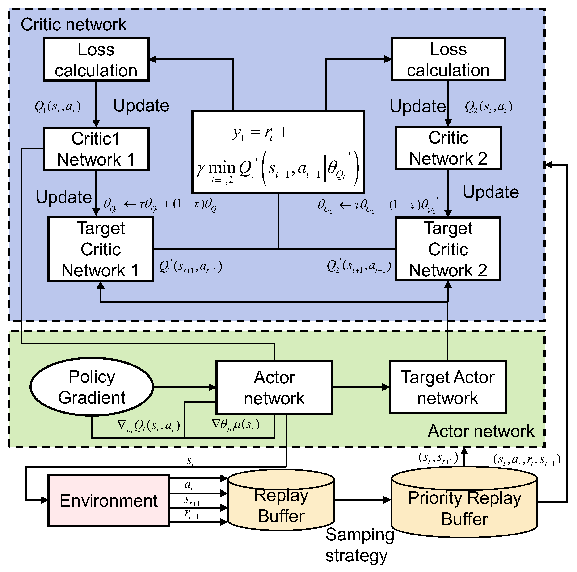
TD3 (Twin Delayed Deep Deterministic Policy Gradient) is an enhanced actor–critic algorithm developed to address the limitations of DDPG. Its three key core mechanisms—twin critics, delayed policy updates, and target policy smoothing—are specifically designed to suppress Q-value overestimation, stabilize the training process, and enhance policy generalization. These mechanisms effectively mitigate common issues encountered in DDPG during continuous control tasks, such as training oscillations, premature convergence to local optima, and potential divergence. The specific implementation details are as follows:

(1)

Twin Critics: Mitigating Overestimation of Q-values at the Source

When DDPG uses a single Q-network, environmental noise, sample bias, and function approximation errors cause the Q-values to systematically overestimate the true action values (i.e., they treat certain actions as better than they actually are). This overestimation is propagated through gradients to the policy network, causing the policy to continuously optimize toward “overestimated bad actions,” ultimately converging to a local optimum or even divergence.

The core principle of TD3 is to simultaneously train two independent value networks (Q₁, Q₂), which share the same policy network but do not interfere with one another; Meanwhile, two target value networks (Q₁′, Q₂′) are also maintained. When calculating the target Q-value, the minimum of the outputs from the two target Q-networks is taken:

$$y_t=r_t+\gamma \underset{i=1,2}{\min }{Q_i}^{\prime }(s_{t+1},a_{t+1}\left|{{\theta }_{Qi}}^{\prime }\right.)$$

(59)

Substitute into the Bellman equation to find the solution function:

$$L({\theta }_{Q_i})={\displaystyle \frac{1}{M}}{\displaystyle {\sum }_{i=1}^M(y_t-Q_i(s_t,a_t\left|{\theta }_{Q_i}\right.))}$$

(60)

Here, M represents the number of action samples in the experience replay buffer, and ${\theta }_{Q_i}$ represents the parameters of the target critic network.

(2)

Delayed update policy:

Unlike the synchronous update mechanism for the policy network and Q-network in DDPG, where even minor fluctuations in Q-values are directly passed to the policy network, causing policy oscillations, the TD3 algorithm innovatively introduces a delayed update strategy. Specifically, the Q-network is updated d times first until it converges sufficiently to a relatively stable state, and only then is the policy network is updated. This approach establishes a more stable mapping from the continuous state space to action values. During the parameter iteration process, the algorithm uses backpropagation to optimize the parameters of the actor network, as mathematically expressed below:

$${\displaystyle \frac{\partial J({\theta }_{\mu })}{\partial {\theta }_{\mu }}}={\displaystyle \frac{1}{M}}{\displaystyle {\sum }_{i=1}^M\left[{\nabla }_a{Q}_i(s_t,a_t|{\theta }_{Q_i}){|}_{a_t=\mu (s_t|{\theta }_{\mu })}\nabla {\theta }_{\mu }\mu (s_t|{\theta }_{\mu })\right]}$$

(61)

In the equation, $\partial J\left({\theta }_{\mu }\right)/\partial \left({\theta }_{\mu }\right)$ represents the loss gradient; $\nabla$ denotes the gradient; ${\theta }_{\mu }$ denotes the parameters of the actor network; and $\mu$ denotes the actor network.

At the same time, the target network has been updated as follows:

$$\left\{\begin{array}{l}{{\theta }_{Qi}}^{\prime }\leftarrow \tau {\theta }_{Q_i}+(1-\tau ){{\theta }_{Qi}}^{\prime }\\ {{\theta }_{\mu }}^{\prime }\leftarrow \tau {\theta }_{\mu }+(1-\tau ){{\theta }_{\mu }}^{\prime }\end{array}\right.$$

(62)

Here, $\tau$ is the soft update parameter, with a value between 0 and 1.

(3)

Optimization of the smoothness of the objective function:

In DDPG, the target policy directly outputs deterministic actions, and the Q-values are highly sensitive to even minor changes in these actions. TD3 smooths the target policy by adding normally distributed noise to the target actions, thereby smoothing the value estimates across the action space and improving the policy’s generalization to environmental disturbances and parameter perturbations, as shown below:

$$\tilde{a}={\mu }^{\prime }(s_{t+1}\left|{{\theta }_{\mu }}^{\prime }\right.)+\epsilon , \epsilon \sim clip(N(0,\sigma ),-c,c),c>0$$

(63)

Here, $\epsilon$ represents random noise following a normal distribution; $\sigma$ represents the variance; and c represents the clipping factor.

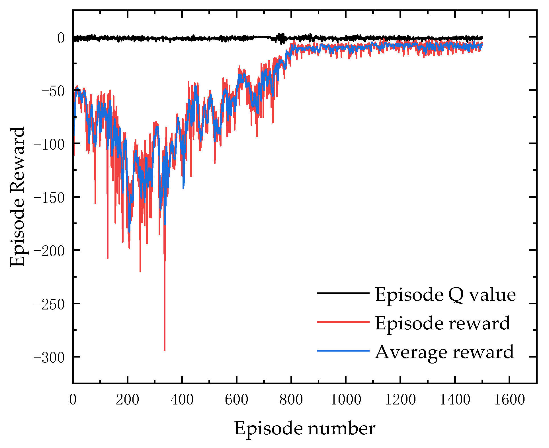
For detailed parameter settings, see Appendix A,

Table A2. TD3 parameter settings.

Hyperparameters
Item	Value
Critic learning rate	$1\times {10}^{-3}$
Actor learning rate	$1\times {10}^{-4}$
Target network update frequency	1
Sample time	0.01
Target smooth factor	$1\times {10}^{-3}$
Experience buffer size	$1\times {10}^6$
Discount factor	0.9
Mini-batch size	64
Max episodes	500

; for the pseudocode of the training process, see Appendix B, Algorithm A1. Figure 8 illustrates the structure of the TD3 algorithm. Figure 9 shows the training curve of the TD3 algorithm.

The intelligent agent module encompasses the primary execution process of the decision-making algorithm, responsible for receiving inputs and making decisions. Input state information includes the sideslip angle $\beta$, yaw rate $\omega$, and lateral offset y, as follows:

$$s_t=\left\{\beta ,\omega ,y\right\}$$

(64)

The action space for the intelligent agent is selected as the sliding surface parameters $C_1$, $C_2$, $k_{\alpha }$, $k_{\beta }$ and the tracking law parameters $k_0$, $k_1$, $k_2$ for the sliding mode controller, expressed as follows:

$$a_t=\left\{C_1,C_2,k_{\alpha },k_{\beta },k_0,k_1,k_2\right\}$$

(65)

The reward function is crucial for optimizing sliding mode control. To enable the agent to achieve multi-objective cooperative optimization, the following objective rewards are designed:

$$r=-w_1{e}_{\beta }-w_2{e}_{\omega }-w_3{e}_y$$

(66)

In the equation, $e_{\beta }$ represents the error between the ideal sideslip angle and the actual sideslip angle; $e_{\omega }$ represents the error between the ideal yaw rate and the actual yaw rate; $e_y$ represents the error between the ideal lateral offset and the actual lateral offset. $w_1$, $w_2$, and $w_3$ are the sideslip angle, yaw rate, and lateral offset, respectively.

4.4. Lower-Level Brake Force Distribution Control

To enhance braking stability following a vehicle braking failure, an objective function is established by comprehensively considering the tire adhesion ellipse [34] and the relationship between lateral force and tire utilization. The optimization objectives aim to maximize the wheel braking force and available lateral force while minimizing the yaw moment. Accordingly, the objective function is formulated as follows:

$$\begin{array}{cc}\min J=& \min \left\{\left[mZg-\left(F_{x1}+F_{x2}\right)\cos {\delta }_f-F_{x3}-F_{x4}\right]\right.\\ & +{\displaystyle \frac{c}{2}}\left[\left(F_{x1}\cos {\delta }_f+F_{x3}\right)-\left(F_{x2}\cos {\delta }_f+F_{x4}\right)\right]\\ & \left.+{\displaystyle \sum _{i=1,2,3,4}\frac{{F_{xi}}^2}{{\left({\mu }_i{F}_{zi}\right)}^2}}\right\}\end{array}$$

(67)

In the above equation, the first term represents the difference between the target and the actual braking forces; the second term denotes the yaw moment generated by th lateral braking imbalance between the left and right sides of the vehicle; the third term represents the tire utilization rate, accounting for the maximum lateral force. Furthermore, μ denotes the tire–road friction coefficient for each wheel.

The objective function constraints are as follows:

$$0\le F_{xi}\le \sqrt{{\left({\mu }_i{F}_{zi}\right)}^2-{\left(F_{yi}\right)}^2};i=1,2,3,4$$

(68)

$$\Delta M={\displaystyle \frac{c}{2}}(F_{x1}-F_{x2})+{\displaystyle \frac{c}{2}}(F_{x3}-F_{x4})$$

(69)

In vehicle dynamics, the contact force between the tires and the ground is constrained by the friction limit. The resultant force, composed of the longitudinal force $F_{xi}$ and lateral force $F_{yi}$, is limited by the maximum available friction force, denoted as ${\mu }_i{F}_{zi}$, where μ is the road friction coefficient and $F_z$ is the vertical load. Therefore, the inequality $F_x^2+F_y^2\le {\left(\mu F_z\right)}^2$ holds. Furthermore, the required yaw moment calculated by the upper-layer controller is distributed among the functional wheels.

Since the objective function and constraints formulated above constitute a quadratic programming problem, the Sequential Quadratic Programming (SQP) algorithm is employed to find the optimal solution.

4.5. Lower-Layer Active Steering Control

When a significant braking force is required, vehicle stability cannot be maintained solely through simple adjustment of braking force; active steering control is necessary. This paper employs sliding mode control for steering control [35].

Slip Form Surface:

$$s=e_{\omega }+{\displaystyle \int e_{\omega }d\tau }+k_4{e}_{\beta }$$

(70)

where $k_4$ is the control weight for the centroid lateral deviation angle.

Take the derivative of the sliding surface:```xml

$$\begin{array}{cc}\hfill \dot{s}& ={\dot{e}}_{\omega }+e_{\omega }+k_4{\dot{e}}_{\beta }\hfill \\ \hfill & ={\dot{e}}_{\omega }+e_{\omega }+k_4\left[{\displaystyle \frac{K_f+K_r}{m{v}_x}}\beta +\left({\displaystyle \frac{a{K}_f-b{K}_r}{m{v_x}^2}}-1\right)\omega \right.\left.-{\displaystyle \frac{K_f}{m{v}_x}}{\delta }_f-{\beta }_d\right]\hfill \end{array}$$

(71)

Using the law of exponential convergence:

$$\dot{s}=-k_{3}s-{\epsilon }_3\mathrm{sgn}\left(s\right)$$

(72)

In the formula, $k_3>0$ and ${\epsilon }_3>0$.

Combined with Equation (48), the front wheel steering angle is obtained as follows:

$$\begin{array}{c}{\delta }_f={\displaystyle \frac{m{v}_x}{k_4·K_f}}\left(k_{3}s+{\epsilon }_3\mathrm{sgn}\left(s\right)+{\dot{e}}_{\omega }+e_{\omega }\right)+\left(1+{\displaystyle \frac{K_r}{K_f}}\right)\beta \\ +\left({\displaystyle \frac{a{K}_f-b{K}_r-m{v_x}^2}{K_f{v}_x}}\right)\omega +{\displaystyle \frac{m{v}_x}{K_f}}{\beta }_d\end{array}$$

(73)

To demonstrate its stability, the Lyapunov function is selected:

$$V={\displaystyle \frac{1}{2}}{s}^2$$

(74)

$$\begin{array}{cc}\hfill \dot{V}& =s\dot{s}\hfill \\ \hfill & =s\left(-k_{3}s-{\epsilon }_3\mathrm{sgn}\left(s\right)\right)\hfill \\ \hfill & =-k_3{s}^2-{\epsilon }_3\left|s\right|\hfill \end{array}$$

(75)

According to the Lyapunov stability criterion, if $\dot{V}\le 0$, the system is stable. From Equation (49) and the above analysis, k₃ > 0 and e₃ > 0, so the following equation holds true:

$$\begin{array}{cc}\hfill \dot{V}& =s\dot{s}\hfill \\ \hfill & =-k_3{s}^2-{\epsilon }_3\left|s\right|\le 0\hfill \end{array}$$

(76)

Therefore, based on the Lyapunov stability criterion, the system is stable.

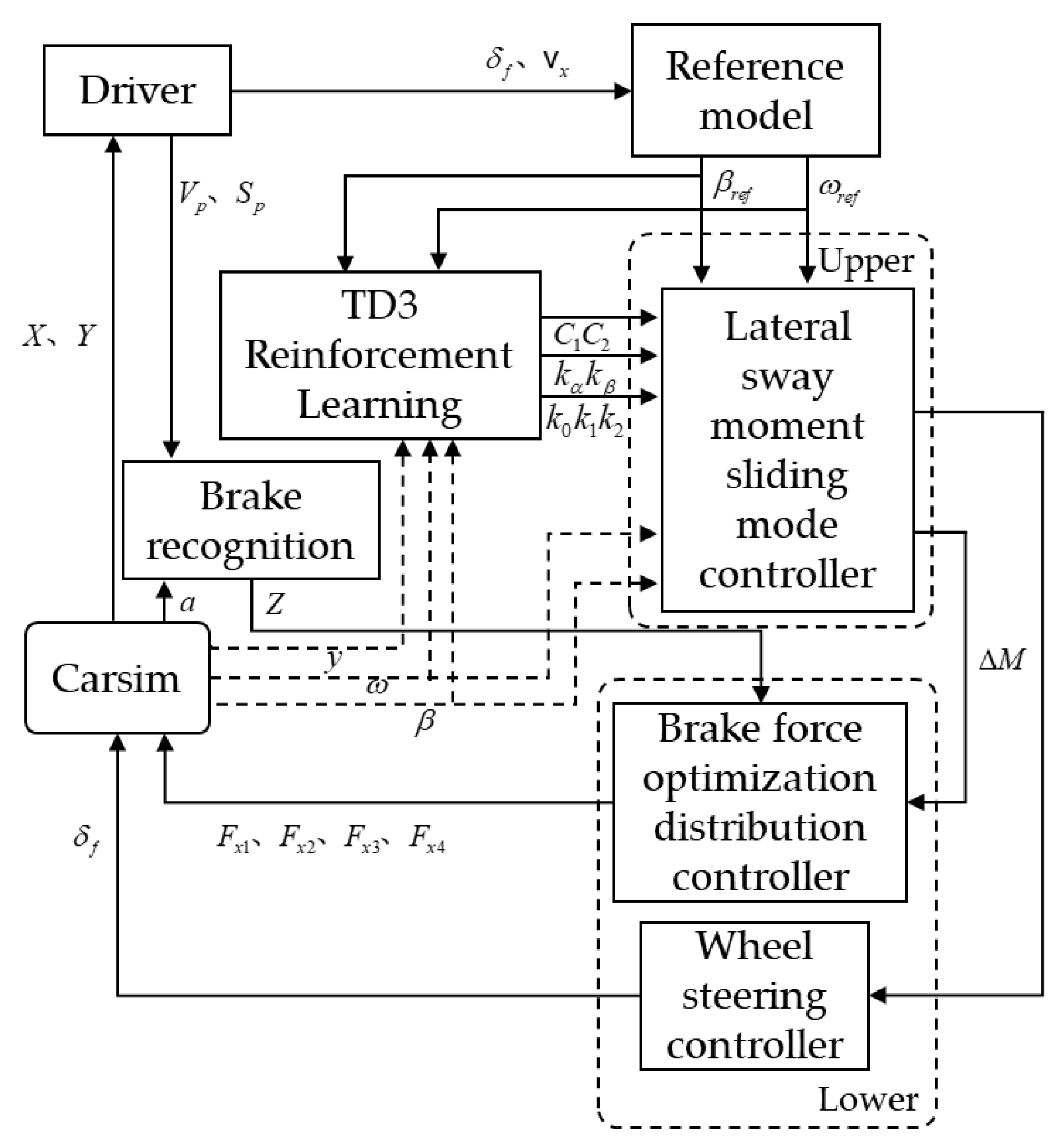
The overall control architecture of this paper is illustrated in Figure 10. The BP neural network identifies the braking intensity Z based on input vehicle speed, brake pedal displacement, and pedal velocity. The additional yaw moment, determined by the sliding mode controller optimized via the TD3 algorithm, is utilized to optimize braking force distribution. This strategy, integrated with active steering control, enables precise regulation of the vehicle’s yaw rate and lateral offset under failure conditions.

5. Results

Based on the analysis in Section 3 regarding the effects of braking intensity and brake system failure locations on vehicle stability, it can be concluded that a failure in the front brake system has a significant impact on vehicle stability during medium-to-high-intensity braking. Furthermore, the EMB system, which features independent control capabilities, exhibits a lower probability of multi-wheel brake failures. Therefore, this paper focuses on a simulation analysis of stability control in the event of a left front brake system failure under medium-to-high braking intensity conditions. The specific settings for the carsim simulation parameters are shown in Appendix A,

Table A3. Configuration of co-simulation parameters for Carsim and Simulink.

Parameters	Abbreviations and Units	Value
Vehicle quality	$m/(\mathrm{k}\mathrm{g})$	1895
Vehicle moment of inertia	$I_z/(\mathrm{k}\mathrm{g}\cdot {\mathrm{m}}^2)$	2031.4
Wheelbase	$c/(\mathrm{m})$	1.56
Distance from the front axle to the center of mass	$a/(\mathrm{m})$	1.15
Distance from the rear axle to the center of mass	$b/(\mathrm{m})$	1.52
Center of mass height	$h_g/(\mathrm{m})$	0.72
Front-wheel inertia	$I_f/(\mathrm{k}\mathrm{g}\cdot {\mathrm{m}}^2)$	1.9
Rear-wheel moment of inertia	$I_r/(\mathrm{k}\mathrm{g}\cdot {\mathrm{m}}^2)$	1.9
Unsprung mass of the front axle	$m_f/(\mathrm{k}\mathrm{g})$	150
Unsprung mass of the rear axle	$m_r/(\mathrm{k}\mathrm{g})$	118

.

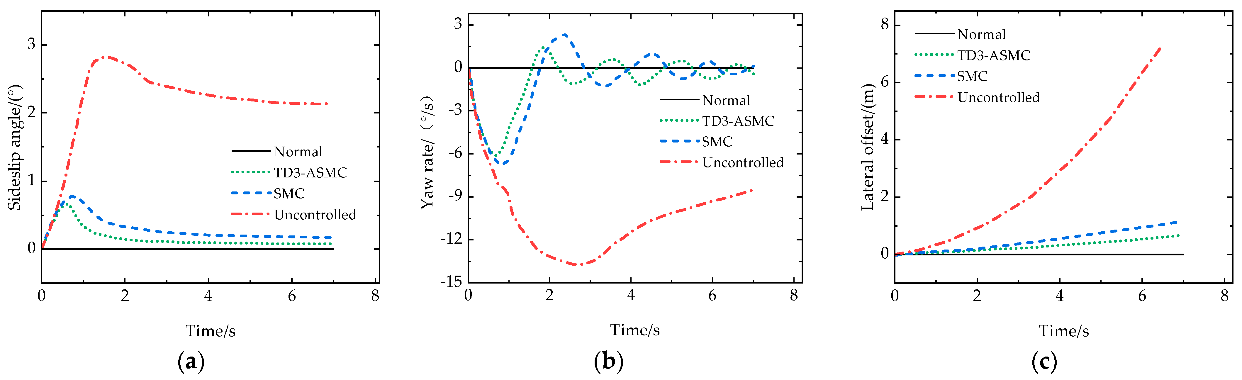
To validate the control effectiveness of secondary brake force distribution during a single-wheel brake failure and visually demonstrate the performance of the brake force distribution algorithm, this paper establishes four comparative scenarios: 1. Normal four-wheel braking (ideal condition). 2. Under a left front single-wheel brake failure, the upper layer employs TD3 adaptive sliding mode control (TD3-ASMC) to compute yaw moment. The lower-layer controller uses an optimization algorithm that takes into account braking force loss, yaw moment, and tire utilization to distribute braking force. 3. Under a single-wheel brake failure of the left front wheel, the upper layer employs standard SMC to calculate the yaw moment required for tracking sideslip angle and yaw rate, dynamically adjusting control weights. The lower layer uses an optimization algorithm that takes tire utilization into account to distribute braking force. 4. Vehicle with no control under a single-wheel brake failure of the left front wheel.

5.1. Comparison of Controller Outputs

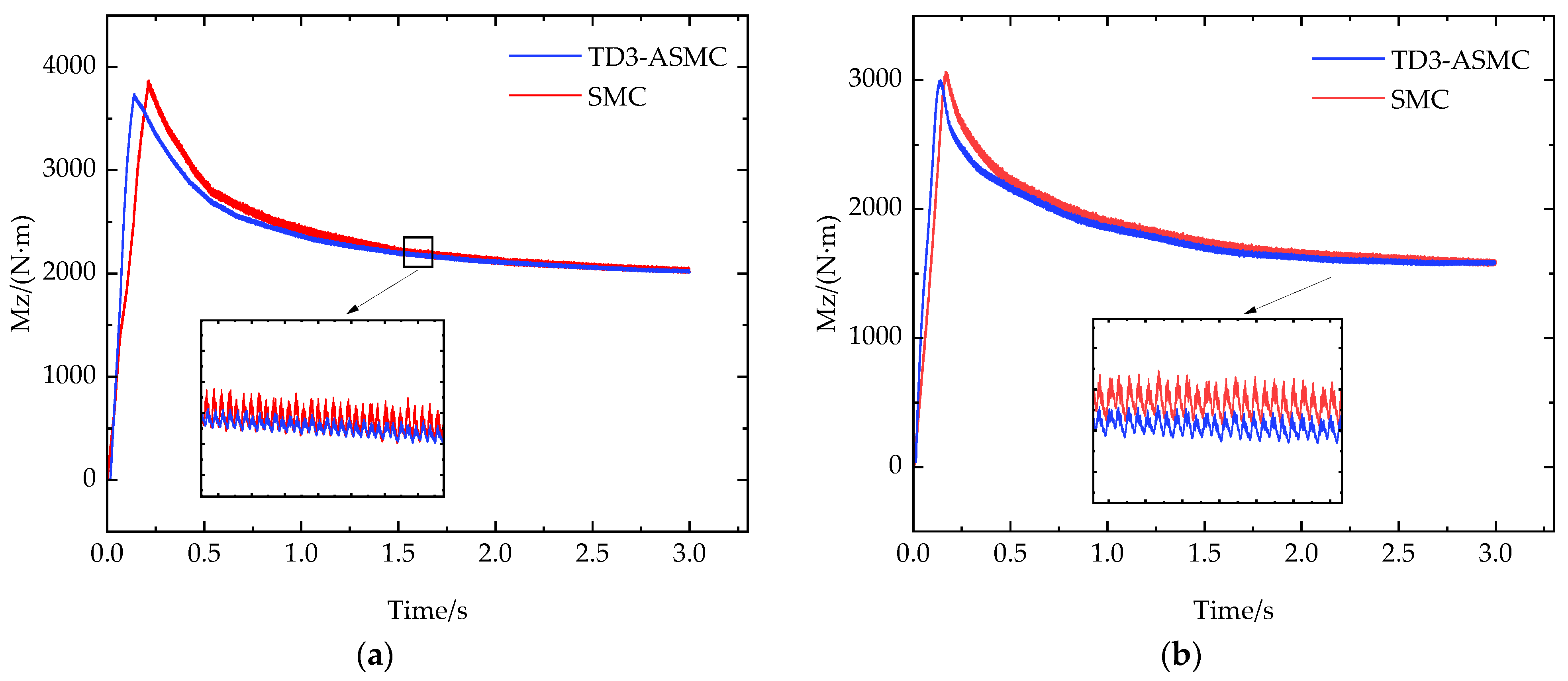
To visually demonstrate the effectiveness of the proposed TD3-ASMC strategy in suppressing sliding mode oscillations, Figure 11 shows the time response curves of the additional yaw moment ${\mathit{M}}_{\mathit{z}}$ (i.e., the control input signal) directly generated by the upper-layer controllers of the standard SMC and TD3-ASMC under straight-line and cornering conditions. Overall, both controllers respond quickly to yaw moment demands, but they exhibit significant differences in the high-frequency dynamic characteristics of the signals.

Examining the magnified section in Figure 11 reveals that the control output of the traditional SMC exhibits severe high-frequency, high-amplitude sawtooth-like chattering because it uses a discontinuous sign function sgn(s). In contrast, the control signal generated by TD3-ASMC exhibits significantly reduced high-frequency oscillation amplitude and is smoother. This indicates that the dynamic weighting smoothing reaching law introduced in the theoretical section of this paper, along with the reinforcement learning-based adaptive gain adjustment mechanism, has been successfully implemented, effectively softening the abrupt switching process of the control variable.

5.2. Straight-Line Braking Conditions

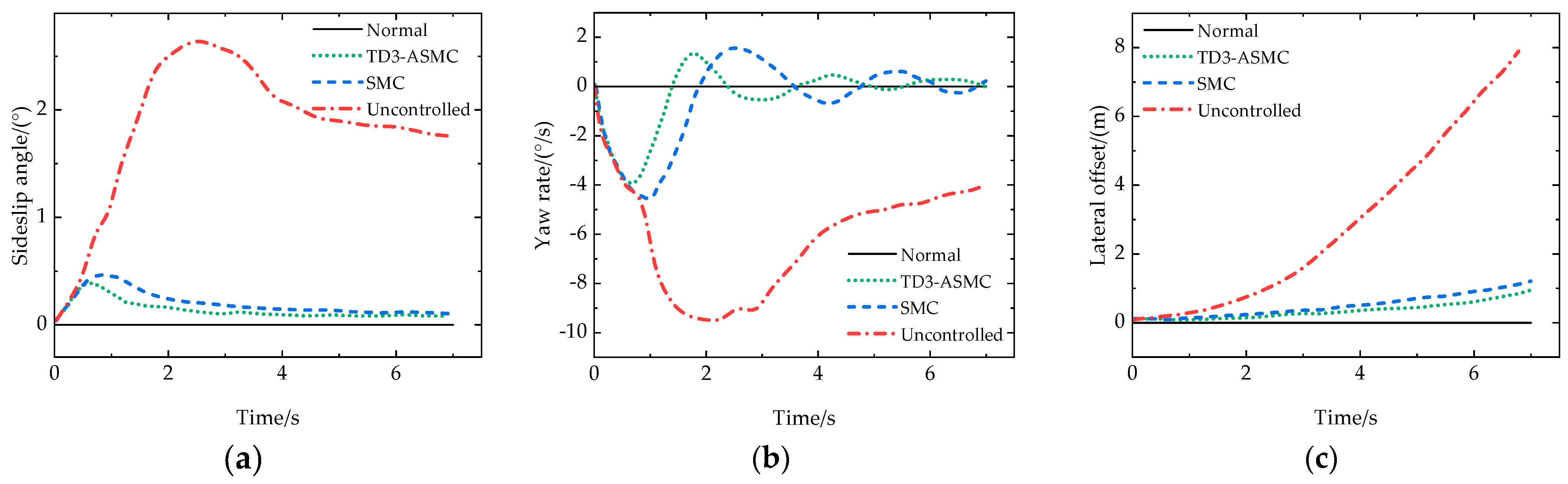
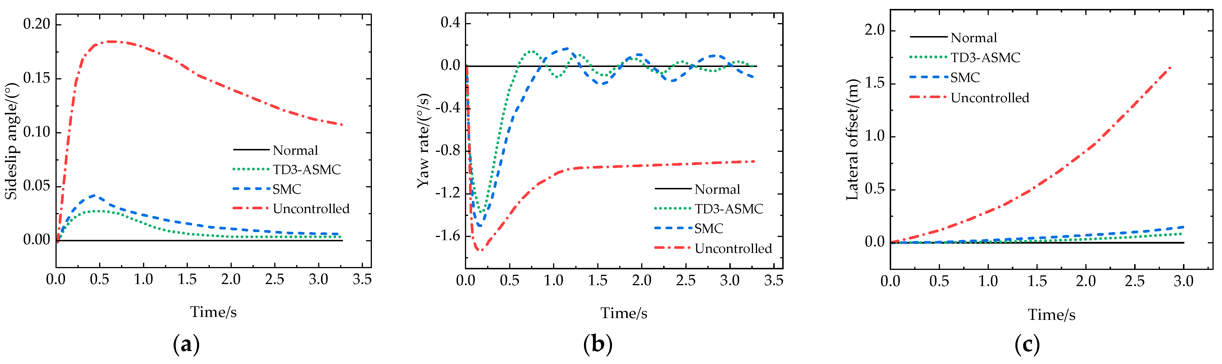
Figure 12 shows simulation results for a left front wheel brake failure on straight road surfaces with friction coefficients of $\mathit{\mu }=\mathbf{0.2}$ and 0.8. When the braking intensity is $\mathit{Z}=\mathbf{0.5}$, compared with the traditional SMC algorithm, the maximum sideslip angle of the vehicle controlled by the proposed algorithm decreased from 0.45$°$ to 0.39$°$. The maximum yaw rate decreased from 4.48$°/\mathbf{s}$ to 3.92$°/\mathbf{s}$, exhibiting a faster response. Meanwhile, the vehicle’s lateral offset decreased from 1.2 m to 0.96 m, remaining within the safety range ($<\mathbf{1.5} \mathbf{m}$).

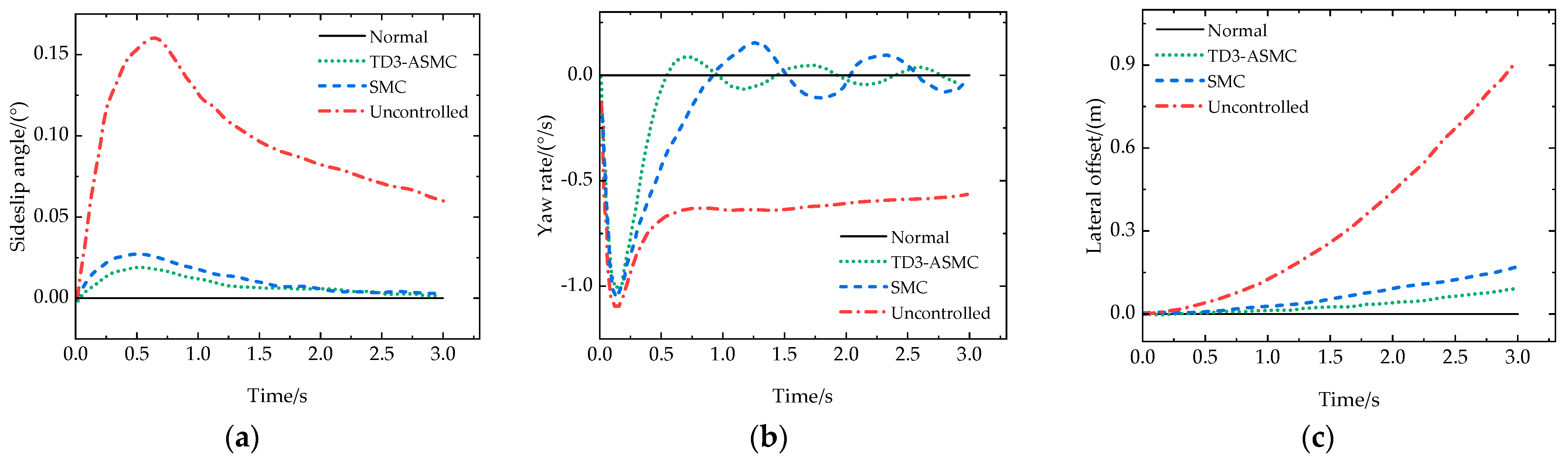
As shown in Figure 13, when the friction coefficient is $\mathit{\mu }=\mathbf{0.8}$, the maximum sideslip angle decreased from 0.027$°$ to 0.019$°$, and the maximum yaw rate decreased from 1.06$°/\mathbf{s}$ to 1.01$°/\mathbf{s}$, with a reduced fluctuation amplitude. The lateral offset also decreased from 0.169 m to 0.092 m.

Figure 14 and Figure 15 show the results of a braking maneuver with an intensity of $\mathit{Z}=\mathbf{0.8}$, performed at an initial speed of 60 km/h on a straight road surface with friction coefficients of 0.2 and 0.8, respectively, when the left front wheel fails. When the friction coefficient is 0.2, compared with the traditional algorithm, the maximum sideslip angle of the vehicle controlled by the proposed algorithm decreased from 0.77$°$ to 0.67$°$, the maximum yaw rate decreased from 6.7$°/\mathbf{s}$ to 6.1$°/\mathbf{s}$, and the lateral offset decreased from 1.16 m to 0.67 m. When the road friction coefficient is 0.8, the maximum sideslip angle decreased from 0.042° to 0.027°, the maximum yaw rate decreased from 1.49$°/\mathbf{s}$ to 1.37$°/\mathbf{s}$, and the lateral offset decreased from 0.15 m to 0.08 m.

In summary, when the left front wheel brake fails while driving on a straight road surface, the control strategy proposed in this paper outperforms traditional control algorithms in terms of sideslip angle, yaw rate, and lateral offset. It effectively prevents loss of control caused by unbalanced braking forces during brake failure and successfully suppresses vehicle lateral offset under such events.

5.3. Corner Braking Conditions

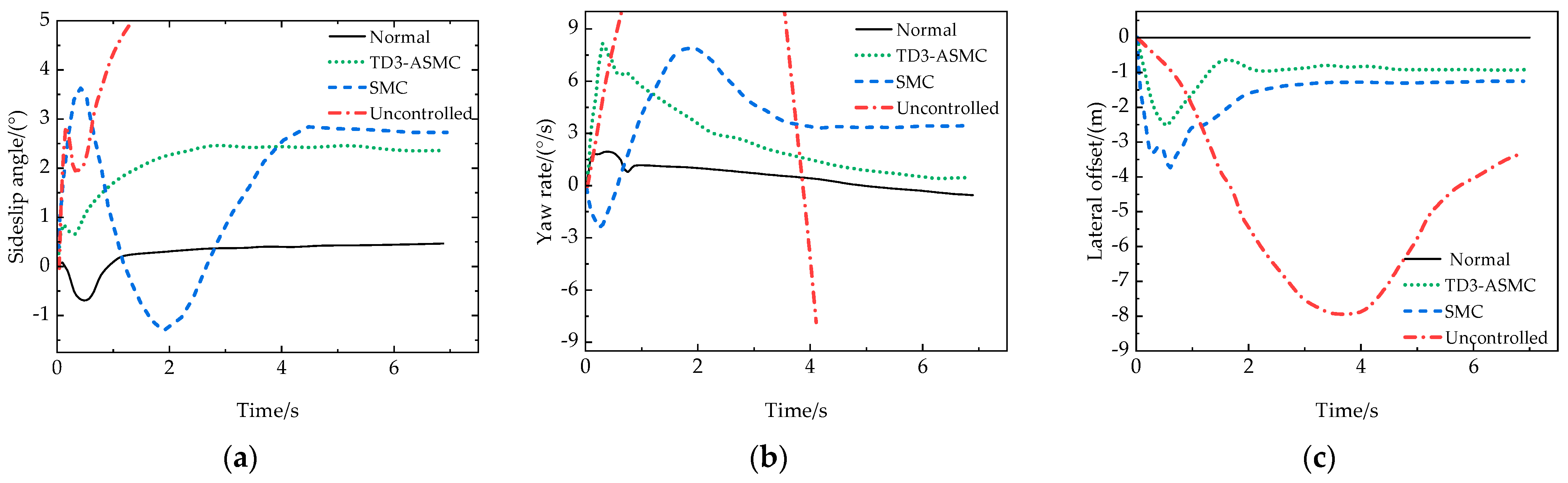
Figure 16 shows simulation results for left front wheel brake failure on curved road surfaces with friction coefficients of $\mathit{\mu }=\mathbf{0.2}$ and 0.8. When $\mathit{Z}=\mathbf{0.5}$, compared to the traditional SMC algorithm, the maximum sideslip angle of the vehicle controlled by the proposed algorithm decreased from 3.626$°$ to 2.457$°$, with significantly improved control response speed. Although the maximum yaw rate increased from 7.872$°/\mathbf{s}$ to 8.154$°/\mathbf{s}$, the overall yaw rate converged more quickly and exhibited a marked decrease in steady-state fluctuation. Meanwhile, the lateral offset of the vehicle decreased from 3.33 m to 2.5 m.

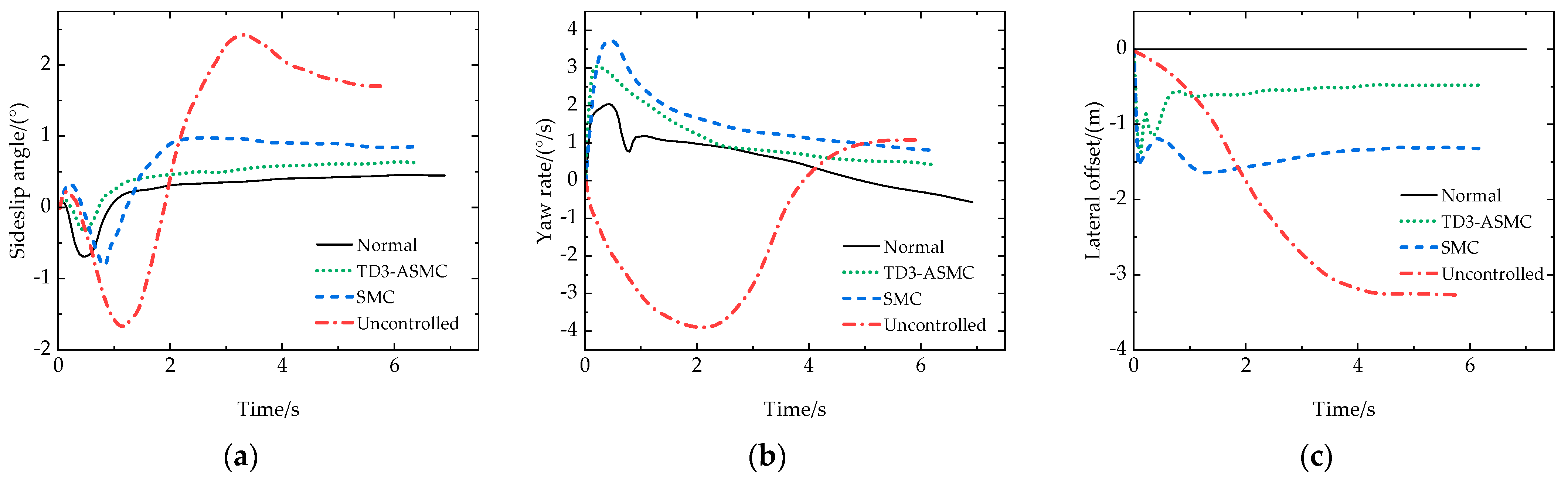
As shown in Figure 17, at a road friction coefficient of $\mathit{\mu }=\mathbf{0.8}$, the proposed control algorithm reduced the vehicle’s maximum sideslip angle from 0.976° to 0.474°, the maximum yaw rate from 3.72$°/\mathbf{s}$ to 3.04$°/\mathbf{s}$, and the lateral offset from 1.647 m to 1.373 m.

In summary, in the event of a left front brake system failure during cornering, the proposed control strategy outperforms traditional algorithms in terms of sideslip angle, yaw rate, and lateral offset. For the specific improvement details, please refer to

Table 2. Summary table comparing control effects of different algorithms.

Simulated Operating Conditions	Item	SMC	TD3-ASMC	Improvement
Straight road (μ = 0.2, Z = 0.5, V= 100 km/h)	Sideslip angle/(°)	0.45	0.39	13%
	Yaw rate/(°/s)	4.48	3.92	12.5%
	Lateral offset/m	1.20	0.93	20%
Straight road (μ = 0.8, Z = 0.5, V = 100 km/h)	Sideslip angle/(°)	0.027	0.019	29.6%
	Yaw rate/(°/s)	1.06	1.01	4.71%
	Lateral offset/m	0.169	0.092	45.6%
Straight road (μ = 0.2, Z = 0.8, V = 60 km/h)	Sideslip angle/(°)	0.77	0.66	14.3%
	Yaw rate/(°/s)	6.69	6.13	8.3%
	Lateral offset/m	1.16	0.67	42.2%
Straight road (μ = 0.8, Z = 0.8, V = 60 km/h)	Sideslip angle/(°)	0.042	0.027	35.7%
	Yaw rate/(°/s)	1.49	1.37	8.1%
	Lateral offset/m	0.151	0.086	43%
Curved road (μ = 0.2, Z = 0.5, V = 60 km/h)	Sideslip angle/(°)	3.626	2.457	32.2%
	Yaw rate/(°/s)	7.872	8.154	−3.6%
	Lateral offset/m	3.33	2.50	24.9%
Curved road (μ = 0.8, Z = 0.5, V = 60 km/h)	Sideslip angle/(°)	0.976	0.474	51.4%
	Yaw rate/(°/s)	3.72	3.04	18.3%
	Lateral offset/m	1.647	1.373	16.6%

. It effectively avoids the loss of control induced by unbalanced braking forces and successfully suppresses the vehicle’s lateral deviation under these critical conditions.

6. Conclusions

To address single-wheel brake failure on straight roads and curves, a hierarchical control strategy was designed considering factors such as road friction coefficient, braking intensity, and vehicle speed. The upper layer calculates the required yaw moment, while the lower layer optimizes braking force distribution among the functioning wheels. This effectively suppresses lateral offset and, in conjunction with active steering control, ensures that the vehicle can travel stably along the predetermined path. Simulation results indicate that the proposed control strategy significantly improves vehicle stability under extreme conditions, providing a new technical reference for enhancing active vehicle safety.

However, this study presents several limitations that should be acknowledged. First, the current simulation environment is relatively idealized and lacks consideration of real-world external disturbances. Second, although theoretical proofs and comparative simulation results have been provided for the proposed controller, a comprehensive robustness analysis has yet to be conducted. Furthermore, the scope of the selected driving scenarios is limited. The current evaluation solely addresses left front and left rear braking system failures during both straight-line driving and small-curvature cornering under varying speeds and adhesion coefficients. Consequently, vehicle stability under daily maneuvers (e.g., right-angle turns) and extreme conditions (e.g., fishhook test) requires further exploration. Moreover, complex road conditions, including non-uniform adhesion coefficients across all four wheels (e.g., split-friction surfaces) and sudden changes in road friction, should also be considered.

Future research will focus on real-vehicle testing to incorporate actual physical disturbances. We also plan to evaluate the algorithm’s control performance under simultaneous failures of dual- or multi-wheel braking systems at various positions, as well as under demanding driving conditions like right-angle turns and uneven road adhesion. Finally, a detailed robustness analysis will be performed to further demonstrate the reliability of the proposed control strategy.

References

1. Zhou, S.W.; Liu, J.S.; Wang, Z.L.; Sun, S.H. Research on Design Optimization and Simulation of Regenerative Braking Control Strategy for Pure Electric Vehicle Based on Emb Systems. Trans. FAMENA 2023, 47, 33–49. [Google Scholar] [CrossRef]
2. Xu, Z.; Gerada, C. Enhanced Estimation of Clamping-Force for Automotive EMB Actuators Using a Switching Extended State Observer. IEEE Trans. Ind. Electron. 2024, 71, 2220–2230. [Google Scholar] [CrossRef]
3. Li, C.C.; Zhuo, G.R.; Tang, C.; Xiong, L.; Tian, W.; Qiao, L.; Cheng, Y.L.; Duan, Y.L. A Review of Electro-Mechanical Brake (EMB) System: Structure, Control and Application. Sustainability 2023, 15, 38. [Google Scholar] [CrossRef]
4. Zheng, L.F.; Lu, Y.J.; Wang, J.X.; Li, H.Y. Braking failure anti-rollover control and hardware-in-the-loop verification of wire-controlled heavy vehicles. Sci. Rep. 2024, 14, 17. [Google Scholar] [CrossRef]
5. Kim, S.; Huh, K. Fault-tolerant braking control with integerated EMBs and regenerative in-wheel motors. Int. J. Automot. Technol. 2016, 17, 923–936. [Google Scholar] [CrossRef]
6. Argha, A.; Su, S.W.; Zheng, W.X.; Celler, B.G. Sliding-mode fault-tolerant control using the control allocation scheme. Int. J. Robust Nonlinear Control 2019, 29, 6256–6273. [Google Scholar] [CrossRef]
7. Zhou, J.; Di, Y.G.; Miao, X.L. Single-Wheel Failure Stability Control for Vehicle Equipped with Brake-by-Wire System. World Electr. Vehicle J. 2023, 14, 16. [Google Scholar] [CrossRef]
8. Zhang, L.P.; Pang, Z.W.; Wang, S.; Zhang, S.L.; Yuan, X.M. Electromechanical composite brake control for two in-wheel motors drive electric vehicle with single motor failure. Proc. Inst. Mech. Eng. Part D-J. Automob. Eng. 2020, 234, 1057–1074. [Google Scholar] [CrossRef]
9. Pang, H.; Liu, M.H.; Hu, C.; Liu, N. Practical Nonlinear Model Predictive Controller Design for Trajectory Tracking of Unmanned Vehicles. Electronics 2022, 11, 18. [Google Scholar] [CrossRef]
10. Zhou, X.Y.; Wang, Z.J.; Wang, J.M. Automated Vehicle Path Following: A Non-Quadratic-Lyapunov-Function-Based Model Reference Adaptive Control Approach with e∞-Smooth Projection Modification. IEEE Trans. Intell. Transp. Syst. 2022, 23, 21653–21664. [Google Scholar] [CrossRef]
11. Ito, A.; Azuma, S.I. Autonomous distributed braking and driving force control architecture based on broadcast control for vehicles with in-wheel motors on four wheels. Adv. Robot. 2024, 38, 672–683. [Google Scholar] [CrossRef]
12. Xiao, L.; Hu, Y.M.; Zeng, D.Q.; Yu, Y.Q.; Han, K.L.; Yang, J.W.; Liu, W.D. A study on lateral stability control of distributed drive electric vehicle based on fast adaptive super-twisting sliding mode control. Proc. Inst. Mech. Eng. Part D-J. Automob. Eng. 2026, 240, 2624–2639. [Google Scholar] [CrossRef]
13. Geng, G.Q.; Cheng, P.; Sun, L.Q.; Xu, X.; Shen, F.Q. A Study on Lateral Stability Control of Distributed Drive Electric Vehicle Based on Fuzzy Adaptive Sliding Mode Control. Int. J. Automot. Technol. 2024, 25, 1415–1429. [Google Scholar] [CrossRef]
14. Wu, T.; Wang, J.N.; Rong, J.; Meng, Y.; Yang, X.J.; Peng, J.; Chu, L. Braking reconstruction control for fault-tolerance in electro-mechanical brake actuator failures. Proc. Inst. Mech. Eng. Part D-J. Automob. Eng. 2025, 239, 6455–6470. [Google Scholar] [CrossRef]
15. Ha, Y.; Jeon, S.; Park, J.; Choi, S.; Woo, S. Coordinated Control Approach for Brake Actuator Failures: A Fault-Tolerant Strategy Using Braking Systems and Steering. IEEE Access 2025, 13, 108005–108024. [Google Scholar] [CrossRef]
16. Yang, K.; Dong, D.X.; Ma, C.; Tian, Z.X.; Chang, Y.L.; Wang, G. Stability Control for Electric Vehicles with Four In-Wheel-Motors Based on Sideslip Angle. World Electr. Vehicle J. 2021, 12, 15. [Google Scholar] [CrossRef]
17. Peng, Z.X.; Ning, G.T. 2 DOF Lateral Dynamic Model with Force Input of Skid Steering Wheeled Vehicle. In Proceedings of the IEEE Transportation Electrification Conference and Expo (ITEC Asia-Pacific), Beijing, China, 31 August–3 September 2014; IEEE: Piscataway, NJ, USA, 2014. [Google Scholar]
18. Barbaro, M.; Genovese, A.; Timpone, F.; Sakhnevych, A. Extension of the multiphysical magic formula tire model for ride comfort applications. Nonlinear Dyn. 2024, 112, 4663–4685. [Google Scholar] [CrossRef]
19. Paschoal, W.; Souza, I.; Torres, L.; Murilo, A.; Ozelo, R. Comparative Study of Tire Models Applied to Electronic Stability Control in Automotive Simulator. IEEE Latin Am. Trans. 2024, 22, 835–841. [Google Scholar] [CrossRef]
20. Tang, J.H.; Zuo, Y.Y. Braking Intention Recognition Method Based on the Fuzzy Neural Network. Wirel. Commun. Mob. Comput. 2022, 2022, 8. [Google Scholar] [CrossRef]
21. Tang, M.B.; Zhang, X.W. Optimal Regenerative Braking Control Strategy for Electric Vehicles Based on Braking Intention Recognition and Load Estimation. IEEE Trans. Veh. Technol. 2024, 73, 3378–3392. [Google Scholar] [CrossRef]
22. Chen, Z.R.; Ding, R.K.; Zhou, Q.; Wang, R.C.; Zhao, B.G.; Liao, Y.S. Research on coordinated control of electro-hydraulic composite braking for an electric vehicle based on the Fuzzy-TD3 deep reinforcement learning algorithm. Control Eng. Pract. 2025, 157, 26. [Google Scholar] [CrossRef]
23. Wu, D.M.; Zhang, Q.; Du, C.Q.; Li, Y. Path tracking and stability control of 4WID electric vehicles based on variable prediction horizon MPC. Int. J. Veh. Des. 2024, 95, 30. [Google Scholar] [CrossRef]
24. Krishnan, S.G.; Kumar, P.S.; Matara, N.N.; Wang, Y. Real-Time Experimental Evaluation and Analysis of PID and MPC Controllers Using HIL Setup for Robust Steering System of Autonomous Vehicles. IEEE Access 2024, 12, 74711–74723. [Google Scholar] [CrossRef]
25. Ding, S.H.; Wang, J.D.; Zheng, W.X. Second-Order Sliding Mode Control for Nonlinear Uncertain Systems Bounded by Positive Functions. IEEE Trans. Ind. Electron. 2015, 62, 5899–5909. [Google Scholar] [CrossRef]
26. Chen, J.; Han, Y.; Huangfu, B.; Shi, J. Research on Vehicle Stability Control Strategy Under Single-Wheel Emb Braking Failure. In Proceedings of the 2024 8th CAA International Conference on Vehicular Control and Intelligence (CVCI), Chongqing, China, 25–27 October 2024; IEEE: Piscataway, NJ, USA, 2024; pp. 1–6. [Google Scholar]
27. Zhang, X.Q.; Li, J.; Ma, Z.G.; Chen, D.M.; Zhou, X.X. Lateral Trajectory Tracking of Self-Driving Vehicles Based on Sliding Mode and Fractional-Order Proportional-Integral-Derivative Control. Actuators 2024, 13, 21. [Google Scholar] [CrossRef]
28. Qin, Z.B.; Jing, H.D.; Chen, L.; Hu, M.J.; Bian, Y.G.; Cui, Q.J. Longitudinal Vehicle Stability Control Based on Modified Sliding Mode Control. Automot. Innov. 2024, 7, 335–348. [Google Scholar] [CrossRef]
29. Shtessel, Y.; Plestan, F.; Edwards, C. Adaptive Sliding Mode and Second Order Sliding Mode Control with Applications: A Survey. In Proceedings of the 22nd World Congress of the International Federation of Automatic Control (IFAC), Yokohama, Japan, 9–14 July 2023; pp. 761–772. [Google Scholar]
30. Sun, C.G.; Sun, Z.Y.; Liu, J.Q. Electro-hydraulic servo sliding mode control integrating TD3 intelligent optimization and adaptive fractional order. Mach. Tool Hydraul. 2025, 53, 108–117. [Google Scholar] [CrossRef]
31. Zhang, H.J.; Wang, Z.L. PID parameter optimization based on TD3 algorithm of double replay buffer. Control Theory Appl. 2026, 43, 139–148. [Google Scholar] [CrossRef]
32. Zhong, H.J.; Wang, Z.L. TD3 Algorithm of Dynamic Classification Replay Buffer Based PID Parameter Optimization. Int. J. Control Autom. Syst. 2024, 22, 3068–3082. [Google Scholar] [CrossRef]
33. Chen, Y.X.; Gai, J.T.; He, S.; Li, H.H.; Cheng, C.; Zou, W.J. MPC-TD3 Trajectory Tracking Control for Electrically Driven Unmanned Tracked Vehicles. Electronics 2024, 13, 16. [Google Scholar] [CrossRef]
34. Wang, H.L.; Tao, H.D.; Pi, D.W.; Wang, W.H.; Chen, Y.J.; Wang, X.H. Coordinated longitudinal and vertical control of corner module vehicles based on ground-tyre adhesion on rugged slopes. Int. J. Veh. Des. 2025, 97, 27. [Google Scholar] [CrossRef]
35. Ma, X.B.; Wong, P.K.; Zhao, J.; Xie, Z.C. Multi-Objective Sliding Mode Control on Vehicle Cornering Stability with Variable Gear Ratio Actuator-Based Active Front Steering Systems. Sensors 2017, 17, 16. [Google Scholar] [CrossRef] [PubMed]
Figure 1. Seven-DOF vehicle dynamics model.
Wevj 17 00230 g001
Figure 2. Two-DOF vehicle reference model.
Wevj 17 00230 g002
Figure 3. Vehicle stability simulation. (a) Vehicle stability with left front brake failure. (b) Vehicle stability with rear right brake failure.
Wevj 17 00230 g003
Figure 4. BP neural network structure.
Wevj 17 00230 g004
Figure 5. The relationship between the training effect of the BP neural network and the number of neurons in the hidden layers.
Wevj 17 00230 g005
Figure 6. Model identification accuracy.
Wevj 17 00230 g006
Figure 7. Variation curves of system under two different convergence laws.
Wevj 17 00230 g007
Figure 8. TD3 reinforcement learning framework.
Wevj 17 00230 g008
Figure 9. TD3 training curve.
Wevj 17 00230 g009
Figure 10. Control process.
Wevj 17 00230 g010
Figure 11. Comparison of controller outputs. (a) Z = 0.5 ,   μ = 0.8 ,   V = 100   k m / h  Straight. (b) Z = 0.5 ,   μ = 0.8 ,   V = 100   k m / h  curve.
Wevj 17 00230 g011
Figure 12. Simulation results for a vehicle with a braking intensity of Z = 0.5 , an initial speed of 100 km/h, and a road surface with a coefficient of friction of 0.2. (a) Sideslip angle. (b) Yaw rate. (c) Lateral offset.
Wevj 17 00230 g012
Figure 13. Simulation results for a vehicle with a braking intensity of Z = 0.5 , an initial speed of 100 km/h, and a road surface with a coefficient of friction of 0.8. (a) Sideslip angle. (b) Yaw rate. (c) Lateral offset.
Wevj 17 00230 g013
Figure 14. Simulation results for a vehicle with a braking intensity of Z = 0.8 , an initial speed of 60 km/h, and a road surface with a coefficient of friction of 0.2. (a) Sideslip angle. (b) Yaw rate. (c) Lateral offset.
Wevj 17 00230 g014
Figure 15. Simulation results for a vehicle with a braking intensity of Z = 0.8 , an initial speed of 60 km/h, and a road surface with a coefficient of friction of 0.8. (a) Sideslip angle. (b) Yaw rate. (c) Lateral offset.
Wevj 17 00230 g015
Figure 16. Simulation results for a vehicle with a braking intensity of Z = 0.5 , an initial speed of 60 km/h, and a road surface with a coefficient of friction of 0.2. (a) Sideslip angle. (b) Yaw rate. (c) Lateral offset.
Wevj 17 00230 g016
Figure 17. Simulation results for a vehicle with a braking intensity of Z = 0.5 , an initial speed of 60 km/h, and a road surface with a coefficient of friction of 0.8. (a) Sideslip angle. (b) Yaw rate. (c) Lateral offset.
Wevj 17 00230 g017