Heuristic Algorithms for Heterogeneous and Multi-Trip Electric Vehicle Routing Problem with Pickup and Delivery

Abstract

In light of the widespread use of electric vehicles for urban distribution, this paper delves into the electric vehicle routing problem (EVRP): specifically addressing multiple trips per vehicle, diverse vehicle types, and simultaneous pickup and delivery. The primary objective is to minimize the overall cost, which encompasses travel expenses, waiting times, recharging costs, and fixed vehicle costs. The focal problem is formulated as a heterogeneous and multi-trip electric vehicle routing problem with pickup and delivery (H-MT-EVRP-PD). Additionally, we introduce two heuristic algorithms to efficiently approximate solutions within a reasonable computational time. The variable neighborhood search (VNS) algorithm and the adaptive large neighborhood search (ALNS) algorithm are presented and compared based on our computational experiences with both. Through solving a series of large-scale real-world instances for the H-MT-EVRP-PD and smaller instances using an exact method, we demonstrate the efficacy of the proposed approaches.

1. Introduction

1.1. Motivation

The vehicle routing problem (VRP) stands as a pivotal research focus within the logistics domain. Given the rapid expansion of logistics and express enterprises in recent years, addressing the challenge of optimizing routing amidst multiple constraints and a substantial task volume has emerged as a prominent research area. Concurrently, heightened societal emphasis on environmental preservation has led logistics and express enterprises to adopt electric vehicles for distribution, particularly in urban settings due to the operational constraints associated with limited range.

This paper is motivated by the context of express package distribution in urban areas, where external packages continually arrive at a city distribution center (depot) serving as the launchpad for last-mile delivery operations. Consequently, daily optimization of distribution from the depot to customers becomes imperative and necessitates consideration of various attributes in the optimization process. Key considerations include: (1) The delivery window spans from 6:00 to 24:00, prompting the need for multiple trips per vehicle per day to accommodate limited capacity and to minimize the fleet size, thereby reducing fixed vehicle costs. (2) Logistics distribution, such as express packages, involves both pickup and delivery requirements, introducing the crucial aspect of the pickup and delivery problem (PDP). (3) Enterprises often deploy a variety of electric vehicle types. While larger vehicles may fulfill transportation demands without recharging operations, the cost-effectiveness of incorporating smaller vehicles in the fleet mix can reduce overall costs. Consequently, fleet managers must consider heterogeneous vehicle types.

Addressing these concerns, this paper introduces a novel multi-attribute vehicle routing problem: the heterogeneous and multi-trip electric vehicle routing problem with pickup and delivery (H-MT-EVRP-PD). It amalgamates well-established problems, including the heterogeneous vehicle routing problem (HVRP), multi-trip vehicle routing problem (MTVRP), pickup and delivery problem (PDP) for goods transportation, and the recently defined electric vehicle routing problem with time windows and recharging stations (E-VRPTW).

1.2. Contributions of This Paper

This paper makes significant contributions to the field, encompassing a formal problem description, a mixed-integer programming model, and two heuristic frameworks. Comprehensive computational experiments are conducted for the heterogeneous and multi-trip electric vehicle routing problem with pickup and delivery (H-MT-EVRP-PD). The main contributions are summarized as follows:

(1)

Problem Formulation: This paper unifies research on the heterogeneous vehicle routing problem (HVRP), multi-trip vehicle routing problem (MTVRP), pickup and delivery problem (PDP), and electric vehicle routing problem with time windows and recharging stations (E-VRPTW). It introduces a novel problem: the heterogeneous and multi-trip electric vehicle routing problem with pickup and delivery (H-MT-EVRP-PD).

(2)

Mixed-Integer Programming Model: To precisely describe the problem, we formulate the H-MT-EVRP-PD as a mixed-integer programming model. This model is directly applicable to small instances and can be solved efficiently by commercial solvers.

(3)

Heuristic Approaches: Recognizing the challenge of larger real-world instances, we introduce two heuristic frameworks: the variable neighborhood search (VNS) algorithm and the adaptive large neighborhood search (ALNS) algorithm.

(4)

Computational Experiments: Our approach demonstrates its effectiveness by yielding optimal solutions for small instances and providing high-quality feasible solutions for larger instances. A sensitivity analysis that examines the impact of service time, vehicle volume, and driving range is conducted through additional experiments.

The structure of the paper is organized as follows:

Section 2 presents a concise review of related works in the field. Section 3 provides a mixed-integer programming formulation with detailed formal notations. Section 4 outlines the solution procedures for the proposed VNS and ALNS approaches. Section 5 presents comprehensive computational results from experiments. Section 6 concludes the paper and discusses potential future directions.

2. Literature Review

Some scholars recently studied the routing problems related to this paper, such as multi-trip time-dependent vehicle routing problem with time windows [1], the pickup and delivery problem with time windows [2], the electric fleet size and mix vehicle routing problem with time windows [3], and the electric vehicle routing problem with time windows and recharging stations [4]. In practice, for the distribution of electric vehicles in an urban area, logistics and express enterprises need to consider not only the limited driving range and long recharging time of electric vehicles but also multiple trips, heterogeneous vehicles, and pickup and delivery to reduce costs and improve distribution efficiency. To the best of our knowledge, there is no scholarly integration of the attributes of electric, multi-trip, heterogeneous, and pickup and delivery to conduct the vehicle routing problem so far. This paper tries to combine the problems of HVRP, MTVRP, PDP, and EVRPTW, and the subsequent review will focus on these four problems.

2.1. Related Works on the Electric Vehicle Routing Problem with Time Windows

The electric vehicle routing problem with time windows (EVRPTW) is a variant of the classical vehicle routing problem with time windows (VRPTW) for which the load tools are electric vehicles (EVs); it was first introduced by [4]. Moreover, Schneider (2014) [4] designed a heuristic algorithm based on the variable neighborhood search (VNS) and tabu search (TS) to address the proposed variant. On this basis, Ref. [3] proposed vehicle routing problems with various types of electric vehicles by considering service time window and recharging station selection. Ref. [5] put forward the problem of location selection and route selection of electric vehicle power stations by considering the limitation of battery driving range and designed a four-stage heuristic algorithm. According to [6], a corresponding integer programming model was established to optimize the location and distribution routing of electric vehicle logistics distribution systems. Ref. [7] constructed an optimization model for electric vehicle distribution routing with time windows with the goal of minimizing the total cost. Ref. [8] constructed an urban distribution routing optimization model based on pure electric vehicles in a social charging network with vehicle capacity constraints, single charge driving mileage constraints, and so on.

The use of different recharging technologies has been considered in the literature. For instance, to reduce recharging duration, Ref. [9] allowed partial recharging instead of full recharging to make the distribution route more flexible and developed an adaptive large neighborhood search algorithm to solve the proposed model effectively. Ref. [10] proposed a non-deterministic simulated annealing framework to solve the electric vehicle routing problem in which multiple technologies used for recharging are considered. Ref. [11] argued that the recharging level of the battery was a non-linear function of the recharging time and then raised a hybrid metaheuristic for the problem. Ref. [12] introduces the electric vehicle routing problem with shared charging stations, which is solved by a multistart heuristic that performs an adaptive large neighborhood search.

2.2. Related Works on the Vehicle Routing Problem with a Heterogeneous Fleet

This section considers the variant of the VRP in which a heterogeneous fleet of vehicles, each possibly having a different capacity and cost, is available for the distribution activities. Several specific variants have been developed over time to consider the two main features of this problem. On the one hand, there is the strategic issue of finding the best combination of vehicles to be used for the long-term sizing of a fleet. This results in fleet size and mix (FSM) problems, in which the vehicle fleet is assumed to be unlimited. On the other hand, one can consider the tactical issue of using the most appropriate vehicles from a limited fleet, which results in the heterogeneous VRP (HVRP). This paper focuses on the latter. In the literature, the terms heterogeneous or mixed fleet VRP (HFVRP) are also used to identify the whole problem family [13]. Ref. [14] discussed the heterogeneous vehicle routing problem and proposed several effective heuristic solutions and techniques to generate the lower bound of the optimal solution to solve the problem. Ref. [15] provided an overview of an approach to solve the heterogeneous vehicle routing problem and classified the variants of the problem described in the literature.

Time windows are also considered in the problem. Ref. [16] proposed a new three-phase heuristic method to solve the heterogeneous and multi-depot vehicle routing problem with time windows. Ref. [17] proposed a new two-phase solution framework based on a mixed tabu search to solve the heterogeneous fleet routing problem with time windows. Ref. [18] considered a real-life heterogeneous fleet vehicle routing problem with time windows and split deliveries that occurred for a major Brazilian retail group and significantly reduced distribution costs by using a scatter search approach. Ref. [19] investigated the heterogeneous vehicle routing problem with limited number of vehicles and time windows and proposed a method based on a tabu search algorithm. Recently, Ref. [3] introduced an electric fleet size and mixed vehicle routing problem with time windows and recharging stations in which the number of vehicles of each type was unlimited.

2.3. Related Works on the Multi-Trip Vehicle Routing Problem

Vehicle routing problems with multiple trips feature more than one trip per vehicle during operation. Many studies have investigated MTVRP variants with different heuristic algorithms, such as a multi-phase constructive heuristic enhanced by a suitable data structure [20], adaptive memory algorithm [21], hybrid genetic algorithm [22], adaptive large neighborhood search [23], and combination of vehicle routing heuristics with bin packing routing [24]. In addition, the time window has also been considered. Ref. [25] described an exact algorithm for a single-vehicle routing problem with time windows and multiple routes. Ref. [26] addressed the multi-trip vehicle routing problem with time windows and released dates through a population-based algorithm with a giant tour representation for individuals. Ref. [27] found a new exact algorithm to solve the multi-trip vehicle routing problem with time windows and limited duration.

2.4. Related Works on the Vehicle Routing Problem with Pickup and Delivery

In this new problem, backhauls are not restricted to be visited once all linehaul customers have been served; neither are backhaul customers fully mixed with linehaul customers.

Another variant of the VRP is the pickup and delivery problem [28], in which vehicles transport goods from a pickup location to a corresponding delivery location. In the vehicle routing problem with pickup and delivery, a set of vehicles must be optimally routed to service a set of transportation demands subject to constraints on capacities, time windows, precedence, and so on. Ref. [29] developed a multi-objective vehicle routing and scheduling heuristic for a pickup and delivery problem that assigned customers to more than one vehicle and allocated more than one customer to a vehicle at a time. Ref. [30] proposed a reactive tabu search approach to work out the pickup and delivery problem with time windows. Ref. [31] applied column generation to figure out the linear relaxation of a set-partitioning type formulation from the pickup and delivery vehicle routing problem. Ref. [32] proposed a heuristic based on an extension of the large neighborhood search heuristic mentioned earlier that consisted of numerous competing subheuristics for the problem. Ref. [33] presented a new exact algorithm for solving the pickup and delivery problem with time windows based on a set-partitioning integer formulation. Sartori and Buriol (2020) [2] proposed a metaheuristic for the pickup and delivery problem with time windows that presents the use of well-known heuristic components embedded in an iterated local search framework.

3. Problem Description and Formulation

The heterogeneous and multi-trip electric vehicle routing problem with pickup and delivery (H-MT-EVRP-PD) can be formulated as follows. Let N be a set of customers, F be a set of recharging stations, and $N^{\prime }$ be a set of nodes, with $N^{\prime }=N\cup F^{\prime }$, where $F^{\prime }$ denotes a set of dummy nodes generated to permit multiple visits to each node in the set F of recharging stations. Nodes 0 and $n+1$ denote the same depot, and each route starts at 0 and ends at $n+1$. To indicate that a set contains the respective instance of the depot, the set is subscripted with 0 and $n+1$; i.e., $F_0^{\prime }=F^{\prime }\cup \{0\}$ denotes the set of recharging visits and depot 0, $N_0^{\prime }=N^{\prime }\cup \{0\}$ is the set of customers and recharging visits and depot 0, $N_{n+1}^{\prime }=N^{\prime }\cup \{n+1\}$ is the set of customers and recharging visits and depot $n+1$, and $N_{0,n+1}^{\prime }=N^{\prime }\cup \{0\}\cup \{n+1\}$ is the set of customers and recharging visits including depot nodes 0 and $n+1$. Therefore, the problem of interest H-MT-EVRP-PD can be defined on a weighted directed graph $G=(N_{0,n+1}^{\prime },A)$ with the set of arcs $A=\{(i,j)|i,j\in N_{0,n+1}^{\prime },i\ne j\}$. Each arc is associated with a distance $D_{ij}$ and a travel time $T_{ij}^k$ of type k. Parameters $M{C}^k$ and $M{V}^k$ represent the maximum load and maximum volume, respectively, of vehicle type k. Each node $i\in N_0$ is associated with a demand capacity $Q_i$, a demand volume $V_i$, and a service time window $[E_i,L_i]$. The time interval $[E_0,L_0]$ represents a workday. Let $H^{kg}$ be the set of possible trips for the vehicle g of type k during the workday, and then the combination $(kg,u)$ represents the u-th trip performed by the vehicle g of type k.

3.1. Parameter Settings

This paper uses driving range to measure the battery capacity. Decision variables, subscripts, and parameters used in the mathematical formulation are listed as follows.

Decision Variables

• $x_{iju}^{kg}$: binary decision variable indicating whether vehicle g of type k travels arc $(i,j)$ in trip u;
• $t_{iu}^{kg}$: decision variable of arrival time of vehicle g of type k at node i in trip u;
• $m_{iu}^{kg}$: decision variable of current load of vehicle g of type k at node i in trip u;
• $c_{iu}^{kg}$: decision variable of current volume of vehicle g of type k at node i in trip u;
• $y_{iu}^{kg}$: decision variable of remaining range of vehicle g of type k at node i in trip u.

Subscripts and Parameters

• N: set of customers $N=1,2,\cdots ,n$;
• F: set of recharging stations;
• $0,n+1$: index of start and end depot nodes;
• $\overline{N}$: set of customers without waiting times;
• $N_0$: set of customers and start depot 0;
• $F^{\prime }$: set of dummy nodes, i.e., multiple visits for recharging stations F;
• $N^{\prime }$: set of customers and recharging visits, $N^{\prime }=N\cup F^{\prime }$;
• $F_0^{\prime }$: set of recharging visits and depot 0, $F_0^{\prime }=F^{\prime }\cup 0$;
• $N_0^{\prime }$: set of customers and recharging visits and depot 0, $N_0^{\prime }=N^{\prime }\cup 0$;
• $N_{n+1}^{\prime }$: set of customers and recharging visits and depot $n+1$, $N_{n+1}^{\prime }=N^{\prime }\cup n+1$;
• $N_{0,n+1}^{\prime }$: set of customers and recharging visits and depot nodes 0 and $n+1$, $N_{0,n+1}^{\prime }=N^{\prime }\cup 0\cup n+1$;
• K: set of vehicle types;
• $I^k$: set of vehicles of type k, $k\in K$;
• $C^k$: unit transportation cost of type k;
• $P^k$: unit waiting cost of type k;
• $R{C}^k$: unit recharging cost of type k;
• $F^k$: fixed cost of type k;
• $R{T}^k$: recharging time of type k;
• $S_i^k$: service time of type k at node i;
• $W_{iu}^{kg}$: waiting time of vehicle g of type k at node i in the trip u;
• $Q_i$: demand load at node i;
• $V_i$: demand volume at node i;
• ${\mathsf{\Phi }}_i$: index of pick up or delivery, $=1$ means pick up, $=-1$ means delivery;
• $D_{ij}$: distance between nodes i and j, $i\in N_0^{\prime }$, $j\in N_{n+1}^{\prime }$;
• $T_{ij}^k$: travel time between nodes i and j of type k;
• $[E_i,L_i]$:service time window at node i;
• $Y^k$: driving range of a vehicle of type k;
• $M{L}^k$: maximum load of vehicle type k;
• $M{V}^k$: maximum volume of vehicle type k;
• $B_u^{kg}$: start time of trip u of vehicle g of type k;
• $H^{kg}$: trip sets of vehicle g of type k;
• $M_{ij}$: large constant that can be set to $\max \{L_i+S_i^k+T_{ij}^k-E_i\}$,$i\in N_0^{\prime },j\in N_{n+1}^{\prime },i\ne j$.

3.2. Model Formulation

The following provides a rigorous formulation for the problem of interest through discussing decision variables, objective functions, and system constraints. For modeling convenience, the relevant notations and decision variables used in mathematical models are summarized above. The mathematical model of H-MT-EVRP-PD can be formulated as a mixed-integer program with the binary decision variable $x_{iju}^{kg}$. This binary decision variable $x_{iju}^{kg}$ is associated with indexes of trip u, vehicle g, vehicle type k, and nodes $i,j$, implying whether vehicle g of type k travels arc $(i,j)$ in the trip u. The objective of the H-MT-EVRP-PD is to minimize the total cost, which includes traveling cost, waiting cost, recharging cost, and vehicle fixed cost. Therefore, the mixed-integer programming model for H-MT-EVRP-PD is formulated as follows.

$$\begin{array}{cc}\hfill & min\sum _{i\in N_0^{\prime }}\sum _{j\in N_{n+1}^{\prime },i\ne j}\sum _{k\in K}\sum _{u\in H^{kg}}\sum _{g\in I^k}{C}^k{D}_{ij}{x}_{iju}^{kg}+\sum _{i\in N_0}\sum _{j\in N_{n+1}^{\prime },i\ne j}\sum _{k\in K}\sum _{u\in H^{kg}}\sum _{g\in I^k}{P}^k{W}_{iu}^{kg}{x}_{iju}^{kg}\hfill \\ & +\sum _{i\in F_0^{\prime }}\sum _{j\in N_{n+1}^{\prime },i\ne j}\sum _{k\in K}\sum _{u\in H^{kg}}\sum _{g\in I^k}R{C}^{k}R{T}^k{x}_{iju}^{kg}+\sum _{j\in N^{\prime }}\sum _{k\in K}\sum _{u\in H^{kg}}\sum _{g\in I^k}{F}^k{x}_{0ju}^{kg}\hfill \end{array}$$

(1)

The problem involves minimizing an objective Function (1) that comprises four components. The first part calculates the overall travel cost for each vehicle based on the distance covered. The second part is the aggregate waiting costs for all vehicles. The third part represents the total recharging costs, while the last part sums up the costs of all the vehicles utilized. Specifically, if a vehicle of type k on trip u is in transit from the depot to any other node (indicated by a value greater than zero), the fixed cost $F^k$ of type k is added.

$$\begin{array}{cc}\hfill & \mathrm{s}.\mathrm{t}.\hfill \end{array}$$

$$\begin{array}{cc}\hfill & \sum _{j\in N_{n+1}^{\prime }}\sum _{k\in K}\sum _{u\in H^{kg}}\sum _{g\in I^k}{x}_{iju}^{kg}=1,\forall i\in N\hfill \end{array}$$

(2)

$$\begin{array}{cc}\hfill & \sum _{j\in N_{n+1}^{\prime }}\sum _{k\in K}\sum _{u\in H^{kg}}\sum _{g\in I^k}{x}_{iju}^{kg}\le 1,\forall i\in F^{\prime }\hfill \end{array}$$

(3)

$$\begin{array}{cc}\hfill & \sum _{j\in N_{n+1}^{\prime }}\sum _{u\in H^{kg}}\sum _{g\in I^k}{x}_{iju}^{kg}-\sum _{j\in N_0^{\prime }}\sum _{u\in H^{kg}}\sum _{g\in I^k}{x}_{iju}^{kg}=0,\forall i\in N^{\prime }\hfill \end{array}$$

(4)

The flow constraints are encapsulated in constraints (2)–(4). Constraint (2) guarantees that each customer is visited by any vehicle exactly once, while (3) addresses the scenario where a recharge station is not utilized in a solution. Constraint (4) ensures the balance of flow at each node.

$$\begin{array}{cc}\hfill & t_{iu}^{kg}+W_{iu}^{kg}+T_{ij}^k+S_i^k-M_{ij}(1-x_{iju}^{kg})\le t_{ju}^{kg},\forall i\in N_0,j\in N_{n+1}^{\prime },k\in K,u\in H^{kg},g\in I^k,i\ne j\hfill \end{array}$$

(5)

$$\begin{array}{cc}\hfill & t_{iu}^{kg}+R{T}^k+T_{ij}^k-M_{ij}(1-x_{iju}^{kg})\le t_{ju}^{kg},\forall i\in F^{\prime },j\in N_{n+1}^{\prime },k\in K,u\in H^{kg},g\in I^k,i\ne j\hfill \end{array}$$

(6)

$$\begin{array}{cc}\hfill & B_u^{kg}\ge B_{u-1}^{kg}+{\epsilon }_{u-1}^{kg},\forall u\in H^{kg},k\in K,g\in I^k\hfill \end{array}$$

(7)

$$\begin{array}{cc}\hfill & E_i\le t_{iu}^{kg}\le L_i,\forall i\in \overline{N},k\in K,u\in H^{kg},g\in I^k\hfill \end{array}$$

(8)

$$\begin{array}{cc}\hfill & E_i-t_{iu}^{kg}>0,i\in N\setminus \overline{N},\forall u\in H^{kg},g\in I^k\hfill \end{array}$$

(9)

The timing constraints are defined by constraints (5)–(9). Constraint (5) ensures time continuity, i.e., the arrival time of customer i plus the waiting time, service time, and travel time cannot exceed the arrival time of its successor node j. When the previous node is a recharging station (i.e., $i\in F^{\prime }$), constraint (6) accounts for the recharging time instead of the service time. Constraint (7) ensures that two consecutive trips of a vehicle must be arranged so that the start time of the latter trip is later than the end time of the previous one. Constraints (8) and (9) ensure that the start of service time $t_{iu}^{kg}$ must fall within the time window $\left[E_i,L_i\right]$, and if the vehicle needs to wait upon reaching node i, the start of service time $t_{iu}^{kg}$ must be smaller than $E_i$.

$$\begin{array}{cc}\hfill & 0\le m_{ju}^{kg}\le m_{iu}^{kg}+{\mathsf{\Phi }}_i{Q}_i{x}_{ij}^{kgu}+M{L}^k(1-x_{ij}^{kgu}),\forall i\in N_0^{\prime },j\in N_{n+1}^{\prime },k\in K,u\in H^{kg},g\in I^k\hfill \end{array}$$

(10)

$$\begin{array}{cc}\hfill & 0\le m_{ju}^{kg}\le M{L}^k,\forall j\in N_{n+1},k\in K,u\in H^{kg},g\in I^k\hfill \end{array}$$

(11)

$$\begin{array}{cc}\hfill & 0\le c_{ju}^{kg}\le c_{iu}^{kg}+{\mathsf{\Phi }}_i{V}_i{x}_{ij}^{k_{g}u}+M{V}^k(1-x_{ij}^{kgu}),\forall i\in N_0^{\prime },j\in N_{n+1}^{\prime },k\in K,u\in H^{kg},g\in I^k\hfill \end{array}$$

(12)

$$\begin{array}{cc}\hfill & 0\le c_{ju}^{kg}\le M{V}^k,\forall j\in N_{n+1}^{\prime },k\in K,u\in H^{kg},g\in I^k\hfill \end{array}$$

(13)

The capacity constraints are addressed by (10) and (11), and the volume constraints are covered by (12) and (13). These constraints ensure that the assigned vehicles can satisfy the customers’ needs. Constraint (10) ensures that the cargo capacity of the vehicle $m_{ju}^{kg}$ upon reaching node j does not exceed the capacity when it left the previous customer i. Constraint (11) ensures that the cargo capacity of the vehicle at customer i does not exceed the maximum capacity of the vehicle. Constraint (12) ensures that the cargo volume $c_{ju}^{kg}$ of the vehicle g of type k on trip u at node j does not exceed the volume when it left the previous customer i. Constraint (13) ensures that the cargo volume of the vehicle at customer i does not exceed the maximum volume of the vehicle. Equation ${\mathsf{\Phi }}_i=1$ indicates that the vehicle picks up goods at node i, and the current load and volume upon leaving i are adjusted to include the taken goods. ${\mathsf{\Phi }}_i=-1$ signifies that the vehicle delivers goods at node i, and the load and volume of the delivered goods need to be subtracted.

$$\begin{array}{cc}\hfill & 0\le y_{ju}^{kg}\le y_{iu}^{kg}-D_{ij}{x}_{ij}^{kgu}+Y^k(1-x_{ij}^{kgu}),\forall i\in N,j\in N_{n+1}^{\prime },k\in K,u\in H^{kg},g\in I^k\hfill \end{array}$$

(14)

$$\begin{array}{cc}\hfill & 0\le y_{ju}^{kg}\le Y^k-D_{ij}{x}_{ij}^{kgu},\forall i\in F_0^{\prime },j\in N_{n+1}^{\prime },k\in K,u\in H^{kg},g\in I^k\hfill \end{array}$$

(15)

$$\begin{array}{cc}\hfill & y_{0u}^{kg}=y_{n+1,u}^{kg}=Y^k,\forall k\in K,g\in I^k,u\in H^{kg}\hfill \end{array}$$

(16)

$$\begin{array}{cc}\hfill & x_{ij}^{kgu}\in \{0,1\},i\in N_0^{\prime },j\in N_{n+1}^{\prime },k\in K,u\in H^{kg},g\in I^k,i\ne j\hfill \end{array}$$

(17)

The distance constraints are stipulated by (14) and (15). In (14), it is mandated that the remaining range of the vehicle to customer j must not surpass the remaining range of the vehicle leaving the previous customer i by a distance less than the distance between the two points. If the vehicle commences from a recharging station, (15) ensures that the remaining range of the vehicle to the next customer cannot exceed the maximum range of the vehicle minus the distance from the station to the next customer. Constraint (16) guarantees that the vehicle is charged upon returning to the depot. Constraint (17) imposes a binary nature (0 or 1) for the decision variable $x_{ij}^{kgu}$.

4. Solution Methodology

This section presents two heuristic algorithms, i.e., VNS and ALNS, to solve the HF-EVRP-PD. These two heuristics have been widely implemented to solve large-scale various EVRPs. VNS-based heuristics have successfully solved the following problems, e.g., the electric vehicle routing problem with time windows and recharging stations [4], the dial-a-ride problem with electric vehicles and battery swapping stations [34], and the electric two-echelon vehicle routing problem [35]. Additionally, the ALNS also can successfully solve the following related problems, e.g., electric fleet size and mixed vehicle routing problem with time windows and recharging stations [3], the electric vehicle routing problem with time windows and partial recharge strategies [9], and the electric vehicle battery swap station location routing problem [5]. In order to reflect the characteristics of multiple vehicles and heterogeneous types, the distribution solutions are represented based on vehicles (see Section 4.1). The generation process of the initial solution is described in Section 4.2. Section 4.3 and Section 4.4, respectively, present the solution procedure and corresponding pseudo-code for the variable neighborhood search algorithm and adaptive large neighborhood search algorithm.

4.1. Representation of the Solution

Various approaches exist for representing a vehicle routing problem (VRP) solution. However, in this paper, a sequence is employed, which may not directly capture the nuances of a heterogeneous fleet and multi-trip scenarios. In alignment with object-oriented programming principles, the distribution sequence is stored independently for each vehicle, and individual vehicle costs are computed. The aggregate cost of all vehicles then constitutes the total cost of the distribution plan.

Specifically, the vehicle serves as the fundamental unit for storing the distribution plan, which is organized in an array based on the distribution task number, with 0 representing the distribution center. For example, the array [0, 340, 500, 121, 0] signifies that the vehicle initiates from the distribution center, sequentially serves customers 340, 500, and 121, and eventually returns to the distribution center.

The re-utilization of a vehicle is denoted by the insertion of 0 in the sequence. For instance, the sequence [0, 340, 0, 500, 121, 0] signifies that the vehicle first serves customer 340, returns to the distribution center to complete cargo handling, and then proceeds to serve customers 500 and 121 before returning to the distribution center once more.

4.2. Generation of the Initial Solution

Both the adaptive large neighborhood algorithm and the variable neighborhood search algorithm employ a random insertion method to generate initial solutions. Unlike the traveling salesman problem (TSP), the numerous constraints of the heterogeneous and multi-trip electric vehicle routing problem with pickup and delivery (H-MT-EVRP-PD) in this paper make it challenging to generate feasible solutions using a conventional random insertion approach. Hence, the random insertion algorithm is modified as follows: the core idea is to track the instances of infeasible insertions. When a customer point cannot be served despite multiple attempts, the algorithm attempts to create a new vehicle for service.

During the insertion operation, the following feasibility checks are conducted:

(1)

Driving range constraint and recharging judgment: Calculate and store the remaining range at each node $y_{iu}^{kg}$. If the driving range is insufficient to reach the next node, the vehicle proceeds to recharge. If the vehicle cannot reach the nearest recharging station, it returns to the previous node before recharging.

(2)

Vehicle load and volume constraint: Calculate the total weight $m_{iu}^{kg}$ and volume $c_{iu}^{kg}$ of vehicle type k at node i. Verify compliance with the vehicle load and volume constraints, completing the inspection during a single traversal process that considers pickup and delivery.

(3)

Time window constraint: Calculate vehicle arrival time $t_{iu}^{kg}$; check time window constraint and record waiting time $w_{iu}^{kg}$.

If more than one of the above three constraints is infeasible, the vehicle type is changed and rechecked. If all vehicle types fail to satisfy the constraints, the sequence S is deemed infeasible, and its cost is set to a predefined maximum. Simultaneously, cache the load, volume surplus, departure time, and other data of the vehicle at each node. This optimization eliminates the need to recalculate the cost from the start when altering the distribution sequence, significantly enhancing computational efficiency.

4.3. The Variable Neighborhood Search Algorithm

The variable neighborhood search algorithm (VNS) proposed by [36] is an effective metaheuristic to solve a variety of routing problems such as VRPTW [37] and E-VRPTW [4]. Algorithm 1 presents the pseudo-code of this algorithm using the random insertion method to generate the initial solution and swap and relocate as operators of the neighborhood search.

Algorithm 1 Variable neighborhood search algorithm

1: $LS=[l{s}_1,\cdots ,l{s}_n]$; 2: function VNS($sol$) 3: $k\leftarrow 0$; 4: while ($k\le LS.length$) do 5:    $so{l}^t\leftarrow l{s}_k(sol)$; 6:    if ($cost(so{l}^t)<cost(sol)$) then 7:      $sol\leftarrow so{l}^t$;$k\leftarrow 0$; 8:    else 9:      $k++$; 10:    end if 11: end while 12: return VNS($sol$); 13: function ALNS($sol$) 14: $x^b\leftarrow x$;$p^{-}\leftarrow (1,\cdots ,1)$; $p^{+}\leftarrow (1,\cdots ,1)$; $R\leftarrow (r_1,\cdots ,r_n)$; $D\leftarrow (d_1,\cdots ,d_n)$; 15: repeat 16: select destroy and repair methods $d\in Dandr\in R$ using $p^{-}$ and $p^{+}$; 17: $x^t\leftarrow VND(r(d(x)))$; 18: if ($accept(x^t,x)$) then 19:    $x\leftarrow x^t$; 20: end if 21: if ($cost(x^t)<cost(x^b)$) then 22:    $x^b\leftarrow x^t$; 23: end if 24: update $p^{-}$, $p^{+}$; 25: until stop criterion is met 26: return $x^b$;

4.3.1. The Swap Operator

The swap operator involves randomly selecting two nodes for exchange within sequences. The swap operators utilized in this paper are delineated as follows: (1) randomly selecting one node from each of two sequences and exchanging them; (2) exchanging two nodes within the same sequence.

The new sequence supersedes the original one if the cost post-exchange is lower than that pre-exchange. The pseudo-code for this operator is defined in Algorithm 2, presented below.

Algorithm 2 Swap operator

1: input:a solution x 2: $length\leftarrow x.vehicles.length$; 3: $i\leftarrow 0$; 4: for ($i\to length$) do 5:    $j\leftarrow i+1$ 6:    for ($j\to length$) do 7:      $type\leftarrow random(1,2,3)$; 8:      if (type = 1) then 9:         $c_a,c_b\leftarrow Swap(x.vehicles\left[i\right],x.vehicles\left[j\right])$; 10:      end if 11:      if (type = 2) then 12:         $c_a\leftarrow Swap(x.vehicles\left[i\right]),c_b\leftarrow x.vehicles\left[j\right]$; 13:      end if 14:      if (type = 3) then 15:         $c_a\leftarrow x.vehicles\left[i\right],c_b\leftarrow Swap(x.vehicles\left[j\right])$; 16:      end if 17:      if ($c_a.cost+c_b.cost<x.vehicles\left[i\right].cost+x.vehicles\left[j\right].cost$) then 18:         $x.vehicles\left[i\right]\leftarrow c_a,x.vehicles\left[j\right]\leftarrow c_b$; 19:      end if 20:    end for 21: end for

4.3.2. The Relocation Operator

Relocation involves the insertion of a node from a sequence $c_a$ into another sequence $c_b$. In the algorithm, when executing a relocation neighborhood operation, the following two methods are randomly selected:

(1)

Remove a node randomly from $c_a$ and insert it into a randomly selected position in sequence $c_b$.

(2)

Remove a node randomly from $c_b$ and insert it into a randomly selected position in sequence $c_a$.

The pseudo-code for the relocation operator is defined in Algorithm 3, presented below.

Algorithm 3 Relocation operator

1: input: a solution x 2: $length\leftarrow x.vehicles.length$; 3: $i\leftarrow 0$; 4: for ($i\to length$) do 5:    $j\leftarrow i+1$; 6:    for ($j\to length$) do 7:      $type\leftarrow random(1,2)$; $c_a\leftarrow x.vehicles\left[i\right]$; $c_b\leftarrow x.vehicles\left[j\right]$; 8:      if (type = 1) then 9:         $node\leftarrow c_a.randomRemove()$; $c_b.randomInsert(node)$; 10:      end if 11:      if (type = 2) then 12:         $node\leftarrow c_b.randomRemove()$; $c_a.randomInsert(node)$; 13:      end if 14:      if ($c_a.cost+c_b.cost<x.vehicles\left[i\right].cost+x.vehicles\left[j\right].cost$) then 15:         ($x.vehicles\left[i\right]\leftarrow c_a,x.vehicles\left[j\right]\leftarrow c_b$;) 16:      end if 17:    end for 18: end for 19: return x;

4.4. Adaptive Large Neighborhood Search Algorithm

We adopt the ALNS framework from [32]: utilizing the random insertion method to generate the initial solution and employing random removal and worst removal as destroy methods and random insertion and optimal insertion as repair methods. To enhance the algorithm’s performance, a local search algorithm employing two-point switch and reposition as domain operators is incorporated. The pseudo-code for Algorithm 4 is provided below.

Algorithm 4 Adaptive large neighborhood search algorithm

1: input: a feasible solution x, maximum number of iterations n 2: $LS=[l{s}_1,\ddots ,l{s}_n]$; 3: function ALNS($sol$) 4: $k\leftarrow 0$; 5: while ($k\le LS.length$) do 6:    $so{l}^t\leftarrow l{s}_k(sol)$; 7:    if ($cost(so{l}^t)<cost(sol)$) then 8:      $sol\leftarrow so{l}^t$; $k\leftarrow 0$; 9:    else 10:      $k++$; 11:    end if 12: end while 13: return sol; 14: end function 15: function SHAKING($sol$) 16: $sol\leftarrow randomDistroy(sol)$; 17: $sol\leftarrow randomRepair(sol)$; 18: return sol; 19: end function 20: function ALNS$sol,n$ 21: $i\leftarrow 0$; 22: for ($i\to n$) do 23:    $so{l}^t\leftarrow VND(sol)$; 24:    if ($cost(so{l}^t)<cost(sol)$) then 25:      $sol\leftarrow so{l}^t$; 26:    end if 27:    $sol\leftarrow SHAKING(sol)$; 28: end for

4.4.1. The Worst Removal Operator

Drawing upon the observation that customers with significant impact on the solution often warrant rearrangement, we introduce the worst removal operator. This operator begins by determining the number of removal points, denoted as N. Subsequently, it iterates through all points in the distribution sequence and calculates the cost change value after removing a specific point. The point i with the maximum $\Delta Cos{t}_i$ is selected for removal, and this process is repeated N times. The pseudo-code for the worst removal method is described in Algorithm 5 below.

Algorithm 5 Worst removal

1: input: a solution x 2: $N\leftarrow random()$; $i\leftarrow 0$; 3: for ($i\to N$) do 4:    $Nod{e}_w\leftarrow 0$; $cos{t}_w\leftarrow 0$; 5:    for ($vehiclea\in x.vehicles$) do 6:      for ($noden\in a.sequence$) do 7:         $cost\leftarrow evaluateRemove(n)$; 8:         if ($cost<cos{t}_w$) then 9:           $cos{t}_w\leftarrow cost$; $Nod{e}_w\leftarrow node$; 10:         end if 11:      end for 12:    end for 13:    $x.remove(Nod{e}_w)$; 14: end for 15: return x;

4.4.2. The Optimal Insertion Operator

The optimal insertion operator is developed using a greedy algorithm. It traverses the set of uninserted task points and selects the task point that incurs the least increase in cost after insertion. Algorithm 6 outlines the optimal insertion operator.

Algorithm 6 Insertion operator

1: input: a solution x 2: while ($x.nonInstert.size()\ne 0$) do 3:    $Nod{e}_b\leftarrow 0$; $cos{t}_b\leftarrow maxNum$; $vehicl{e}_b\leftarrow 0$; $po{s}_b\leftarrow 0$; 4:    for node $n\in nonInstert$ do 5:      for $vehicle\in x.vehicles$ do 6:         for $pos\leftarrow 0\to a.sequence.length$ do 7:           $cost\leftarrow evaluateInsert(n,pos)$; 8:           if $cost<cos{t}_b$ then 9:              $cos{t}_b\leftarrow cost$; $vehicl{e}_b\leftarrow vehicle$; $po{s}_b\leftarrow pos$; $Nod{e}_b\leftarrow node$; 10:           end if 11:         end for 12:      end for 13:    end for 14:    $vehicl{e}_b.instert(Nod{e}_b,po{s}_b)$; 15: end while 16: return x;

5. Numerical Example

In this section, we present the computational results of the two proposed variable neighborhood search (VNS) and adaptive large neighborhood search (ALNS) approaches for solving the mixed-integer programming model H-MT-EVRP-PD. Both algorithms are implemented in C++, and the mixed-integer programming model is solved using IBM ILOG CPLEX 12.6.2. All experiments are conducted on a Windows Server 2012 R2 server of Alibaba Cloud platform from China with an Intel Xeon Skylake 6146 CPU (3.2 GHz/3.9 GHz).

5.1. Test Instances for the H-MT-EVRP-PD

The test instances are derived from real-world instances presented in [38]. The competition comprises five data sets involving tasks numbering 1100, 1200, 1300, 1400, and 1500, respectively. Detailed information about these five data sets is provided in

Table 1. Data set information.

Num	Pickup Tasks	Delivery Tasks	Charging Stations
1	900	200	100
2	1000	200	100
3	1100	200	100
4	1200	200	100
5	1300	200	100

.

The vehicle data sets in the experiments involve two types of electric vehicles. The parameters for these vehicles are configured as follows:

max_volume: Maximum volume of a vehicle (unit: ${\mathrm{m}}^3$);

max_weight: Maximum load capacity of a vehicle (unit: t);

max_vehicle_cnt: Maximum number of available vehicles;

driving_range: Vehicle range (unit: m);

charge_tm: Charging time (unit: minutes);

unit_trans_cost: Driving cost of the vehicle per kilometer;

vehicle_cost: Cost associated with using each vehicle.

The specified data sets are presented in

Table 2. Vehicle data.

Type	Max_Volume	Max_Weight	Max_Vehicle_Cnt	Driving_Range	Charge_tm	Unit_Trans_Cost	Vehicle_Cost
1	12	2	500	100,000	30	12	200
2	16	2.5	500	120,000	30	14	300

.

To accurately represent real-world scenarios, distances like Euclidean, Chebyshev, and Manhattan distances, calculated based on node coordinates, may not adequately reflect the actual road network conditions. In this experiment, all road network data directly define the driving distance and time between any two nodes. The specific format of the road network data is illustrated in

Table 3. Network data instance.

ID	From_Node	To_Node	Distance (m)	Spend_tm (min.)
0	0	1	57611	68
1200	1	0	58,509	73

, where ID represents the road network data number; from_node and to_node denote the starting and arrival nodes, respectively; and distance and spend_tm represent the travel distance and time between the two nodes, respectively. For example, the second row in Table 3 signifies data with an ID of 1200, a travel distance of 58,509 m from node 1 to node 2, and a travel time of 73 min.

5.2. Experimental Results for Small Data Sets

Initially, 15 tasks, comprising 10 delivery tasks and 5 pickup tasks, are randomly selected from the five data sets to form small data sets. Experiments using variable neighborhood search (VNS) and adaptive large neighborhood search (ALNS) are conducted separately on these five small data sets. The experiment duration is capped at one minute, and each experiment is repeated ten times with different initial solutions. The objective is to investigate whether the two algorithms can converge to optimal solutions and to assess the efficiency of variable neighborhood search and adaptive large neighborhood search for solving small data sets.

The experimental results are presented in

Table 4. Experimental data.

Data ID	VNS			ALNS
	Optimal Value	Iterations	Time (s)	Optimal Value	Iterations	Time (s)
1100-15	5642.34	405.2	2.05	5642.34	3503.6	14.41
1200-15	7056.74	410.7	2.40	7056.74	2758.1	14.15
1300-15	5664.24	201	1.18	5664.24	1773.3	8.03
1400-15	5791.46	186.5	1.12	5791.46	1015.5	4.35
1500-15	5557.29	198.1	1.01	5557.29	1368.7	5.08

.

The results reveal that both the VNS and ALNS algorithms can achieve the optimal solution within the specified time constraint. However, the VNS algorithm exhibits a significantly smaller average number of iterations and average solution time compared to the ALNS algorithm. The variable neighborhood algorithm demonstrates its ability to reach the optimal solution with fewer iterations and in less time. Algorithmic disparities arise from the VNS algorithm’s preference for small-scale local searches in simple search spaces of small problems. VNS efficiently explores the search space, utilizing straightforward local searches across diverse neighborhood structures. In contrast, ALNS, designed for large-scale problems, introduces complexity with adaptive adjustments unsuitable for small-scale problems, for which extensive neighborhood searches may be inappropriate, limiting the benefits of large neighborhood search. Consequently, for small data sets, the variable neighborhood search proves superior to the adaptive large neighborhood algorithm.

In the second phase of testing the solution effectiveness of the proposed algorithms, 12 tasks are randomly selected from the data set containing 1100 tasks. These tasks are then solved using VNS, ALNS, and the commercial solver CPLEX. The experimental results are detailed in

Table 5. ALNS experimental data.

Num	ALNS		VNS		CPLEX
	Results	Time (s)	Results	Time (s)	Results	Time (s)
1	1214.9	0.062	1214.9	0.101	1214.9	0.777
2	1214.9	0.069	1214.9	0.029	1214.9	0.884
3	1214.9	0.010	1214.9	0.011	1214.9	0.949
4	1214.9	0.061	1214.9	0.032	1214.9	0.914
5	1214.9	0.029	1214.9	0.037	1214.9	0.796
6	1214.9	0.046	1214.9	0.032	1214.9	0.781
7	1214.9	0.114	1214.9	0.033	1214.9	0.792
8	1214.9	0.035	1214.9	0.026	1214.9	0.941
9	1214.9	0.040	1214.9	0.029	1214.9	1.217
10	1214.9	0.112	1214.9	0.011	1214.9	0.811
average	1214.9	0.0578	1214.9	0.0341	1214.9	0.8862

.

As indicated in Table 5, the results from 10 repeated experiments converge to 1214.9. Both the VNS and ALNS algorithms achieve the optimal solution in a shorter time compared to CPLEX, with the average runtime of VNS being shorter than that of ALNS. Consequently, it can be inferred that VNS outperforms ALNS for small-scale data sets.

5.3. Experimental Results of Large Data Sets

To further assess the performance of our algorithms, experiments are conducted on large-scale instances. The five data sets of 1100, 1200, 1300, 1400, and 1500, as described earlier, are each run 10 times with the two algorithms. The averages and variances of the approximately optimal values are presented in

Table 6. Experimental results of large data sets.

Data ID	VNS-60min		ALNS-60min
	Average	Variance	Average	Variance
1100	25.12	0.028	25.00	0.071
1200	28.20	0.043	28.10	0.098
1300	27.36	0.106	27.30	0.139
1400	35.70	0.038	35.97	0.049
1500	37.79	0.179	37.94	0.492

(unit: ten thousand).

Analyzing the data in Table 6, for the first three data sets (1100, 1200, and 1300), the optimization results of ALNS are marginally better than those of VNS. However, for the two data sets 1400 and 1500, the optimization results of VNS are slightly superior to those of ALNS. This outcome suggests that data sets of varying sizes may align with different problem structures and complexities. The characteristics of the first three data sets may be better suited to the search strategy of adaptive large neighborhood search (ALNS). As the data set size increases, the altered problem structure might contribute to slightly better performance when using variable neighborhood search (VNS) on these larger data sets. However, despite the modest differences in data set sizes, the overall disparity in solution results between the two algorithms remains minimal. Nevertheless, for all five data sets, the variance of ALNS is notably higher than that of VNS. This indicates that different data sets can influence the optimization results of the algorithm. In comparison with VNS, the solution results of the ALNS algorithm are less stable.

5.3.1. Analysis of Cost

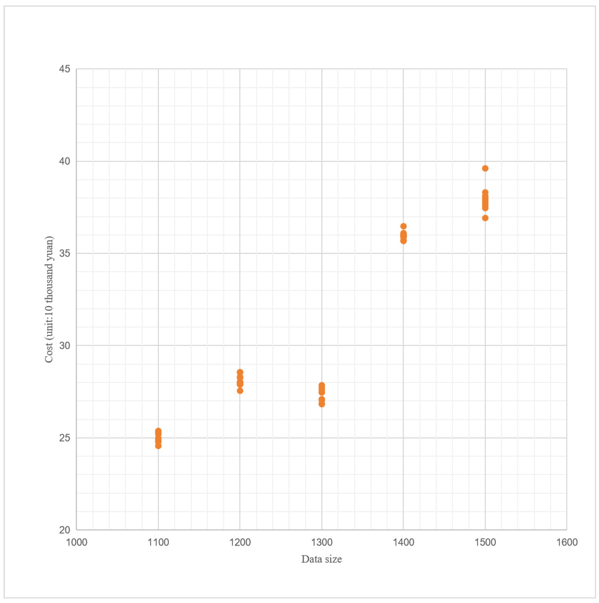
By analyzing the relationship between the cost of each data set and the data set based on the experimental results, the correlation between the cost of the optimal solution and the data set can be observed, as shown in Figure 1.

Examining

Table 7. Cost composition.

Data Set	Charging Cost	Driving Cost	Waiting Cost	Vehicle Cost	Total Cost
1200	0.38	23.27	0.46	4.14	28.25
1300	0.26	21.59	0.69	4.52	27.05
Cost Variance	−0.12	−1.68	0.23	0.38	−1.2

, it becomes apparent that the cost to solve is not linearly correlated with the size of the dataset. However, as the number of customer points increases, the cost exhibits an upward trend. Notably, the cost to solve the data set with a task point size of 1300 is generally lower than that of the dataset with a task point size of 1200, presenting an anomalous situation. Consequently, further exploration into the cost composition is conducted for experiments with customer point capacities of 1200 and 1300. This exploration utilizes the results from the first experiment of variable neighborhood search (unit: ten thousand).

Analyzing the cost structure of the two experimental results in Table 7, it is evident that an increase in the number tasks leads to higher vehicle usage costs, with the driving cost constituting the majority of the total cost. Variations in driving costs contribute to differences in total costs. It can be reasonably inferred that the lack of a strong correlation between mileage and the number of tasks is due to factors such as the spatial distribution of task points, variations in time windows, and differences in road network data. Consequently, there is no linear correlation between the cost to solve and the number of tasks.

The table data indicate that as the number of customer points increases, the vehicle utilization cost exhibits an upward trend in the solution results, contributing to an overall cost increase with more customer points. However, in the 1300 data set, the customer points are evenly distributed, and the warehouse is situated close to the center of these points. This proximity allows vehicles to efficiently serve more customers within a shorter driving distance. Consequently, this results in reduced driving and charging costs compared to the 1200 data set. Given that driving costs constitute a substantial portion of the total cost, the 1300 data set yields a smaller overall cost than its 1200-sized counterpart.

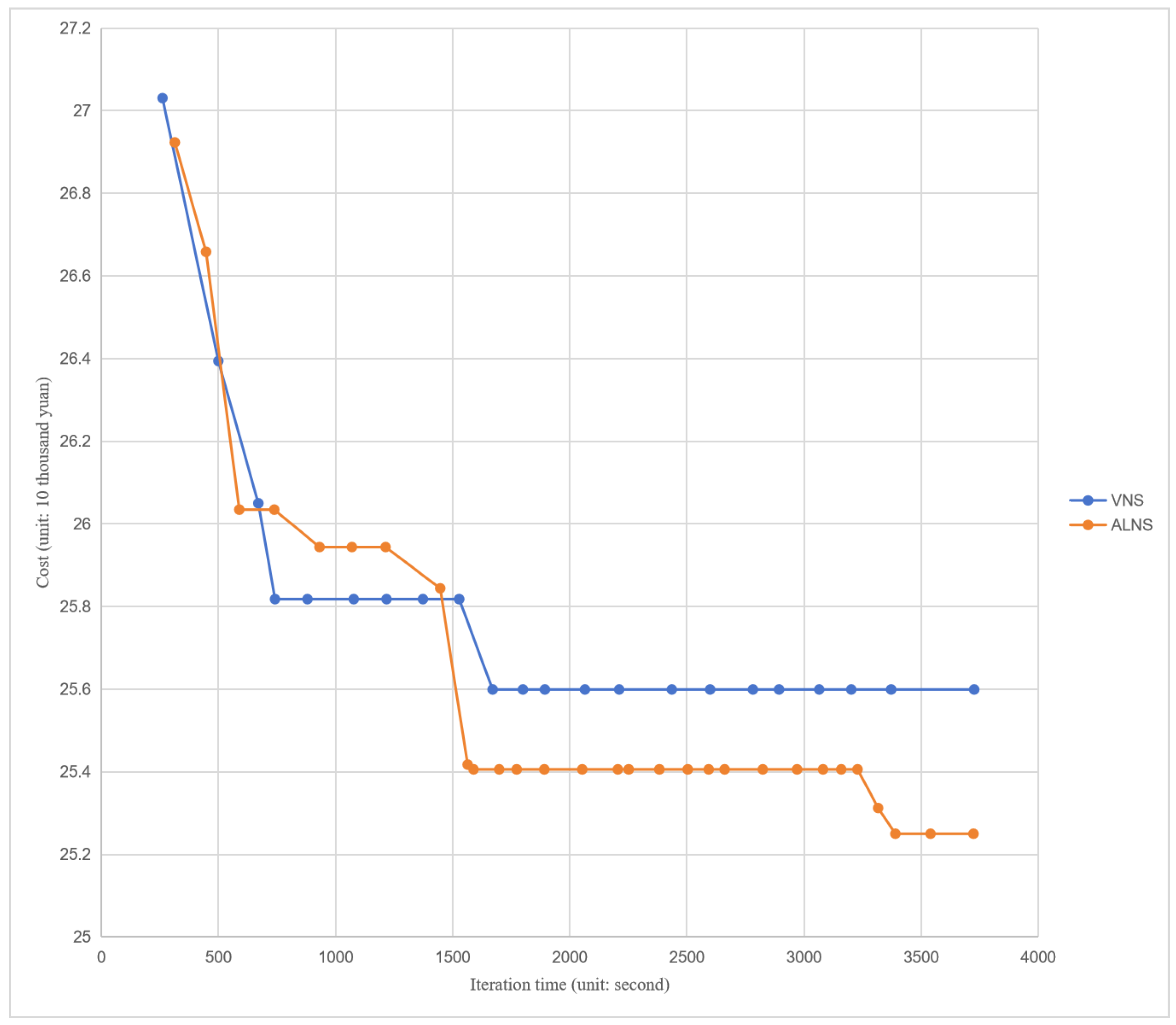
During the experiment, the completion time of each iteration was recorded. The experimental data from the adaptive large neighborhood search and variable neighborhood search for the 1100 data sets were plotted on a line chart based on the iteration time and the optimal solution cost at that time. The resulting line chart is depicted in Figure 2.

It is evident from Figure 2 that the variable neighborhood search algorithm demonstrates superior search efficiency compared to the adaptive large neighborhood search within a short timeframe. When the program’s running time is under 1500 s, the solution cost of the variable neighborhood search is lower than that of the adaptive large neighborhood search.

However, with prolonged search times, the adaptive large neighborhood search outperforms the variable neighborhood search in terms of solution results. As illustrated by the line chart, the variable neighborhood search algorithm is more prone to converging to a local optimal solution. Remarkably, the cost of the adaptive large neighborhood search continues to decrease even after 3000 s.

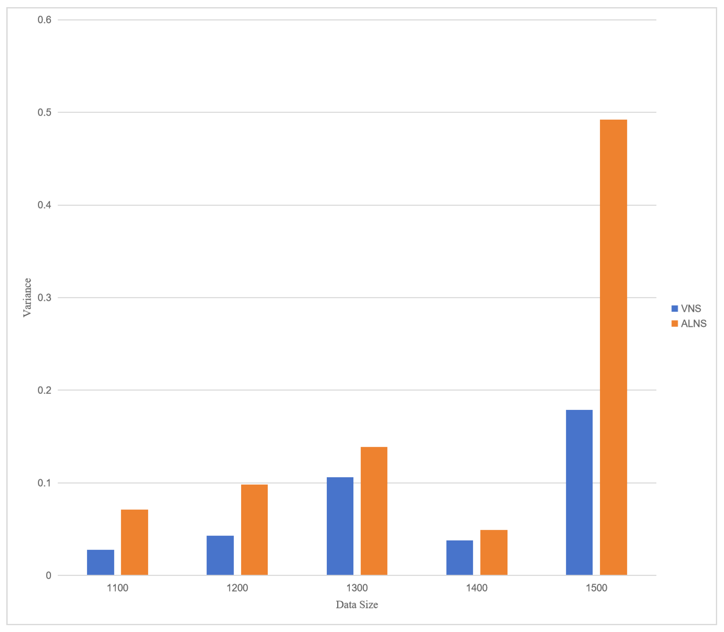
5.3.2. Analysis of Variance

We gauge the fluctuation of experimental results by calculating the variance. Figure 3 illustrates that ALNS performs least effectively on the 1500 data set, with a variance of 0.492, while its best performance is observed on the 1400 data set (0.049). The fluctuation of ALNS results is notably influenced by the inherent characteristics of the data set. Conversely, VNS exhibits better variances than ALNS across all five data sets, indicating superior stability. Moreover, the considerable variation in results between the two algorithms across different data sets emphasizes the substantial impact of data set characteristics on algorithmic performance.

Analyzing the variance in relation to the number of tasks in the data set and algorithmic results reveals no discernible correlation. This lack of correlation can be attributed to variations in time windows, geographical distribution, and road network data within the data sets.

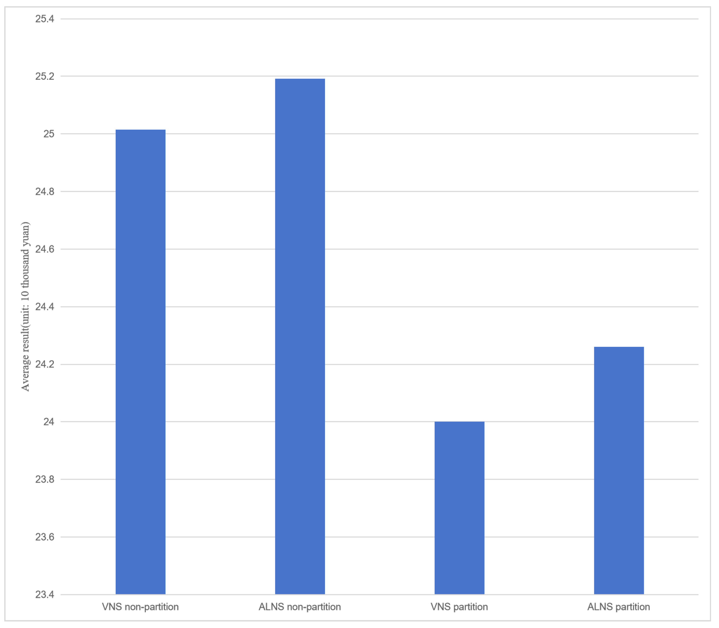
5.4. Experiments of Partition Optimization

To enhance solution efficiency, customers are grouped into multiple regions based on their geographical locations. In this section, we illustrate this approach using data sets with 1100 customers and dividing into nine regions. The comparative results between partitioned and non-partitioned scenarios are presented in Figure 4. The partition experiment demonstrates an average reduction of 3.87% in the total cost compared to the non-partitioned result, indicating a significant degree of optimization. After partitioning the data set, the objective values of VNS and ALNS decrease by 4.05% and 3.69%, respectively. The optimization level achieved through partitioning is comparable for both algorithms in this data set.

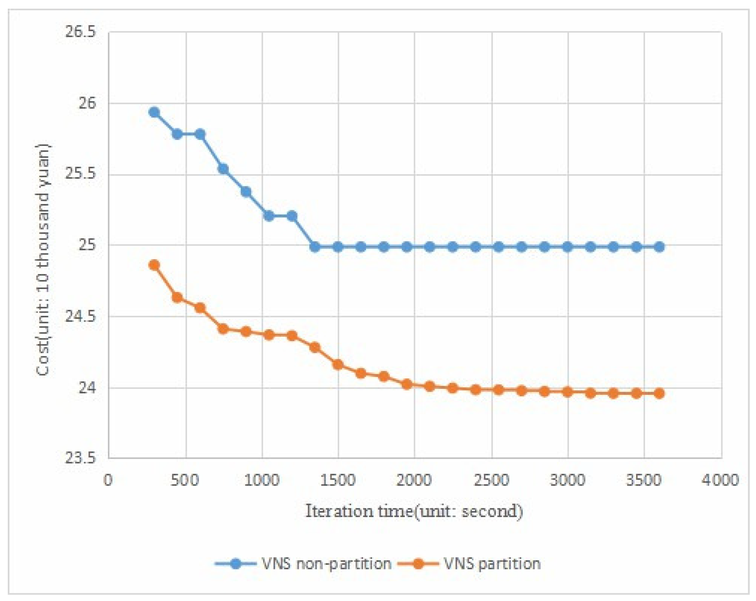
To validate solution efficiency, the correlation between the total cost and running time is depicted in Figure 5 for VNS with and without partitioning. Given the higher iterative efficiency post-partitioning, the cost of the partitioning experiment is lower than that of the non-partitioning experiment from the initial solution generation. Notably, the non-partitioning experiment becomes trapped in a local optimal solution around 1500 s. Due to its superior optimization effect compared to the non-partitioning experiment, the partitioning experiment achieves a better cost in the same timeframe.

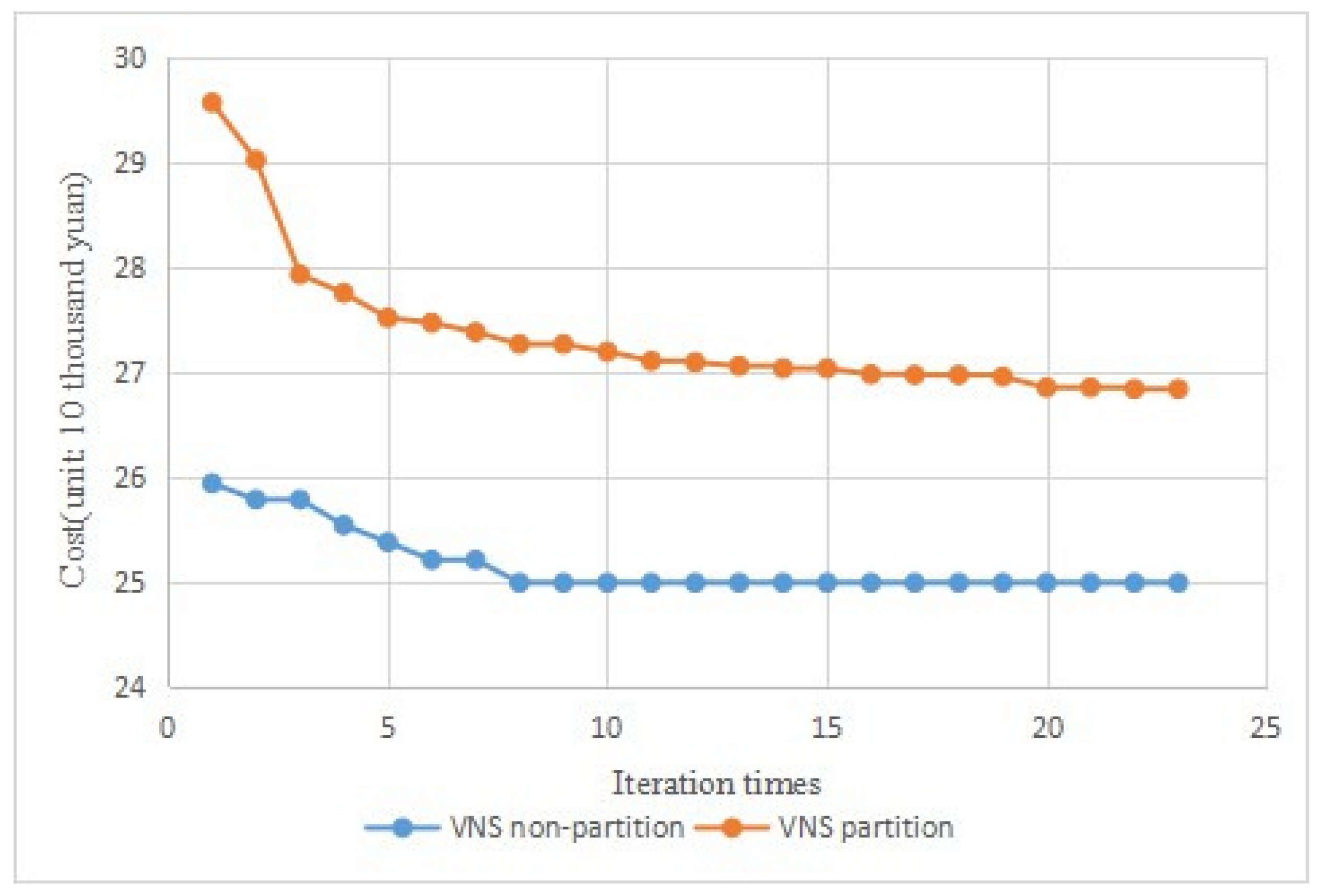
In theory, partitioned solutions, driven by local considerations rather than global ones, should avoid the global solution being more expensive. However, experimental results indicate that the outcomes of the partitioning experiment are superior to those of the global experiment. To further investigate, we control for the same number of iterations and compare the solution results of the partitioning and non-partitioning experiments, as shown in Figure 6. Interestingly, when the number of iterations is the same, the results of the non-partitioning experiment surpass those of the partitioning experiment. These experiments suggest that, despite the side effects caused by the failure of local considerations due to partitioning, the significant increase in iteration efficiency post-partitioning leads to a higher degree of optimization. When both experiments are conducted with the same number of iterations, the non-partitioned result is lower than that of the partitioned.

5.5. Sensitivity Analysis

To further assess the effectiveness of the proposed model, a sensitivity analysis was conducted on the service time and vehicle range.

5.5.1. The Customer Service Time

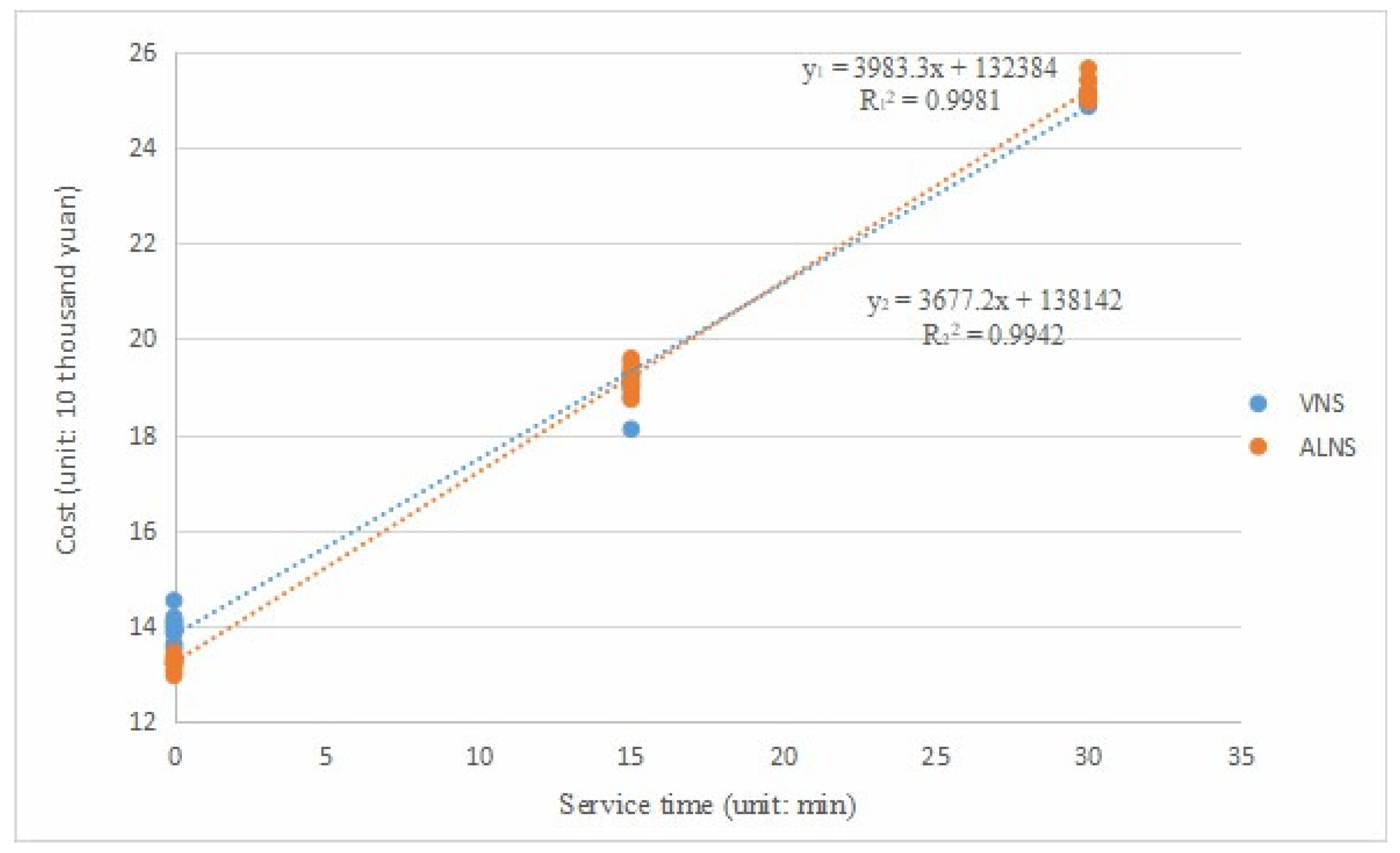
Sensitivity experiments were conducted by varying the service time by reducing it from 30 min to 15 min or 0 min. The experimental results are illustrated in Figure 7. From the scatter plot in Figure 7, it is evident that the relationship between distribution cost and customer time is nearly linear. Comparing the trajectory curves of the two algorithms, it is observed that the ALNS program is more sensitive to the reduction in customer service time, while the VNS exhibits a relatively slower response to the change in time.

5.5.2. Vehicle Range

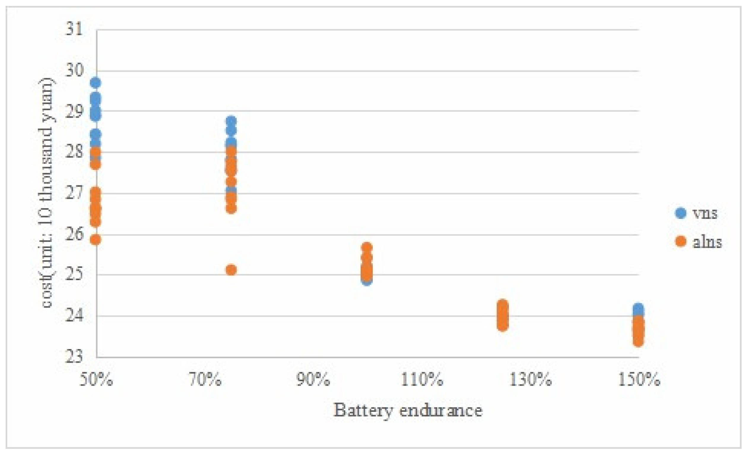
Next, the vehicle’s range is varied by an appropriate percentage, i.e., 50%, 75%, 100%, 125%, or 150%, to analyze the experimental results. The outcomes are depicted in a bar chart, as shown in Figure 8.

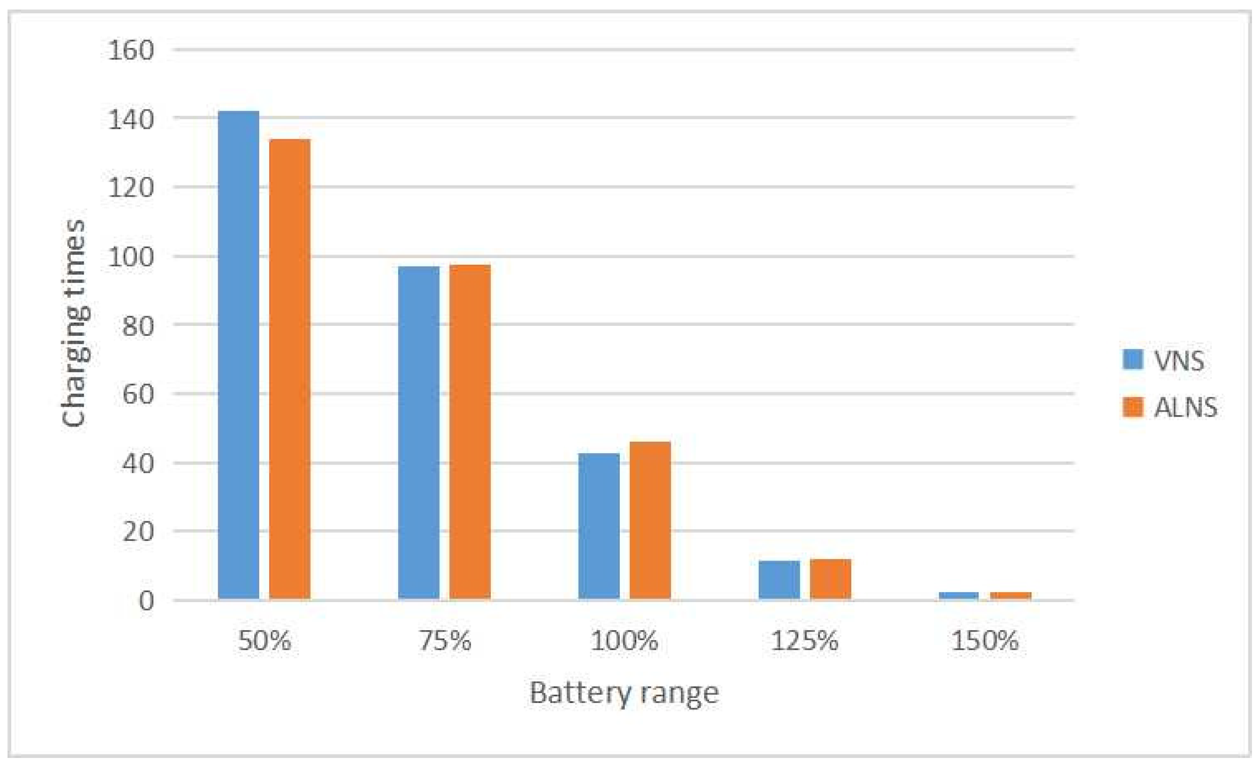
From the experimental results and data in Figure 8, it is evident that the vehicle cost increases with a reduction in the vehicle range. Conversely, as the vehicle range increases, the vehicle cost decreases relative to the original solution. However, there is no significant difference in the resulting cost between the 125% battery range and the 150% battery range. To investigate this phenomenon, the charging times of the experimental results with 125% and 150% battery quantities are statistically analyzed, and the results are presented in Figure 9.

Based on the initial assumption of the original vehicle battery range, the average number of charging times is 42.8. When the vehicle range is reduced to 75% or 50% of the original solution, the average charging times increase to 97 or 142 times, respectively. These results demonstrate that as the vehicle range decreases, the charging frequency significantly rises, leading to increased costs. Conversely, when the vehicle range is increased to 125% of the original solution, the average charging times decrease to 11.8 times, resulting in a notable reduction in costs. Further, increasing the vehicle range from 125% to 150% yields an average of 2.3 charging times, indicating a more modest reduction compared to the 125% scenario. It can be inferred that the experiment is constrained by other factors, such as time windows and service times, and the number of task points to which a vehicle can deliver is limited. Consequently, distribution costs cannot decrease indefinitely by simply extending the vehicle range.

6. Conclusions and Future Research

This paper introduces an enhanced version of the electric vehicle routing problem, known as H-MT-EVRP-PD, which incorporates multiple vehicle types with varying capacities and volumes. The problem involves vehicles performing multiple trips per day due to capacity limitations and the goal of minimizing the fleet size. Both delivery and pickup activities are considered in the context of express delivery parcels. While a mathematical programming model is presented to formally define the problem, it is noted that this model is optimal only for very small instances. To address larger real-world scenarios, two heuristic algorithms, namely VNS and ALNS, are proposed and comprehensively evaluated through computational experiments.

The primary focus of this paper revolves around the scenario and model of the problem and features two key innovations:

(1)

We introduce a novel multi-attribute multi-vehicle routing problem by integrating established problem domains, including the heterogeneous vehicle routing problem (HVRP), multi-trip vehicle routing problem (MTVRP), pickup problem for cargo transportation (PDP), and the recently formulated electric vehicle routing problem with time windows and charging stations (E-VRPTW). We formulate this amalgamation as a mixed-integer programming model (H-MT-EVRP-PD).

(2)

We propose an effective variable neighborhood search algorithm (VNS) and an adaptive large neighborhood search algorithm (ALNS) specifically designed to address the challenges posed by the problem defined in this paper. The experimental results highlight the efficiency of the developed algorithms in solving the vehicle routing problem within the proposed scenario. These findings underscore the algorithms’ effectiveness in addressing the unique challenges associated with electric vehicle logistics distribution.

By analyzing the experimental results, the following conclusions are drawn:

(1) The VNS is more efficient in the initial search stage, and thus the VNS outperforms the ALNS in conditions of high requirements for computing time. However, the ALNS is more effective in conditions for which we are expecting to obtain a lower cost and which are less sensitive to computing time. (2) For large-scale problems, H-MT-EVRP-PD can obtain a high-quality solution in the same computing time by means of partitioning: even a simple partition according to the geographical location. (3) Due to the impact of complex constraints, increasing the vehicle range cannot significantly reduce the vehicle operating cost, yet reducing customer service time can significantly reduce delivery costs.

This paper assumes that the vehicle is always recharged to full capacity, whereas it would be interesting to relax the full-recharge restriction and allow partial recharging, which is more practical in the real world (e.g., [9]). Furthermore, the travel speeds on the road might vary during peak and off-peak hours in urban areas as discussed in [1], which is also an interesting topic for future research focusing on extending our model to real-world cases. In addition, it is assumed that recharging stations are always available, whereas vehicles may need to queue at the station. Thus, considering the stochastic recharging time will be one of the subjects of future work. Simultaneously, we anticipate delving into more efficient algorithms in future studies.

References

- Pan, B.; Zhang, Z.; Lim, A. Multi-trip time-dependent vehicle routing problem with time windows. Eur. J. Oper. Res. 2021, 291, 218–231. [Google Scholar] [CrossRef]
- Sartori, C.S.; Buriol, L.S. A study on the pickup and delivery problem with time windows: Matheuristics and new instances. Comput. Oper. Res. 2020, 124, 105065. [Google Scholar] [CrossRef]
- Hiermann, G.; Puchinger, J.; Ropke, S.; Hartl, R.F. The electric fleet size and mix vehicle routing problem with time windows and recharging stations. Eur. J. Oper. Res. 2016, 252, 995–1018. [Google Scholar] [CrossRef]
- Schneider, M. The electric vehicle-routing problem with time windows and recharging stations. Transp. Sci. 2014, 48, 500–520. [Google Scholar] [CrossRef]
- Yang, J.; Sun, H. Battery swap station location-routing problem with capacitated electric vehicles. Comput. Oper. Res. 2015, 55, 217–232. [Google Scholar] [CrossRef]
- Jun, Y.; Peng-xiang, F.; Hao, S. Battery exchange station location and vehicle routing problem in electric vehicles distribution system. Chin. J. Manag. Sci. 2015, 23, 87–96. [Google Scholar]
- Gao, S. The Research of Vehicle Routing Problem with Time Window Based on Electric Vehicle. Ph.D. Thesis, Dalian Maritime University, Dalian, China, 2015. [Google Scholar]
- Wang, Y.C. Research on Vehicle Routing Problem of City Distribution Based on Pure Electric Vehicle. Master’s Thesis, Beijing Jiaotong University, Beijing, China, 2016. [Google Scholar]
- Keskin, M.; Çatay, B. Partial recharge strategies for the electric vehicle routing problem with time windows. Transp. Res. Part C Emerg. Technol. 2016, 65, 111–127. [Google Scholar] [CrossRef]
- Felipe, Á.; Ortuño, M.T.; Righini, G.; Tirado, G. A heuristic approach for the green vehicle routing problem with multiple technologies and partial recharges. Transp. Res. Part E Logist. Transp. Rev. 2014, 71, 111–128. [Google Scholar] [CrossRef]
- Montoya, A.; Guéret, C.; Mendoza, J.E.; Villegas, J.G. The electric vehicle routing problem with nonlinear charging function. Transp. Res. Part B Methodol. 2017, 103, 87–110. [Google Scholar] [CrossRef]
- Koç, Ç.; Jabali, O.; Mendoza, J.E.; Laporte, G. The electric vehicle routing problem with shared charging stations. Int. Trans. Oper. Res. 2019, 26, 1211–1243. [Google Scholar] [CrossRef]
- Toth, A.; Paolo, B.; Vigo Daniele, C. Vehicle Routing: Problems, Methods, and Applications; SIAM: Philadelphia, PA, USA, 2014. [Google Scholar]
- Stewart, W.R., Jr.; Golden, B.L. A Lagrangean relaxation heuristic for vehicle routing. Eur. J. Oper. Res. 1984, 15, 84–88. [Google Scholar] [CrossRef]
- Golden, B.L.; Raghavan, S.; Wasil, E.A. The Vehicle Routing Problem: Latest Advances and New Challenges; Springer: Berlin/Heidelberg, Germany, 2008; pp. 3–27. [Google Scholar]
- Dondo, R.; Cerdá, J. A cluster-based optimization approach for the multi-depot heterogeneous fleet vehicle routing problem with time windows. Eur. J. Oper. Res. 2007, 176, 1478–1507. [Google Scholar] [CrossRef]
- Paraskevopoulos, D.C.; Repoussis, P.P.; Tarantilis, C.D.; Ioannou, G.; Prastacos, G.P. A reactive variable neighborhood tabu search for the heterogeneous fleet vehicle routing problem with time windows. J. Heuristics 2008, 14, 425–455. [Google Scholar] [CrossRef]
- Yoshizaki, H.T. Scatter search for a real-life heterogeneous fleet vehicle routing problem with time windows and split deliveries in Brazil. Eur. J. Oper. Res. 2009, 199, 750–758. [Google Scholar]
- Jiang, J.; Ng, K.M.; Poh, K.L.; Teo, K.M. Vehicle routing problem with a heterogeneous fleet and time windows. Expert Syst. Appl. 2014, 41, 3748–3760. [Google Scholar] [CrossRef]
- Petch, R.J.; Salhi, S. A multi-phase constructive heuristic for the vehicle routing problem with multiple trips. Discret. Appl. Math. 2003, 133, 69–92. [Google Scholar] [CrossRef]
- Olivera, A.; Viera, O. Adaptive memory programming for the vehicle routing problem with multiple trips. Comput. Oper. Res. 2007, 34, 28–47. [Google Scholar] [CrossRef]
- Cattaruzza, D.; Absi, N.; Feillet, D.; Vidal, T. A memetic algorithm for the multi trip vehicle routing problem. Eur. J. Oper. Res. 2014, 236, 833–848. [Google Scholar] [CrossRef]
- Azi, N.; Gendreau, M.; Potvin, J.Y. An adaptive large neighborhood search for a vehicle routing problem with multiple routes. Comput. Oper. Res. 2014, 41, 167–173. [Google Scholar] [CrossRef]
- François, V.; Arda, Y.; Crama, Y.; Laporte, G. Large neighborhood search for multi-trip vehicle routing. Eur. J. Oper. Res. 2016, 255, 422–441. [Google Scholar] [CrossRef]
- Azi, N.; Gendreau, M.; Potvin, J.Y. An exact algorithm for a single-vehicle routing problem with time windows and multiple routes. Eur. J. Oper. Res. 2007, 178, 755–766. [Google Scholar] [CrossRef]
- Cattaruzza, D.; Absi, N.; Feillet, D. The multi-trip vehicle routing problem with time windows and release dates. Transp. Sci. 2016, 50, 676–693. [Google Scholar] [CrossRef]
- Hernandez, F.; Feillet, D.; Giroudeau, R.; Naud, O. A new exact algorithm to solve the multi-trip vehicle routing problem with time windows and limited duration. 4OR 2014, 12, 235–259. [Google Scholar] [CrossRef]
- Savelsbergh, M.W.; Sol, M. The general pickup and delivery problem. Transp. Sci. 1995, 29, 17–29. [Google Scholar] [CrossRef]
- Shang, J.S.; Cuff, C.K. Multicriteria pickup and delivery problem with transfer opportunity. Comput. Ind. Eng. 1996, 30, 631–645. [Google Scholar] [CrossRef]
- Nanry, W.P.; Barnes, J.W. Solving the pickup and delivery problem with time windows using reactive tabu search. Transp. Res. Part Methodol. 2000, 34, 107–121. [Google Scholar] [CrossRef]
- Xu, H.; Chen, Z.L.; Rajagopal, S.; Arunapuram, S. Solving a practical pickup and delivery problem. Transp. Sci. 2003, 37, 347–364. [Google Scholar] [CrossRef]
- Ropke, S.; Pisinger, D. An adaptive large neighborhood search heuristic for the pickup and delivery problem with time windows. Transp. Sci. 2006, 40, 455–472. [Google Scholar] [CrossRef]
- Baldacci, R.; Bartolini, E.; Mingozzi, A. An exact algorithm for the pickup and delivery problem with time windows. Oper. Res. 2011, 59, 414–426. [Google Scholar] [CrossRef]
- Masmoudi, M.A.; Hosny, M.; Demir, E.; Genikomsakis, K.N.; Cheikhrouhou, N. The dial-a-ride problem with electric vehicles and battery swapping stations. Transp. Res. Part E Logist. Transp. Rev. 2018, 118, 392–420. [Google Scholar] [CrossRef]
- Affi, M. General Variable Neighborhood Search Approach for Solving the Electric Two-Echelon Vehicle Routing Problem. In Proceedings of the 2020 International Multi-Conference on: “Organization of Knowledge and Advanced Technologies” (OCTA), Tunis, Tunisia, 6–8 February 2020; pp. 1–3. [Google Scholar]
- Mladenović, N.; Hansen, P. Variable neighborhood search. Comput. Oper. Res. 1997, 24, 1097–1100. [Google Scholar] [CrossRef]
- Polacek, M.; Hartl, R.F.; Doerner, K.; Reimann, M. A variable neighborhood search for the multi depot vehicle routing problem with time windows. J. Heuristics 2004, 10, 613–627. [Google Scholar] [CrossRef]
- Yao, Y.; Zhu, X.; Dong, H.; Wu, S.; Wu, H.; Tong, L.C.; Zhou, X. ADMM-based problem decomposition scheme for vehicle routing problem with time windows. Transp. Res. Part B Methodol. 2019, 129, 156–174. [Google Scholar] [CrossRef]