Obstacle Avoidance Trajectory Planning for Autonomous Vehicles on Urban Roads Based on Gaussian Pseudo-Spectral Method

Abstract

Urban autonomous vehicles on city roads are subject to various constraints when changing lanes, and commonly used trajectory planning methods struggle to describe these conditions accurately and directly. Therefore, generating accurate and adaptable trajectories is crucial for safer and more efficient trajectory planning. This study proposes an optimal control model for local path planning that integrates dynamic vehicle constraints and boundary conditions into the optimization problem’s constraint set. Using the lane-changing scenario as a basis, this study establishes environmental and collision avoidance constraints during driving and develops a performance metric that optimizes both time and turning angle. The study employs the Gauss pseudo-spectral method to continuously discretize the state and control variables, converting the optimal control problem into a nonlinear programming problem. Using numerical solutions, variable control and state trajectories that satisfy multiple constraint conditions while optimizing the performance metric are generated. The study employs two weights in the experiment to evaluate the method’s performance, and the findings demonstrate that the proposed method guarantees safe obstacle avoidance, is stable, and is computationally efficient at various interpolation points compared to the Legendre pseudo-spectral method (LPM) and the Shooting method.

1. Introduction

The reliability of active obstacle avoidance during lane-changing directly affects the safety of autonomous driving, and numerous critical issues require resolution [1,2]. Due to the vehicle system’s complexity, the variability of road environments during driving, and the requirement for real-time consideration, research on trajectory planning for autonomous driving is particularly challenging. Vehicle trajectory planning necessitates the full consideration of external environmental factors as well as the vehicle’s kinematic and dynamic constraints to design a safe driving trajectory that adheres to standard regulations while addressing comfort and stability goals. Therefore, enhancing the accuracy and reliability of trajectory planning for autonomous vehicles is an essential and challenging task. Trajectory planning for autonomous driving typically falls into four categories: curve interpolation, machine learning, sampling, and optimal control.

1.1. Sampling Method

Sampling planning methods can be broadly divided into fixed and random sampling methods. Control space sampling and state space sampling are typical fixed sampling methods. Control space sampling generates feasible kinematic trajectories by forward integrating an initial state based on control inputs. The literature [3] introduces a finite grid into the state space and obtains optimal trajectories through graph search. The target trajectory is obtained in the literature [4] by combining expected states in the horizontal and vertical state spaces with a polynomial. Typical algorithms for random sampling include Rapidly-Exploring Random Tree (RRT) and Probabilistic Roadmaps (PRM). In the literature [5], an improved RRT algorithm requires random sampling points to be generated according to a Gaussian distribution around the expected path, limits the path’s curvature, and applies three B-spline smoothing processing steps to the planned path. The RRT* algorithm was first introduced in 2010 and can significantly improve the path quality discovered in the robot’s motion space. The operation of the RRT* algorithm is very similar to that of RRT. The algorithm constructs a tree by randomly sampling in the robot’s reachable space and connects new nodes to the tree after collision and non-holonomic constraint detection. The literature [6] proposed the informed RRT* algorithm, which confines the sampling space to an elliptical area centered on the planning start and end points, with the semi-major axis of the ellipse equal to the path length. As the path length decreases, the oval area shrinks. Although sampling methods have fast computation speeds, they may need more accuracy since they determine the driving path through continuous filtering and updating. Sampling methods may not cover complex constraints and conditions. Random sampling needs motion planning tasks that do not include complex constraint conditions and do not require high solution accuracy. Global path planning is more suitable for actual road environments, considering the complexity of the environment, including constraints such as road conditions, obstacles, and vehicle dynamics.

1.2. Curve Interpolation Method

The curve interpolation method generates a smooth curve to fit the driving path by combining various curve interpolation methods. This method selects key nodes, fits multiple sets of curves based on the selected nodes, and selects a suitable curve as the optimized path according to the specific requirements of the problem. Common curve types include polynomial curves, bi-arc curves, sine function curves, Bezier curves, B-spline curves, and more. Werling et al. established a Frenet coordinate system based on the road, decomposed the motion of uncrewed vehicles into longitudinal and lateral motion, established fifth-order polynomial equations for mileage time, considered obstacle avoidance constraints, comfort factors, long-term motion modes, and outputted the optimal motion control combined with the initial and final motion states [7]. Elbanhawi et al. proposed a combination of B-spline curves and RRT, using B-spline curves’ high smoothness to reduce the search dimension and quickly generate a curvature-continuous curve suitable for wheeled robots [8]. Han et al. integrated the global path and obstacle influence in the local grid map to determine the control points, generated a collision-free fourth-order Bezier curve as the local path, and used a PID controller according to the curve [9]. A PID controller is a commonly used feedback controller used to regulate the output of a control system to achieve the desired state or value. PID stands for Proportional, Integral, and Derivative, which describe how the controller responds to error signals to adjust the output. The curve interpolation method has the advantages of fast path generation, path smoothness, and feasibility. However, a single curve function cannot fully represent the vehicle’s kinematic/dynamic equation, so interpolation polynomials are usually combined with various algorithms to plan the path.

1.3. Machine Learning

Machine learning in vehicle motion planning involves including driving task requirements, vehicle state parameters, and environmental factors in the input and output layers representing the vehicle’s projected trajectory. Machine learning techniques are employed to establish inherent connectivity through training input-output samples and then applying the trained model to real-world scenarios. Qian et al. have proposed an adaptive fuzzy neural network algorithm using combined neural networks and fuzzy reasoning, which, when applied to robot path planning, has achieved good trajectory planning performance in non-structured environments [10]. Similarly, Chen has introduced a new motion planning framework that trains a combined convolutional neural network and extended short-term memory network model, enabled by end-to-end decision-making, using accurate and virtual driving scene data [11]. It is vital to screen the quality of the data samples used in machine learning-based motion planning since the samples currently record skilled driving behavior, limiting their ability to surpass human drivers.

The nonlinearity and coupling of the vehicle itself are among the main challenges involved in trajectory planning, and striking a balance between speed and accuracy is crucial. Prioritizing speed over accuracy by simplifying vehicle modeling may prove ineffective in complex scenarios.

1.4. Optimum Control

In recent years, optimal control has gradually been applied in fields such as aerospace [12,13,14], transportation [15], and chemical industry [16]. The trajectory planning of aircraft and vehicles is the most widely used area of optimal control. In vehicle trajectory planning, many problems can be regarded as optimal control problems to solve the low precision of trajectory planning while making the computing speed as fast as possible. Therefore, it is necessary to study trajectory planning in lane change scenarios. The optimal control method consists of two essential components: the accurate establishment of the problem model and the high real-time solution method. Ren et al. improved the Newton optimization method for continuous potential field navigation models to address problems such as oscillation. They considered the effects of non-holonomic constraints and moving obstacles on robots, significantly improving system performance. However, the optimization computation cost is high [17]. Ratliff et al. propose the CHOMP (Covariant et al. Motion Planning) algorithm for high-dimensional motion planning problems. The initial path is first created from the starting to the end position. Then, the trajectory is optimized using gradient descent for the cost function, resulting in a smooth, collision-free trajectory. However, it is prone to falling into local minima, so the Hamilton Monte Carlo algorithm adds perturbations and restarts the optimization process. This method introduces randomness and reduces the certainty of the optimization results. Kalakrishnan et al. propose the STOMP (Stochastic et al. Motion Planning) algorithm, which does not require gradient information about the cost function and can improve the performance of robot motion planning. In addition, lower-cost trajectories can be obtained by generating noisy trajectories to explore the space around the initial trajectory. Its randomness also overcomes the problem of local minima in gradient-based methods [18]. Hybrid A* is a path-planning algorithm used to find the optimal path for moving objects such as vehicles or robots in continuous space. It combines A* search algorithm and a continuous space motion model to handle the motion constraints of dynamic entities such as robots or vehicles. The A algorithm is a commonly used discrete space path planning algorithm, but it is limited to handling moving objects in continuous space. Hybrid A overcomes this limitation by dividing the continuous space into discrete grids and combining them with heuristic search algorithms such as A*. It uses the vehicle’s motion model and discrete grid to search for the optimal path, while considering the vehicle’s dynamic constraints and motion in continuous space. The advantage of Hybrid A* is that it can handle motion constraints in continuous space and generate optimal paths suitable for entities such as robots or vehicles. Dolgov et al. use the Hybrid A* to generate the initial path, which aims to minimize path curvature and use the conjugate gradient method to optimize the smooth path, ensuring the safety and reliability of the path by re-optimizing the original path points that correspond to collisions [19].

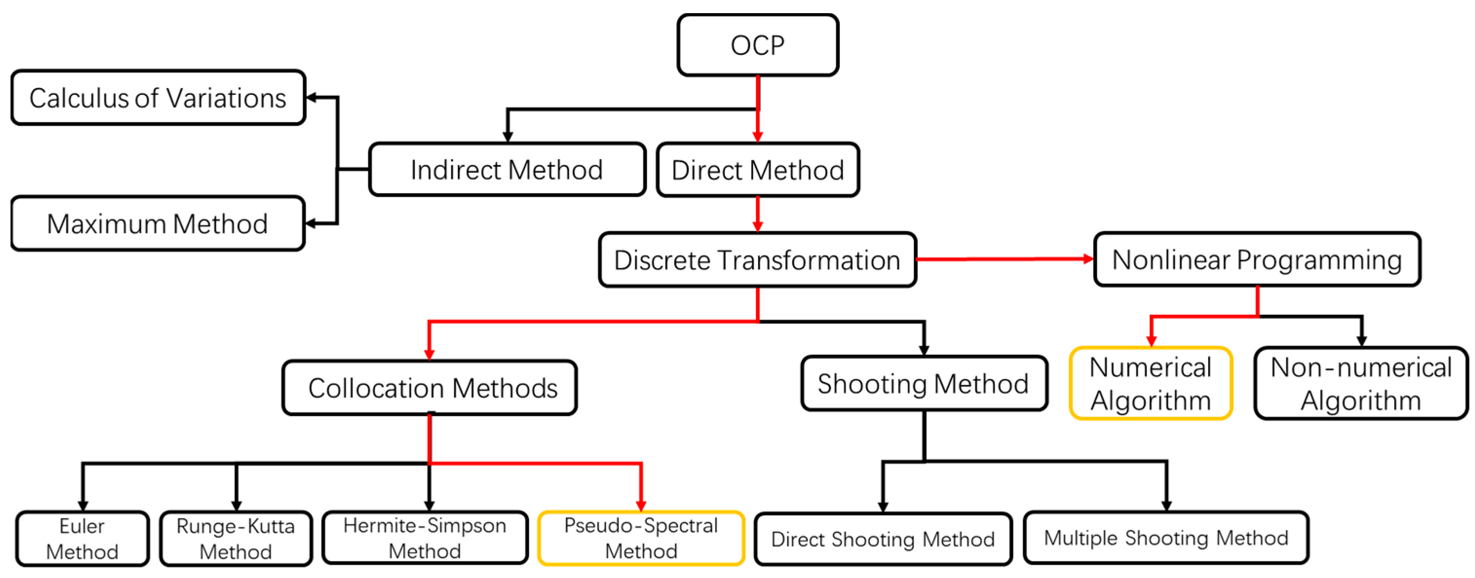
The optimal control pseudo-spectral method utilizes polynomial approximation to provide a precise numerical solution. Accurate optimization results can be obtained by selecting appropriate pseudo-spectral points. The pseudo-spectral method exhibits excellent numerical stability, effectively addressing nonlinear problems and avoiding the numerical instability and convergence difficulties frequently associated with traditional optimization methods. This approach is beneficial in optimizing trajectories for autonomous driving on urban roads while simultaneously enabling the establishment of various constraints on the vehicle’s operating state to achieve global optimization in path planning for each stage.

1.5. Contribution

(1) A performance indicator function was developed based on dual criteria—minimizing time and turning angle to address comfort and safety. Its weight was modifiable depending on the decision-making end.

(2) Incorporating the minimum safe distance of mobileye RSS to the collision avoidance restraint effectively controls surpassing the minimum safe distance.

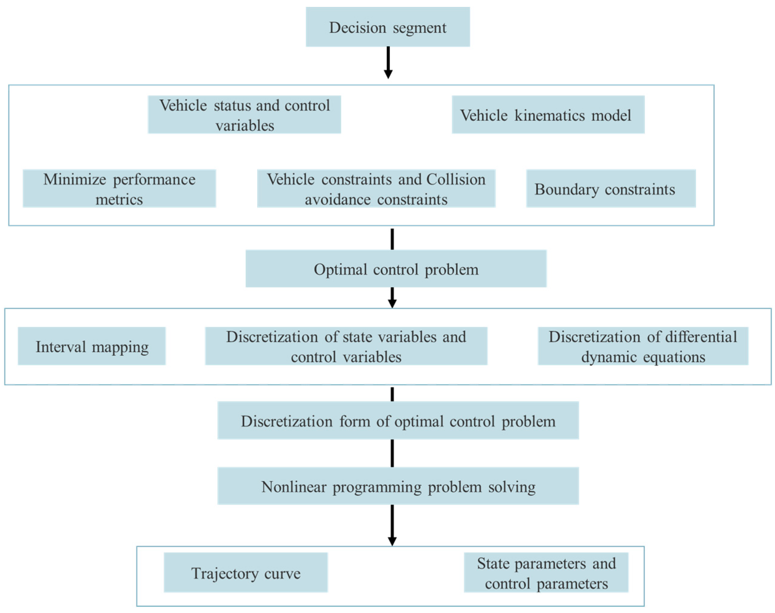
(3) The Gauss pseudo-spectral method was applied to convert the constraints and boundary conditions in the lane change process to a discrete format, simplifying the optimal control to a nonlinear programming problem.

1.6. Structure

Chapter 1: Overview of trajectory planning and its existing challenges before proposing an appropriate method.

Chapter 2: Formulates a continuous optimal control problem with vehicle, state, and road constraints that satisfy specific performance indicators.

Chapter 3: Employs the Gaussian pseudo-spectral approach within the direct method to discretize the state and control variables. With the numerical solution methods, this approach transforms the original problem into a nonlinear programming problem to acquire control variables and state trajectories that comply with various constraints while achieving optimal performance.

Chapter 4: Two weights were selected for simulation experiments and compared with the speed of LPM and DSSSM.

2. Optimal Control Model for Urban Road Autonomous Driving Path Planning

When performing driving tasks, vehicles must meet two fundamental conditions. Firstly, vehicles must travel from an initial position to a final position. Secondly, passenger comfort must be prioritized while ensuring safety. Vehicles traveling on urban roads often face congested road sections. Therefore, precise vehicle modeling proves useful for establishing optimal control models. Following vehicle modeling, constructing a path constraint system is necessary for optimal control of collision avoidance constraints. This system requires careful consideration of passenger comfort and the shortest travel times by minimizing performance indexes. The boundary constraint conditions are determined based on the initial and final positions.

2.1. An Optimal Control Model for Local Path Planning

Optimal control theory is a critical methodology in path planning. This approach models a vehicle’s motion state with differential equations, which account for kinematic principles. These differential equations incorporate motion constraints and specific performance indicators, resulting in a classical optimal control problem. Vehicle trajectory planning offers advantageous features, such as precision, directness, comprehensiveness, and completeness, by utilizing optimal control methodology.

Optimal control theory categorizes performance indexes into three types: Bolza, Mayer, and Lagrange. The Mayer type performance index is: $J=\Phi (x(t_0),t,x(t_f),t_f)$ Referred to as a constant type performance index, the Lagrange type performance index is: $J={\displaystyle {\int }_{t_0}^{t_f}L(x(t),u(t),d)dt}$.

The Bolza-type performance index represents a composite performance index in optimal control theory. It combines the Mayer constant-type performance index with the Lagrange integral-type performance index. It emphasizes both the terminal system state and the requirements during the control system process. With vehicle trajectory planning imposing constraints not only on the initial and final positions but on the entire controlled process, this study adopts the Bolza-type performance index, described as follows:

$$J=\Phi (x(t_0),t,x(t_f),t_f)+{\displaystyle {\int }_{t_0}^{t_f}L(x(t),u(t),d)dt}$$

(1)

The functional $J$ is minimized along the state trajectory line. The state trajectory is subject to constraints that limit its range; these limits arise due to the following:

Control system differential equation constraints: These differential equations encompass the vehicle’s dynamic behavior while imposing limits on its motion. Once the vehicle’s initial state and control inputs for the entire duration of movement are determined, a unique system motion can be established at any given time. The mathematical formulation is as follows:

$$\frac{dx(t)}{dt}=f(x(t),u(t),t)$$

(2)

Path constraints define the boundaries that restrict the movement of a vehicle within a particular time range. These limitations are based on specifications unique to the vehicle and factors that prevent collisions. Mathematically, the formulation of path constraints can be expressed as:

$$C(x(t),u(t),t)\le 0,t\in [t_0,t_f]$$

(3)

Boundary constraints refer to limitations on information concerning the initial and final states of the vehicle. Mathematically, it can be expressed as follows:

$$\phi (t_0,t_f,x(t_0),x(t_f),u(t_0),u(t_f))=0$$

(4)

In path constraints, $t\in [t_0,t_f]$ refers to being controlled throughout the entire planning time period.

2.2. Modeling the Kinematics of a Vehicle

The dynamic process of ground vehicle travel is complex. The vehicle model can be described with varying degrees of freedom. Greater degrees of freedom allows for a more precise vehicle model but increase the computational load. Road travel does not demand the same level of precision as parking. Hence, a two-degree-of-freedom model suffices to simulate a realistic vehicle. Thus, this paper adopts a two-degree-of-freedom vehicle kinematic model to simulate vehicle motion. The following assumptions are made when conducting vehicle kinematic modeling:

(1)

The vehicle travels on a flat road with a road surface slope is 0.

(2)

The left and right wheels have equal inclination angles, while the rear wheel’s turning angle is always 0.

(3)

The vehicle is rigid without suspension structure considerations, and the tires are always in contact with the ground at a vertical angle.

(4)

Longitudinal and lateral aerodynamics of the vehicle are ignored.

(5)

The wheels have excellent rolling contact with the ground.

A two-degree-of-freedom model is used, which combines the two front wheels and two rear wheels into a bicycle model, with its centerline as the reference, as shown in the Figure 1 below.

The differential equation is:

$$\left\{\begin{array}{l}\frac{dx(t)}{dt}=v(t)\cdot \cos \theta (t)\\ \frac{dy(t)}{dt}=v(t)\cdot \sin \theta (t)\\ \frac{d\Phi (t)}{dt}=w(t)\\ \frac{d\theta (t)}{dt}=v(t)\cdot \frac{\tan \Phi (t)}{L}\\ \frac{dv(t)}{dt}=a(t)\end{array}\right.,t\in [t_0,t_f]$$

(5)

In the Formula (5), $t_0$ is the initial time, $t_f$ is the final time, the coordinate point $(x,y)$ of the vehicle is the position of the rear wheel center of the bicycle model, $v(t)$ is the speed of the vehicle along its axial direction, $a(t)$ is the linear acceleration, $\theta (t)$ is the vehicle heading angle, that is, the angle between the x-axis in the coordinate system and the vehicle’s longitudinal center line, $\Phi (t)$ is the front wheel steering angle, with left turn being positive $w(t)$ is the front wheel steering angle velocity, $L$ represents the distance between the front and rear axles, $L_f$ represents the front overhang distance of the vehicle, $L_r$ represents the rear overhang distance, and $L_b$ represents the vehicle width.

The state variables are: $x(t)$, $y(t)$, $\Phi (t)$, $\theta (t)$, $v(t)$ are state variables $z(t)$, while $a(t)$ and $w(t)$ are control variables $u(t)$.

If the initial motion state $z(t)$ of the vehicle and the motion control $u(t)$ during the entire lane change and obstacle avoidance time $t$ are given, the vehicle’s trajectory and state during the entire time period can be determined.

2.3. Minimized Performance Metric

In the preceding section, we introduced a composite performance index of the Bolza type that incorporates a combined integral performance index of the Mayer constant value type and the Lagrange integral type, respectively. Here, the constant value performance index can be defined as time-optimal, with a weight of ${\lambda }_1$. The integral performance index can be defined as the minimum yaw angle of the vehicle, with a weight of ${\lambda }_2$, which can reflect the vehicle’s comfort during lane-changing. Minimizing the performance index requires considering the weight of both factors, which can be expressed as:

$$J={\lambda }_1\Phi (x(t_0),t,x(t_f),t_f)+{\lambda }_2{\displaystyle {\int }_{t_0}^{t_f}L(x(t),u(t),d)dt}$$

(6)

2.4. Vehicle and Collision Avoidance Constraints

The term “Vehicle constraint” refers to the limitations that are self-imposed by an autonomous vehicle during its movement. Meanwhile, the term “collision avoidance constraint” pertains to the limitations imposed where a vehicle has to steer clear of other vehicles during obstacle avoidance maneuvers.

2.4.1. Ego Vehicle Constraint

Vehicles are inherently subjected to self-restraint while driving due to their limited state and control.

$$\begin{array}{l}{v}_i(t)\le v_{\max }\\ \left|a_i(t)\right|\le a_{\max }\\ \left|{\phi }_i(t)\right|\le {\Phi }_{\max }\\ w_i(t)\le w_{\max }\end{array}$$

(7)

The formula assumes the absence of reversing situations for a vehicle, resulting in $v_i(t)$ and $w_i(t)$ being positive. Moreover, $v_{\max }$ on an urban road the highest speed a car can drive that is impacted by traffic rules, road conditions, and comfort. In addition, $a_{\max }$ is the longitudinal acceleration while $w_{\max }$ refers to the front wheel’s steering angular velocity and ${\Phi }_{\max }$ is the highest allowable front wheel steering angle.

2.4.2. Avoidance Constraint

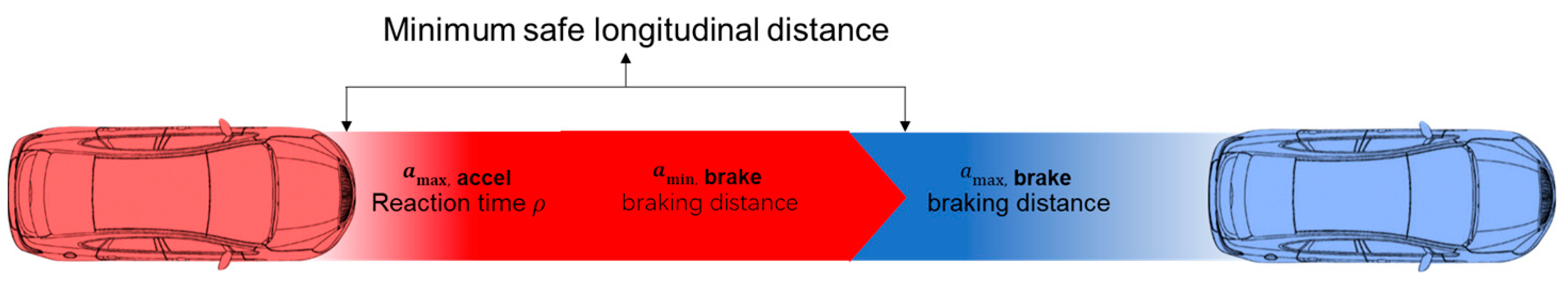
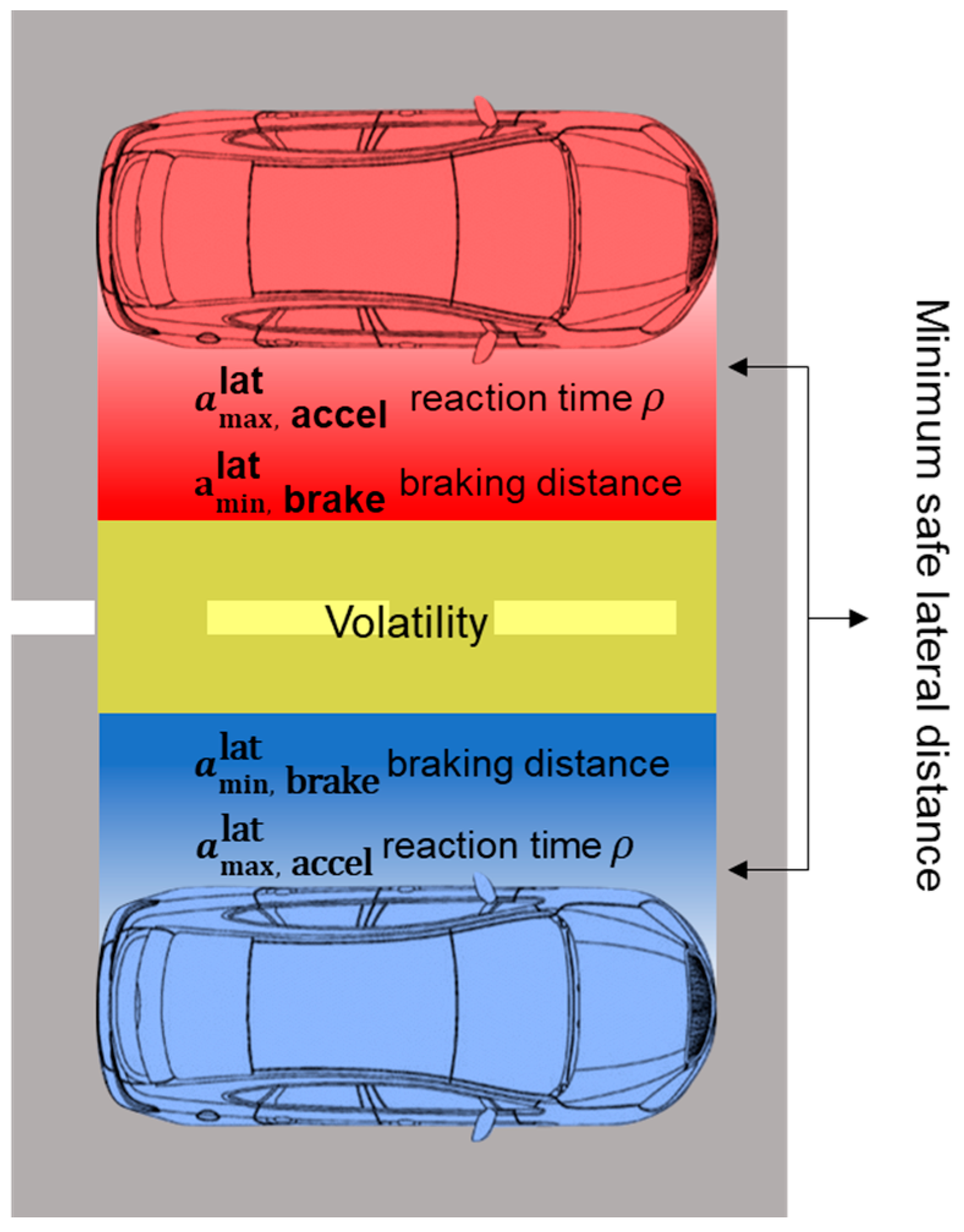
Autonomous vehicles need to avoid collisions during the entire time frame; hence, proper collision avoidance constraints must be developed. The lower speeds in urban road scenarios necessitate precise vehicle outline descriptions, and in this paper, a rectangle represents the vehicle outline model. Merely defining avoidance constraints as non-collisions is unsuitable since conflicted vehicles include not only autonomous vehicles but also driver-operated ones. An adequate space allowance should be provided to offer reaction time for conflicting vehicles. The mobileye RSS (Responsibility-Sensitive Safety) model includes a minimum safe distance calculation formula and lane change functionality. As shown in the following Figure 2 and Figure 3.

$$d_{\min ,Lo}={[v_r\rho +\frac{1}{2}{a}_{\max ,accel}{\rho }^2+\frac{{(v_r+\rho a_{\max ,accel})}^2}{2a_{\min ,brake}}-\frac{v_f^2}{2a_{\max ,brake}}]}_{+}$$

(8)

Parameter: $v_f$ is the speed of the front vehicle, $v_r$ is the speed of the rear vehicle, $\rho$ is the reaction time, $a_{\min ,brake}$ is the minimum braking acceleration, $a_{\max ,brake}$ is the maximum braking acceleration, and $a_{\max ,accel}$ is the maximum acceleration. The above formula is explained as follows:

The parameters of human drivers and autonomous vehicles are different because autonomous vehicles have a shorter reaction time. When the human driver brakes, there will be a braking reaction time, but in the case of autonomous vehicle, the braking reaction time is short. Therefore, different parameters have to be set for each of them.

$$d_{\min ,La}=\mu +{[\frac{v_1+v_{1,\rho }}{2}\rho +\frac{v_{1,\rho }^2}{2a_{\min ,brake}^{lat}}-(\frac{v_2+v_{2,\rho }}{2}\rho -\frac{v_{2,\rho }^2}{2a_{\min ,brake}^{lat}})]}_{+}$$

(9)

According to Figure 2 and Figure 3, parameter explanation: $a_{\min ,brake}^{lat}$ is the minimum lateral braking acceleration. During the lane-changing process, a certain lateral margin is given to provide lateral vehicles with sufficient reaction time, allowing for enough distance to brake and avoid collisions as much as possible.

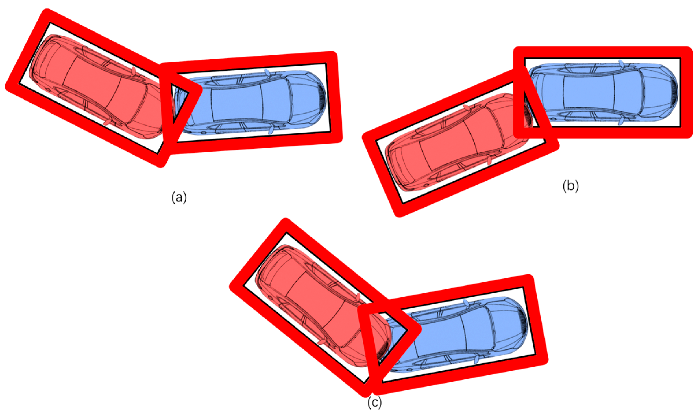
Rectangles describe the vehicle contour and incorporate the design of lateral and longitudinal safety distances of the RSS. Firstly, collision avoidance constraints between vehicles are established. The minimum values for $d_{\min ,La}$ and $d_{\min ,Lo}$ safety distances are added to the vehicle outlines if the simplified rectangle frames of two vehicles do not overlap, indicating they are not colliding. If vehicle a’s endpoint is within vehicle b’s bounds, or at least one of vehicle b’s endpoints is within vehicle a’s bounds, a collision is deemed to have occurred. As shown in the following Figure 4 and Figure 5.

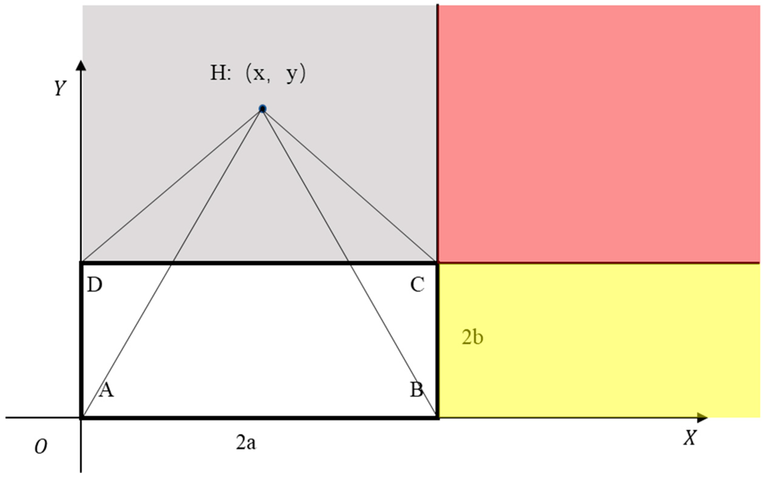
To prevent collisions, all four vertices of each rectangle should be located outside of the contour. Constraints are leveraged on the eight vertices of both contours while area-based inequalities are utilized to gauge the vertices’ whereabouts about the contour.

According to Figure 4 and Figure 5, establish a coordinate system with point $A$ as the origin in a counterclockwise direction labeled as $A$, $B$, $C$, and $D$. Assuming point H lies outside the outline, the rectangle has a length of $2a$ and a width of $2b$. Extending $DC$ and $BC$ divides the region into gray, red, and yellow zones. Using the first quadrant as an example, when $H$ is in the gray zone:

$$\begin{array}{c}0\le x\le 2a\\ y\ge 2b\end{array}$$

(10)

$S_{HAB}=2ay$, $S_{HBC}=b\times (2a-x)$, $S_{HCD}=a\times (y-2b)$, $S_{HDA}=bx$, $S_{ABCD}=4ab$, The following conclusions are drawn:

$$S_{HAB}+S_{HBC}+S_{HCD}+S_{HDA}>S_{ABCD}$$

(11)

Similarly, the same rule applies to the red and yellow zones, as well as the second, third, and fourth quadrants. Consequently, the formula mentioned above can be employed to determine the relative position of vertices to the rectangle.

Below is a model for the vehicle collision constraints: The vehicle’s rectangular contour is defined by $ABCD$ according to the vertex sequence as earlier described. $D$ and $A$ denote the left-front and right-rear sides of the vehicle, respectively. The coordinates are determined based on the vehicle’s structural relationship, yielding the following results:

$$\begin{array}{c}A=(A_x,A_y)=[x-(L_r+d_{\min ,Lo})\cdot \cos \theta +0.5(L_b+d_{\min ,La})\cdot \sin \theta ,\\ y-(L_r+d_{\min ,La})\cdot \sin \theta -0.5(L_b+d_{\min ,La})\cos \theta ]\\ B=(B_x,B_y)=\{[x+(L+L_{\mathrm{f}}+d_{\min ,Lo})]\cdot \cos \theta +0.5(L_b+d_{\min ,La})\cdot \sin \theta ,\\ y+(L+L_f+d_{\min ,Lo})\cdot \sin \theta -(0.5L_b+d_{\min ,La})\cdot \cos \theta ]\}\\ C=(C_x,C_y)=\{[x+(L+L_{\mathrm{f}}+d_{\min ,Lo})]\cdot \cos \theta -0.5(L_b+d_{\min ,La})\cdot \sin \theta ,\\ y+(L+L_f+d_{\min ,Lo})\cdot \sin \theta +(0.5L_b+d_{\min ,La})\cdot \cos \theta ]\}\\ D=(D_x,D_y)=[x-(L_r+d_{\min ,Lo})\cdot \cos \theta -0.5(L_b+d_{\min ,La})\cdot \sin \theta ,\\ y-(L_r+d_{\min ,La})\cdot \sin \theta +0.5(L_b+d_{\min ,La})\cdot \cos \theta ]\end{array}$$

(12)

In the vehicle position relationship, the state variables $x$, $y$, and $\theta$ are all functions of time $t$. This means that the vehicle contour coordinate values can be determined using the formulas mentioned above at every time interval. Therefore, the collision constraints for vehicles $a$ and $b$ are:

$$\left\{\begin{array}{l}{S}_{M{A}_a{B}_a}+S_{M{B}_a{C}_a}+S_{M{C}_a{D}_a}+S_{M{D}_a{A}_a}\ge S_{A_a{B}_a{C}_a{D}_a},M\in \left\{A_b{B}_b{C}_b{D}_b\right\}\\ S_{N{A}_b{B}_b}+S_{N{B}_b{C}_b}+S_{N{C}_b{D}_b}+S_{N{D}_b{A}_b}\ge S_{A_b{B}_b{C}_b{D}_b},M\in \left\{A_a{B}_a{C}_a{D}_a\right\}\end{array}\right.$$

(13)

The $S_{A_a{B}_a{C}_a{D}_a}$ and $S_{A_b{B}_b{C}_b{D}_b}$ are the rectangular areas of car $a$ and car $b$ themselves, respectively. The areas are $(L_r+L_f+L+d_{\min ,Lo})\times (L_b+d_{\min ,La})$.

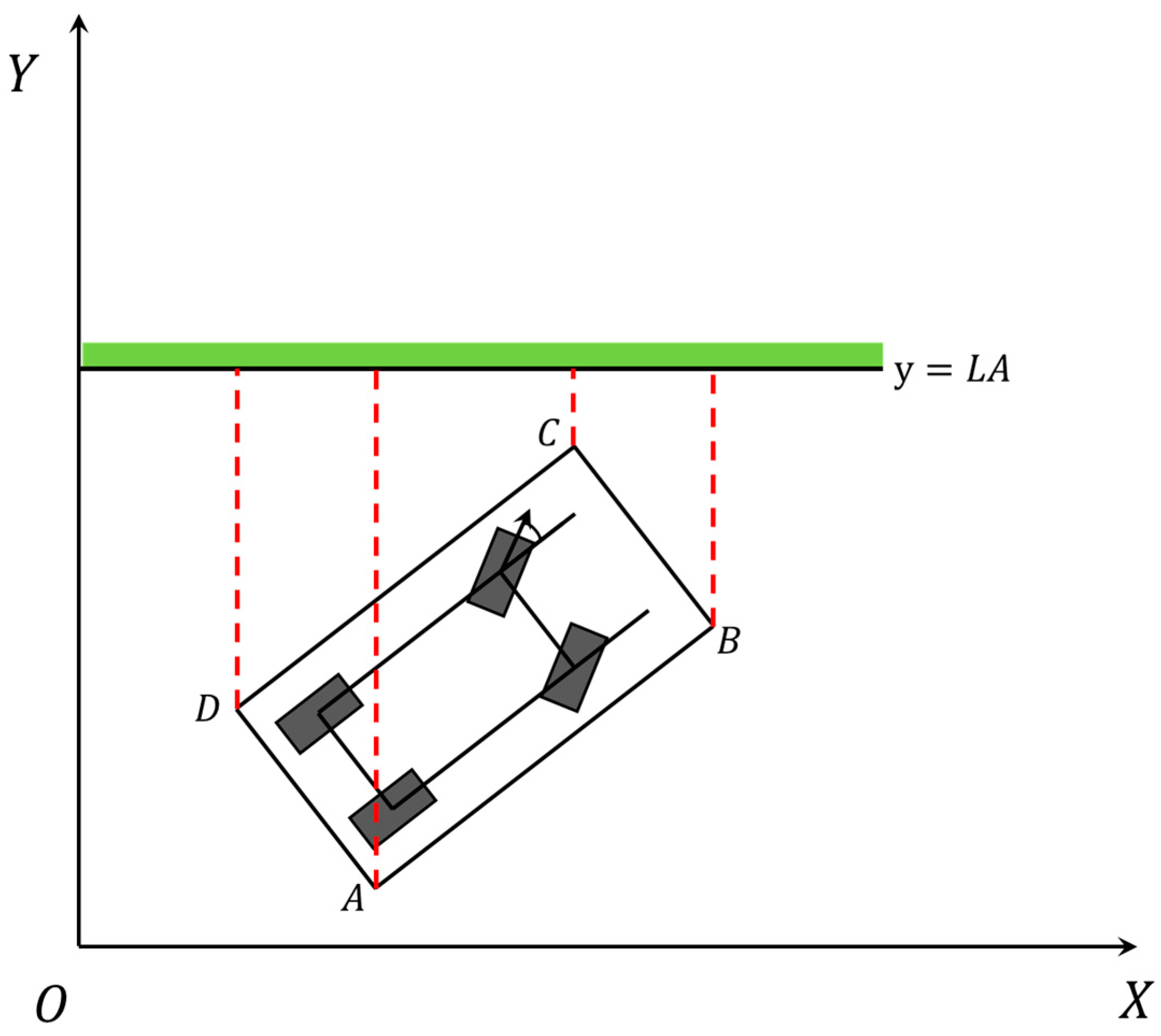
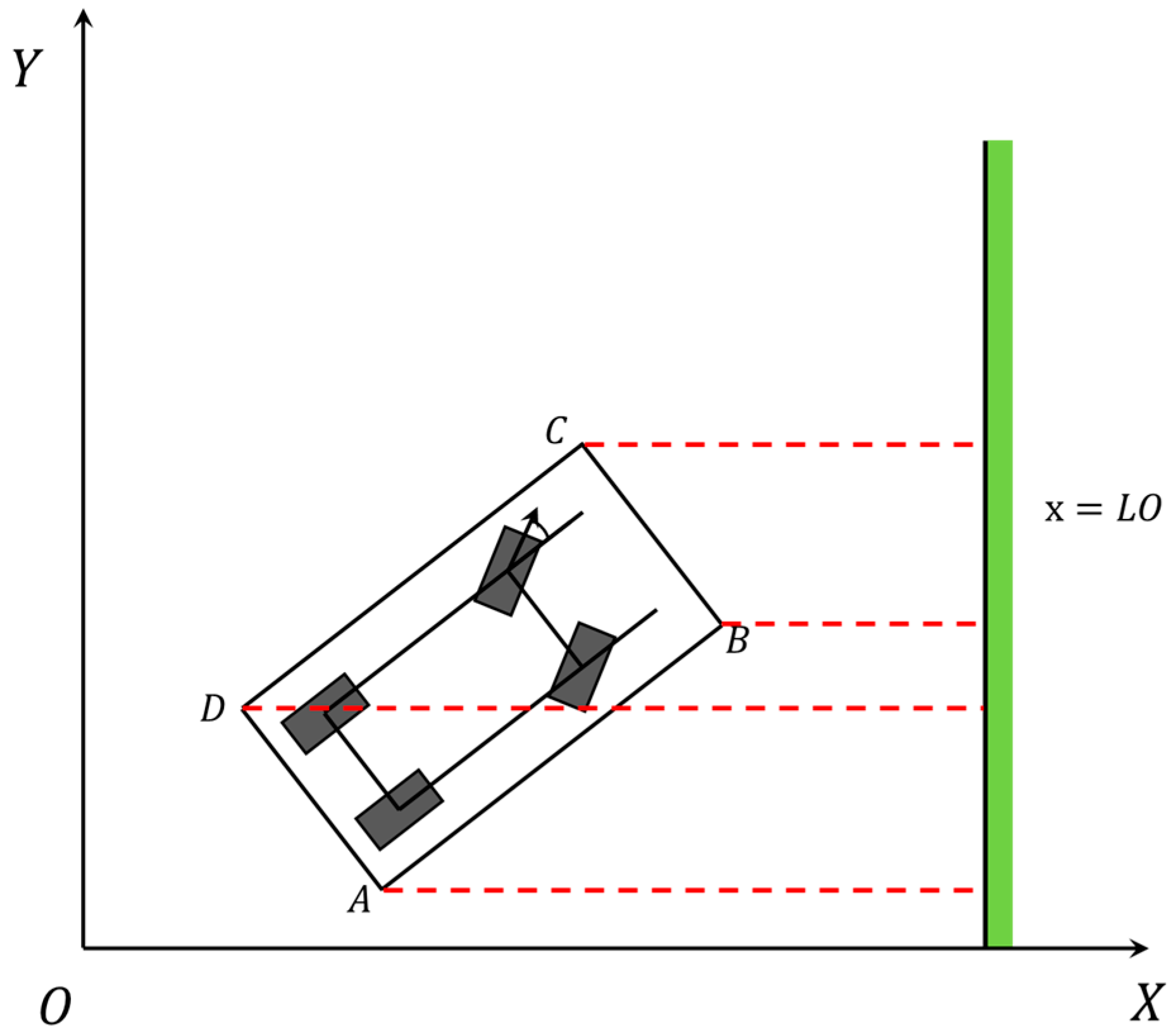
During the collision avoidance process, while avoiding obstacles between vehicles, it is also necessary to consider avoiding collisions with the edge of the road, and the vehicle frame line does not collide with the edge. When the vehicle boundary does not collide with the edge, it is equivalent to the boundary always remaining on the side of the road edge between $t_0$ and $t_f$ without crossing the edge line. As shown in the following Figure 6 and Figure 7.

The vehicle and the road edge have a constant value of $y=LA$:

$$P\le LA,P\in \{A_y(t),B_y(t),C_y(t),D_y(t)\},t\in [t_0,t_f]$$

(14)

When $T$ is equal to 1.

The vehicle and the road edge have a constant value of $x=LO$:

$$P\le LO,P\in \{A_x(t),B_x(t),C_x(t),D_x(t)\},t\in [t_0,t_f]$$

(15)

2.5. Boundary Constraint

Boundary constraints on the state variable $x(t)$ and control variable $u(t)$ exist at the initial and final times, $t_0$ and $t_f$, respectively, during the vehicle’s motion. Thus, it is essential to establish the actual boundary conditions.

At the beginning, $t=t_0$ and end $t=t_f$ times of the vehicle’s motion, the following state and control variables are considered first:

$$[a(t_0),w(t_0),v(t_0),\Phi (t_0),\theta (t_0),x(t_0),y(t_0)]=[a,w,v,\Phi ,\theta ,x,y]$$

(16)

Initially, to satisfy the boundary constraints at the beginning and end of the vehicle’s motion, the vehicle must have an initial zero relative velocity and zero relative acceleration with concerning potential hazards in the surrounding.

$$[a_1(t_0),v_1(t_0),a_2(t_0),v_2(t_0)]=[0,v_g,0,v_g]$$

(17)

where $v_g$ is the common velocity of the two vehicles.

The vehicle satisfies the common control variable constraints:

$$[a(t_0),w(t_0),\Phi (t_0)]=[0,0,0]$$

(18)

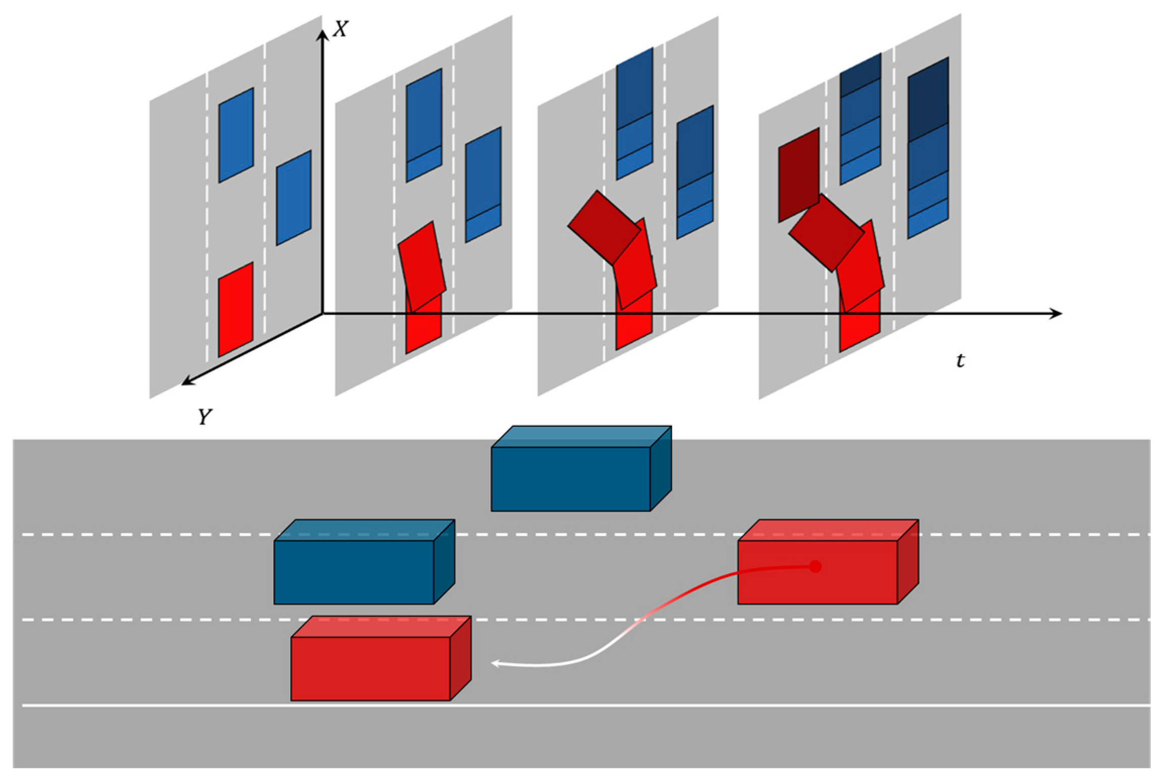
2.6. Development of a Lane-Changing and Obstacle-Avoidance Planning Scheme for Autonomous Vehicles Operating on Urban Roads

Vehicles in urban traffic environments may face static or dynamic obstacles during their journeys. Two methods for avoiding them include brake pedal application to decrease speed before the collision and steering wheel adjustment to avoid the collision. Using speed reduction may cause Energy waste and road congestion. Therefore, lane-changing is preferred when facing obstacles if the traffic conditions permit doing so. This paper aims to establish a lane-changing and obstacle-avoidance motion planning task under conditions permitting lane-changing maneuvers according to traffic regulations.

To establish a Cartesian coordinate system on a plane, the x-axis is set along the right side of the road, where the direction of travel in the lane is considered positive. As shown in the following Figure 8.

Establish collision avoidance constraints for autonomous vehicles on urban roads:

$$\begin{array}{c}RA\le P\le LA,P\in \{A_y(t),B_y(t),C_y(t),D_y(t)\},t\in [t_0,t_f]\\ \left\{\begin{array}{l}v(t)\ge 0\\ -\frac{\pi }{2}\le \theta (t)\le \frac{\pi }{2}\end{array}\right.\end{array}$$

(19)

In the motion process, the initial state $(x(t_0),y(t_0))$ must adhere to the requirements specified in the task. The state and control variables are given below:

$$[a(t_0),w(t_0),v(t_0),\Phi (t_0),\theta (t_0),x(t_0),y(t_0)]=[0,0,v_g,0,0,x_0,y_0]$$

(20)

At the termination time, $t_f$, the vehicle must be driving in the lane it has changed to. Given the assumption of a lane width of $H$, the state and control variables at that time are as follows:

$$[a(t_f),w(t_f),v(t_f),\Phi (t_f),\theta (t_f),y(t_f)]=[0,0,v_g,0,y_0\pm H]$$

(21)

Select Bolza performance index function:

$$\min J={\lambda }_1\cdot (t_f-t_0)+{\lambda }_2\cdot {\displaystyle \underset{t_0}{\overset{t_f}{\int }}{(w_i(t))}^{2}dt}$$

(22)

The Bolza performance index function considers the vehicle’s smoothness throughout its entire range and its primary objective of achieving the quickest lane change time.

The constraints of the vehicle’s kinematic model (5), ego vehicle constraint (7), the vertex coordinate constraint (12), two-vehicle collision avoidance constraint (13), road constraint (19), initial path constraint (20) and termination path constraint (21).

Thus, the above formulas comprise the optimal control problem, which allows simplification of this series of performance functions and other constraints:

$$\begin{array}{c}\min imizeJ={\lambda }_1\Phi [z(t_0),z(t_f),t_0,t_f]+{\lambda }_2\cdot {\displaystyle \underset{t_0}{\overset{t_f}{\int }}P[z(t),u(t),t]dt}\\ s.t\frac{dz(t)}{dt}=f[z(t),u(t),t]\\ D(z(t),u(t),t)=0\\ ND(z(t),u(t),t)\le 0\end{array}$$

(23)

Minimizing time weight is given by ${\lambda }_1$, while ${\lambda }_2$ is the smoothness weight for lane changes, with ${\lambda }_1+{\lambda }_2=1$. The state variable is $z(t)$, the control variable is $u(t)$, $t_0$ is the initial time, and $t_f$ is the termination time. The dynamics constraint is represented by $f$, while $D$ and $ND$ represent various equality and inequality constraints, respectively. The goal is to identify the control variable $u(t)$ and termination time $t_f$ satisfying constraint conditions and minimizing $J$.

3. Vehicle Trajectory Planning for Obstacle Avoidance Using the Gauss Pseudo-Spectral Approach

This chapter proposes a pseudo-spectral-based vehicle lane change and obstacle avoidance trajectory planning method, transforming a multi-constraint optimal control problem. It proceeds by discretizing the continuous-time problem using interval transformation and Lagrange interpolating functions. The output is a set of corresponding trajectories.

3.1. Methods for Solving Optimal Control Problems

A standard solution to address the optimal control problem mentioned above is to utilize variational and maximum principle methods to derive optimal conditions. These optimal conditions are solved indirectly to obtain the solution to the optimal control problem. Another strategy involves applying shooting and collocation methods to transform differential equations into a nonlinear programming problem. Among these methods, the preferred approach is the direct method using collocation. Collocation discretizes the optimal control problem and turns it into a numerical NLP problem, providing optimal solutions. The advantage of collocation is its ability to discretize both state and control variables, unlike shooting, which only gets control variables discretized. Therefore, in this article, we have used the pseudo-spectral method in collocation to determine the trajectory plan. As shown in the following Figure 9.

3.2. Trajectory Planning for Vehicle Obstacle Avoidance Using Gaussian Pseudo-Spectral Method

This section will use the optimal control model for vehicle obstacle avoidance obtained earlier and apply the Gaussian pseudo-spectral method to discretize both state and control variables in solving the optimal control problem. Specifically, we will employ Legendre-Gauss (LG) collocation to approximate state and control variables and transform the problem into a nonlinear programming problem.

Figure 10 mainly shows the framework of the trajectory planning method based on the Gaussian pseudospectral method. After the decision end issues a decision command, it is based on vehicle status and control variables, vehicle kinematics model, minimize performance metrics, vehicle constraints and collision avoidance constraints, boundary constraints composition of optimal control problem based on vehicle status, go through interval mapping, discretization of state variables and control variables, discretization of differential dynamic equations, discretization of the optimal control problem using Gaussian pseudospectral point matching method. The obtained results are solved using nonlinear programming problems, and the trajectory curve, state parameters, and control parameters are obtained.

Interval transformation:

The above optimal control time interval is $[t_0,t_f]$. In the Gaussian pseudo-spectral method, K-order Legendre polynomials are selected as the discrete points with LG points distributed in $\tau \in [-1,1]$. Therefore, the time interval of the optimal control problem needs to be transformed as follows:

$$\tau =\frac{2t}{t_f-t_0}-\frac{t_f+t_0}{t_f-t_0}$$

(24)

The optimal control problem that has been transformed can be described as follows:

$$\begin{array}{c}\min imizeJ={\lambda }_1\Phi [z(-1),z(1),t_0,t_f]+\frac{t_f-t_0}{2}{\lambda }_2\cdot {\displaystyle \underset{-1}{\overset{1}{\int }}P[z(\tau ),u(\tau ),\tau ]d\tau }\\ s.t\frac{dz(t)}{dt}=\frac{t_0-t_f}{2}f[z(\tau ),u(\tau ),\tau ]\\ D(z(\tau ),u(\tau ),\tau )=0\\ ND(z(\tau ),u(\tau ),\tau )\ne 0\end{array}$$

(25)

Discretizing both state and control variables is a crucial step in optimization:

In the normalized $\tau \in [-1,1]$, the Nth-order Lagrange interpolation function approximates the state variables and control variables.

$$\begin{array}{l}z(\tau )\approx Z(\tau )={\displaystyle \sum _{n=0}^N{Z}_n{L}_n(\tau )}\\ u(\tau )\approx U(\tau )={\displaystyle \sum _{n=0}^N{U}_n{L}_n(\tau )}\end{array}$$

(26)

The order of interpolation is represented by $N$. $L_n(\tau )$ denotes the Lagrange interpolation polynomial. $Z_n$ and $U_n$ represent collocation points used for state and control variables. Discretizing these points allows the approximation of a continuous function throughout the time domain.

The Lagrange interpolation polynomial shown above can be expressed as:

$$L_n(\tau )={\displaystyle \prod _{\begin{array}{l}i=0\\ i\ne n\end{array}}^N\frac{\tau -{\tau }_i}{{\tau }_n-{\tau }_i}}$$

(27)

Since the Lagrange-Gauss collocation does not include the state at the terminal time, the final state estimate can be expressed as:

$$z({\tau }_f)=z({\tau }_0)+{\displaystyle \underset{-1}{\overset{1}{\int }}P[z(\tau ),u(\tau ),\tau ]}d\tau$$

(28)

The discrete form of the equation is expressed using Gauss quadrature formula:

$$z({\tau }_f)-z({\tau }_0)-\frac{t_f-t_0}{2}{\displaystyle \sum _{n=0}^N{G}_{n}P[z({\tau }_n),u({\tau }_n),\tau ;t_0,t_f]}=0$$

(29)

where $G_n$ is the Gauss weight and ${\tau }_n$ is the LG point.

The integral term in the performance index is approximated by Gauss quadrature:

$$\min imizeJ={\lambda }_1\Phi [z(-1),z(1),t_0,t_f]+{\lambda }_2\cdot \frac{t_f-t_0}{2}{\displaystyle \sum _{n=0}^N{G}_{n}P[z({\tau }_n),u({\tau }_n),\tau ;t_0,t_f]}$$

(30)

3.3. The Discretization of Differential Dynamic Equations

Differential form exists in $\frac{dz(t)}{d\tau }=\frac{t_0-t_f}{2}f[z(\tau ),u(\tau ),\tau ]$, differentiate the Lagrange function to obtain $\frac{dz(\tau )}{d\tau }={\displaystyle \sum _{n=0}^N{Z}_n\stackrel{•}{L_n(\tau )}}$. Therefore, the dynamic differential equation constraint on the LG collocation point configuration is an algebraic constraint:

$${\displaystyle \sum _{n=0}^N{Z}_n\stackrel{•}{L_n(\tau )}}-\frac{t_f-t_0}{2}f[z({\tau }_n),u({\tau }_n),\tau ;t_0,t_f]=0$$

(31)

where $\stackrel{•}{L_n(\tau )}$ is the derivative of the Lagrange interpolation basis function.

Discretized form of optimal control problem:

Thus, the above optimal control problem is transformed into a nonlinear programming problem, and the expression of the nonlinear programming problem is:

$$\begin{array}{c}\min imizeJ={\lambda }_1(t_f-t_0)+{\lambda }_2\cdot \frac{t_f-t_0}{2}{\displaystyle \sum _{n=0}^N{G}_n[W_n{(\tau )}^2]}\\ s.t{\displaystyle \sum _{n=0}^N{Z}_n\stackrel{•}{L_n(\tau )}}-\frac{t_f-t_0}{2}f[z({\tau }_n),u({\tau }_n),\tau ;t_0,t_f]=0\\ z({\tau }_f)-z({\tau }_0)-\frac{t_f-t_0}{2}{\displaystyle \sum _{n=0}^N{G}_{n}P[z({\tau }_n),u({\tau }_n),\tau ;t_0,t_f]}=0\\ D(z(\tau ),u(\tau ),\tau ;t_0,t_f)=0\\ ND(z(\tau ),u(\tau ),\tau ;t_0,t_f)\ne 0\end{array}$$

(32)

Solving nonlinear programming problems.

This study applies the SQP sequential quadratic programming algorithm to solve nonlinear programming problems. The original problem is transformed into NLP using the direct method, and the MATLAB solver SNOPT, which is based on the SQP algorithm, is used, further promoting the application of the SQP algorithm. The SQP algorithm retains a crucial role in solving trajectory optimization problems. Most trajectory optimization problems that undergo discrete transformation into NLP through direct methods employ the SQP algorithm as the solution. Ultimately, solving the problem can ultimately yield the optimal trajectory for an urban road scene.

4. Simulation Results and Analysis

The chapter presents the design and simulation experiments of obstacle avoidance tasks for autonomous vehicles on urban roads. The proposed road scenario consists of three lanes, where every single lane of a bidirectional six-lane road is 3.75 meters wide. The center line coordinates of the road are $y_1=1.875$, $y_2=5.625$ and $y_3=9.375$. The simulation experiment parameters are presented in

Table 1. Simulation experiment parameters.

Parameter	Meaning	Value
$L_f$	Front overhang distance	$930 \mathrm{mm}$
$L$	Wheelbase	$2870 \mathrm{mm}$
$L_r$	Rear overhang distance	$910 \mathrm{mm}$
$L_b$	Vehicle width	$1800 \mathrm{mm}$
$RA$	Left roadside edge line	$0 \mathrm{m}$
$LA$	Right roadside edge line	$11.25 \mathrm{m}$
$d_{\min ,Lo}$	Minimum longitudinal safe distance	$0.67 \mathrm{m}\le d_{\min ,La}\le 2.17 \mathrm{m}$
$d_{\min ,La}$	Minimum lateral safe distance	$0.73 \mathrm{m}$
$\lambda$	Turning angle, time weight	$0<\lambda <1$
$v_{\max }$	maximum Speed limit	$50 \mathrm{km}/\mathrm{h}$
$a_{\max }$	Maximum acceleration	$0.48 {\mathrm{m}/\mathrm{s}}^2$
${\Phi }_{\max }$	Maximum turning angle	$32°$
$w_{\max }$	Front wheel’s steering angular velocity	$0.32 \mathrm{rad}/\mathrm{s}$

.

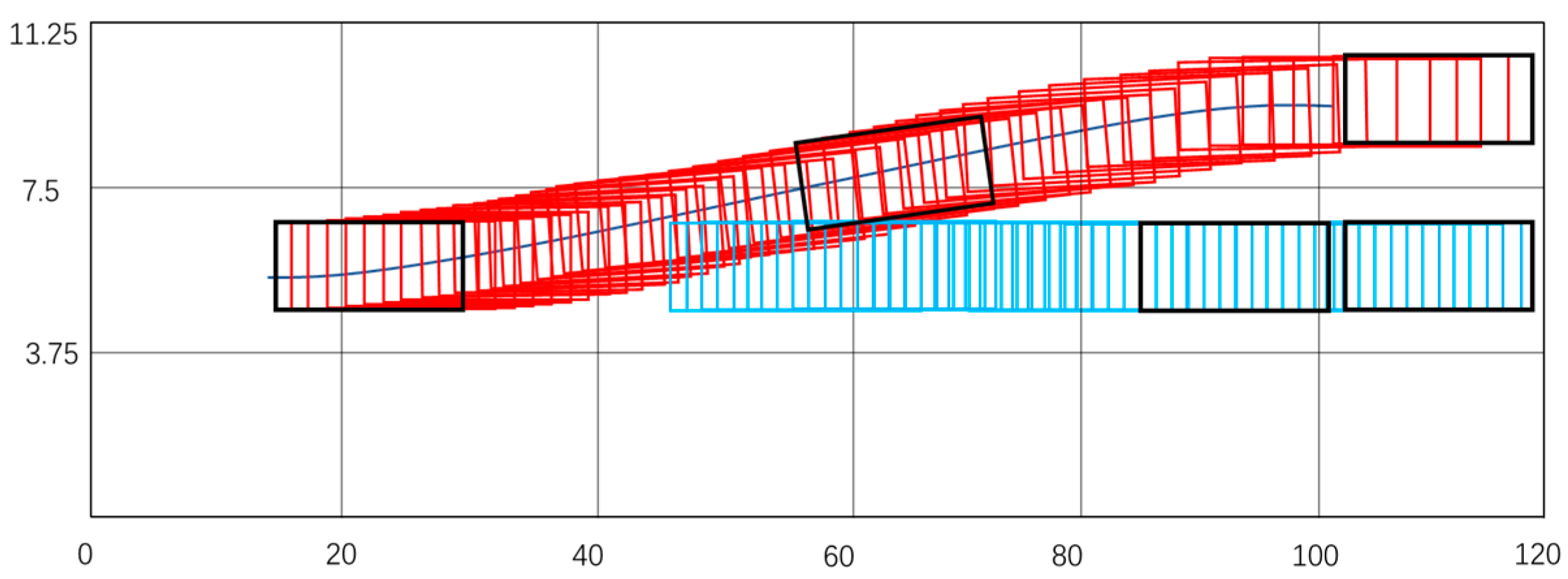
In the context of changing lanes and overtaking in a three-lane scenario, the road’s speed limit is $50 \mathrm{km}/\mathrm{h}$. Vehicle $A$ starts with an initial position of $(7.352,5.625)$ and an initial speed of $11 \mathrm{m}/\mathrm{s}$. There is an obstacle vehicle $B$ ahead at an initial position of $(17.352,5.625)$, driving at a uniform speed of $8 \mathrm{m}/\mathrm{s}$ along the current lane. After the decision-making stage, the optimal curve is planned based on the comfort weight and minimum time weight. During the simulation, the vehicle’s contour line includes the minimum longitudinal and lateral distance in two cases: (1) corner weight ${\lambda }_2=0.1$ and minimum time weight ${\lambda }_1=0.9$; (2) corner weight ${\lambda }_2=0.9$ and minimum time weight ${\lambda }_1=0.1$. Only these two cases are presented in this experiment, and the corresponding indicators can be calculated based on decision-making within this range.

Test 1 emphasizes minimizing avoidance and changing lanes time under a weight of corner ${\lambda }_2=0.1$ and minimum time ${\lambda }_1=0.9$. However, this weight results in a larger corner angle.

Test 2 emphasizes improving the occupants’ comfort by making the corner as smooth as possible under a weight of corner ${\lambda }_2=0.9$ and minimum time ${\lambda }_1=0.1$. However, this results in a longer avoidance time.

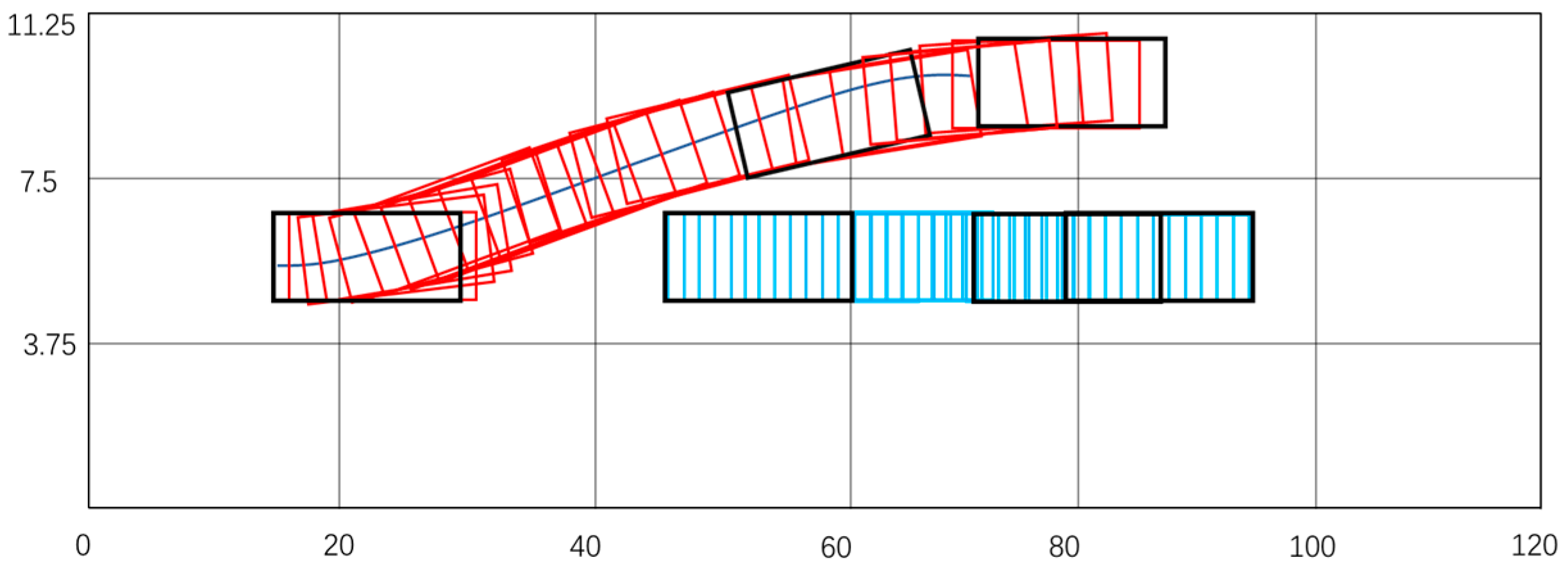
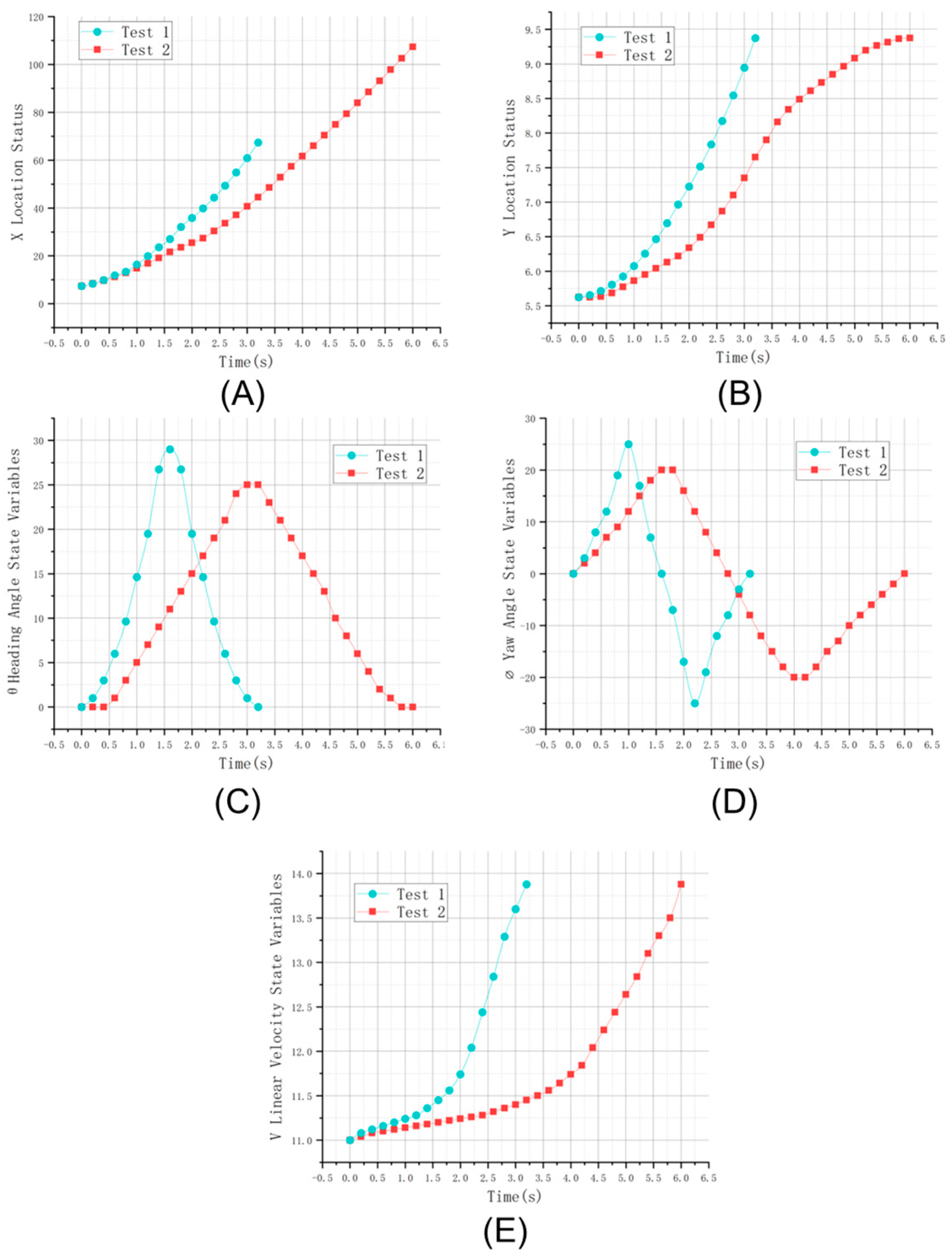
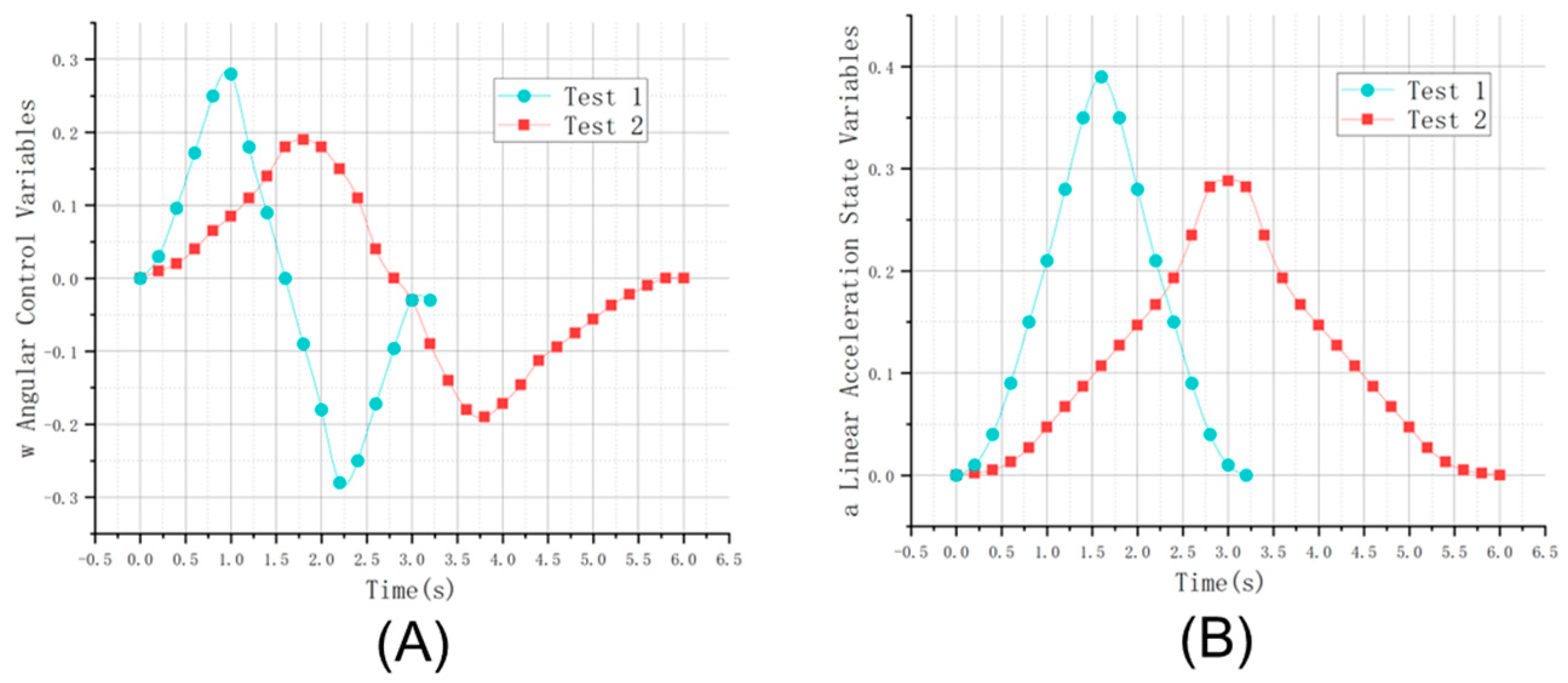
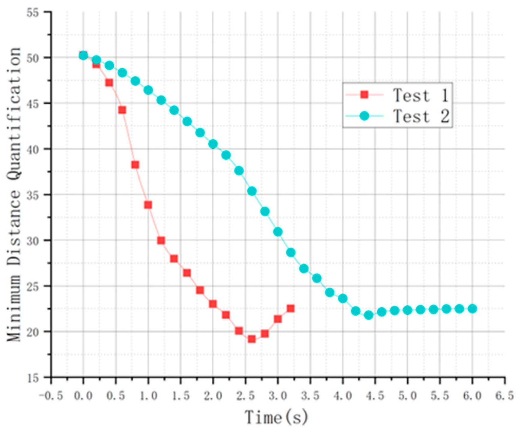
Figure 11 and Figure 12 presents the trajectory maps of test 1 and test 2, demonstrating safe obstacle avoidance in the depicted scenario. Figure 13 compares the state variables between the two tests, while Figure 14 compares the control variables. Figure 15 shows the comparison of minimum distance quantification, comparing the computational efficiency of the Gaussian Pseudo-spectral Method (GPM), Legendre Pseudo-spectral Method (LPM), and Direct Shooting Sparse Sequential Method (DSSSM) in the experiment.

After analyzing the simulation results, it is evident that:

Test 1 involved the movement of Vehicle $A$ from the initial position of $(7.532,5.625)$ to the final position of $\left(67.352,9.375\right)$. Figure 2 displays the state variables and control variables of the optimal trajectory of the vehicle. The time taken by the vehicle to complete the journey is $t_f=3.2 \mathrm{s}$. The vehicle starts accelerating from $11 \mathrm{m}/\mathrm{s}$ and reaches the maximum speed of $13.88 \mathrm{m}/\mathrm{s}$. The speed of the vehicle undergoes significant changes throughout the movement, with prominent peaks and valleys observed in state and control variables due to a focus on the minimum lane change time. The peak value of the longitudinal acceleration ‘a’, is $0.39 {\mathrm{m}/\mathrm{s}}^2$, and the angular velocity peaks at $0.28 \mathrm{rad}/\mathrm{s}$ and $-0.3 \mathrm{rad}/\mathrm{s}$. The highest heading and roll angles were measured with respect to the vehicle’s initial position, with the maximum heading angle ‘theta’ of $29$° and the roll angle of $25$° and $-26$° noticed in the study. The total number of interpolation points in this test was $31$, requiring a time of $0.846 \mathrm{s}$. Both state and control variables remain within their constraint conditions. Nevertheless, the high degree of lateral velocity change in this extreme scene may trigger passenger discomfort. However, the short lane change time could prevent injuries to passengers in critical situations while on the road.

Test 2 captured the movement of Vehicle A from the initial position of $(7.532,5.625)$ to the final position of $\left(107.352,9.375\right)$. The time taken by the vehicle to complete the movement is $t_f=6.0135 \mathrm{s}$. The vehicle’s speed shifts smoothly throughout the entire motion owing to the control variable constraints, which prevent sudden changes in line acceleration and angular velocity, leading to abrupt acceleration or deceleration. The peak value of the longitudinal acceleration ‘a’ is $0.288 {\mathrm{m}/\mathrm{s}}^2$, and the peak values of the angular velocity ‘w’ are $0.19 \mathrm{rad}/\mathrm{s}$ and $-0.20 \mathrm{rad}/\mathrm{s}$. In this scenario, the maximum heading angle ‘theta’ and roll angle are $25$°, $20$°, and $-19$°, respectively. This test had $17$ interpolation points that took $0.392 \mathrm{s}$ of time. Both state and control variables meet the constraints during the movement. A gradual acceleration policy was implemented during the vehicle’s acceleration stage instead of using the maximum peak value. Similar changes can be noticed in the tire roll angle information. The tire roll angle and angular velocity constraints account for this change, which enhances the vehicle’s longitudinal and lateral stability, thereby increasing the driver and passenger’s comfort level.

Figure 4 displays the operational data regarding the avoidance constraint model outlined in Section 2.4.2. It is capable of calculating the vehicle’s area within the bounding box, which was found to be $18.3675 {\mathrm{m}}^2$. The minimum vertex and contour area at the start are $50.24 {\mathrm{m}}^2$, and at the end, it was $22.5 {\mathrm{m}}^2$.

From the figure, it can be observed that the minimum contour area in the test 1 scenario is $19.981 {\mathrm{m}}^2$, and the minimum contour area in the test 2 scenario is $21.8 {\mathrm{m}}^2$, both of which are greater than the vehicle’s own frame area. Therefore, there is no collision between car $A$ and car $B$ in both scenarios. However, in the test 1 scenario, the minimum contour area is close to the frame area, which is a relatively dangerous lane change measure. Nonetheless, the model has already incorporated the minimum horizontal and vertical distance margins, so theoretically, there is no danger. Both the observations of the experimental data state variables and control variables and the quantification of the minimum distance for the experiment satisfy the safety conditions.

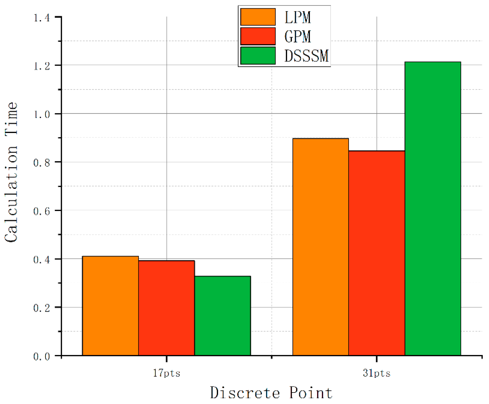
The computational efficiency of the Gaussian pseudo-spectral method (GPM), the Legendre pseudo-spectral method (LPM), and the direct shooting method (DSSSM) in the experiment is compared. The first two methods are based on Legendre polynomials for orthogonal configuration. All three methods are direct methods.

Legendre pseudo-spectral method (LPM): The position of the nodes is described by Legendre-Gauss-Lobatto (LGL) points in $t\in [-1,1]$, and −1 and 1 are included in the state approximation.

Direct shooting method (DSSSM): The direct shooting method discretizes the control variable in the time domain and transforms it into an NLP problem for solving. This method takes the control variable at the discrete time points as the design variable, and the state variable between the time nodes can be obtained by interpolation.

At the same time, the calculation times of LPM, GPM, and DSSSM are compared at 17 and 31 discrete points in the two scenarios mentioned above. As shown in the following Figure 16 and

Table 2. The calculation time of LPM, GPM, and DSSSM.

	LPM	GPM	DSSSM
17 pts	0.411	0.392	0.328
31 pts	0.897	0.812	1.224

.

The Figure 16 and Table 2 illustrate that DSSSM displays good computation speed when 17 discrete points are considered. However, as more discrete points are added, the algorithm’s performance declines and computation time increases. DSSSM can be applied to problems with arbitrary boundary conditions and is relatively easy to implement. Nonetheless, complex nonlinear problems incur slow convergence rates and numerous iterative calculations, leading to high computational costs. GPM, followed by LPM, exhibits superior computational speeds, particularly at 17 and 31 points, compared to DSSSM.

5. Conclusions

This paper presents an obstacle avoidance trajectory planning method for autonomous vehicles on urban roads using the Gauss pseudo-spectral method to describe the optimal control problem. The proposed method uses double-performance index functions, including time and steering angle optimization, to precisely model the vehicle’s constraints and avoidance constraints. The minimum safe distance model from the RSS is introduced to account for vehicle constraints. The Gauss pseudo-spectral method discretizes the problem into nonlinear programming problems, which are numerically solved. Two lane-changing scenarios are employed as experimental parameters in the simulation. Despite the adoption of extreme weights, all constraints are satisfied. In practical scenarios, the vehicle adjusts the weight based on the decision-making end to select the appropriate trajectory quickly, efficiently, and safely. Simulation outcomes manifest that GPM outperforms LPM in speed. Compared to the shooting method, GPM’s calculation speed is marginally faster at interpolation points of 17, whereas it is significantly slower at 31. Therefore, GPM exhibits better stability and speed among the methods proposed. However, GPM can only deal with simple lane-changing and avoidance scenarios, and continuous avoidance situations may result in high computational costs and delays in computation. In future work, these limitations can be overcome by implementing the finite element and pseudo-adaptive pseudo-spectral methods. The number of time intervals and polynomial orders can be dynamically adjusted based on each interval’s curvature and constraint equations to assign reasonable control points and intervals.