Adaptive MPC-Based Lateral Path-Tracking Control for Automatic Vehicles

Abstract

For continuously changing road conditions and vehicle operating states, the exactitude of vehicle path tracking has not been secured by model predictive control based on linear lateral stiffness. An amended square root cubature Kalman filter method based on the minimization of a new covariance of interest is proposed to calculate the tire lateral deflection force in real time. The ratio of the estimated tire force to the linear tire force was used as a ratio to adjust the lateral deflection stiffness, and an adaptive model predictive controller was built based on the vehicle path-tracking error model to correct the tire lateral deflection stiffness. Finally, an analysis based on the joint CarSim and Simulink simulation platform shows that compared to a conventional model predictive control (MPC) controller, a trajectory-following controller built based on this method can effectively reduce the lateral distance error and heading error of an autonomous vehicle. Especially under low adhesion conditions, the conventional MPC controllers will demonstrate large instability during trajectory tracking due to the deviation of the linear tire force calculation results, whereas the adaptive model predictive control (AMPC) controllers can correct the side deflection stiffness by estimating the tire force and still achieve stable and effective tracking of the target trajectory. This suggests that the proposed algorithm can improve the effectiveness of trajectory tracking control for autonomous vehicles, which is an important reference value for the optimization of autonomous vehicle control systems.

1. Introduction

In recent years, to alleviate traffic congestion and ensure driving safety, autonomous driving technology has become the most important developmental focus in the automotive industry [1]. Path tracking is an important part of autonomous driving. To improve the stability, comfort, and computational efficiency of path tracking, researchers have proposed various types of path-tracking algorithms, which mainly include proportional integral derivative (PID) [2], the linear-quadratic regulator (LQR) [3], the pure tracking algorithm [4] and the model predictive control (MPC) algorithm [5].

In most cases, the design of control algorithms for tracking depends on the system model of the controlled object, so the first step in the design of a control system is to create a vehicle dynamics model. In the literature, a classical two degrees of freedom vehicle dynamics model [6] has been developed to reduce the complexity of control strategy design and the resolution pressure of hardware algorithms and is widely used in the design of control algorithms. In addition, several experts and researchers have developed multi-degree-of-freedom vehicle dynamics models, including the three-degree-of-freedom model, which describes the steering behavior, and the seventeen-degree-of-freedom model, which fully describes the nonlinear characteristics of the tires, suspension, and kinematic constraints and more accurately describes the vehicle dynamics during the motion process. Many approaches to the development of control algorithms are based on theoretical mathematical models of vehicle dynamics, the calculation of physical quantities describing vehicle motion, such as angular velocity, and the subsequent development of a feedback control system for tracking. Liu et al. [7] pointed out that the steering performance of a two-degree-of-freedom linear model is similar to that of a fourteen-degree-of-freedom model under normal operating conditions, but there is a big difference under extreme operating conditions, and the tire profile, load transfer, and other vehicle characteristics, such as the kinematic constraints of the vehicle, need to be considered. Aouaouda et al. [8] proposed a nonlinear predictive control method to design a self-adaptive fuzzy controller using a two-domain linear vehicle model and an empirical tire model with a magic formula and iteratively adapted the membership function of the fuzzy controller and the control basis for vehicle control.

Traditional control methods struggle to effectively deal with multi-constrained problems. Compared with general feedback control and optimal control algorithms, MPC algorithms are especially good at solving multi-objective problems under optimal control systems [9]. With the development of online optimization and computer hardware, model predictive control has become an area of increasing interest in vehicle active safety [10,11] and path tracking [12]. Considering the problem of poor tracking of an automated vehicle when it slows down to change lanes in a given vicinity, Li et al. [13] proposed a lane change detection algorithm using two controllers and a steering tracking algorithm based on the combination of an MPC controller and a PI controller. Liang et al. [14] considered the problem that the saturation range of tire lateral deflection stiffness during cornering reduces the vehicle tracking performance on low-grip roads and proposed model predictive control (MPC). To address the problems with traditional tracking methods that may cause the car to crash and fall off the edge of the road, Gou et al. [15] proposed an implicit linear control method with model predictive control to design a tracking controller that can effectively deal with modeling errors by using different sampling times and prediction horizons. Wurts et al. [16] gave full consideration to the influence of surrounding vehicles on the self-driving vehicle and adopted a centralized control approach to ensure vehicle stability under extreme working conditions. Yakub et al. [17] proposed a MPC controller based on longitudinal velocity and considered the constraints of lateral oscillation dynamics in the vehicle model, which effectively reduced the trajectory tracking error and improved the stability of trajectory tracking. Ji et al. [18] proposed an integrated controller for real-time collision-free trajectory planning and tracking that builds an artificial 3D potential field based on road environment information and uses MPC with several constraints, including obstacle avoidance and stability constraints for basic control. Cui et al. [19] calculated trajectory safety bounds based on real-time pre-scan points to identify time-varying constraints in the forecast time domain and coordinated MPC control based on the relationship between trajectory tracking accuracy and stability. Active front-wheel steering with an additional steering angle can effectively improve the vehicle’s lateral stability on the highway, making active front-wheel steering a primary goal for optimizing trajectory control. Nathan et al. [20] addressed the complex and difficult-to-model pattern of nonlinear dynamics and environmental data uncertainty in the development of vehicle path-following controllers by using vehicle driving data to build a neural network model for predictive control (NNMPC), which is the proposed method. This method enables complex dynamic models to be predicted and the neural network models learned to be integrated into a non-linear solver, thereby increasing the reliability of MPC control.

Meanwhile, for automotive safety systems, oversteer and vehicle sideslip are easily produced when steering and driving, which can endanger personal safety in serious cases, so research on vehicle lateral stability is needed. The real-time and accurate estimation of the vehicle lateral motion state is the basis for the study of vehicle lateral stability control systems. Karn et al. [21] proposed a real-time algorithm for estimating the lateral deflection angle using low-cost sensors for vehicle lateral stability control, which combines model estimation and kinematics theory to compensate for the existence of road slope angle and variation in tire performance. Xiaoyu et al. [22] proposed a dynamic modeling and observation method to estimate the lateral force and lateral deflection angle and developed a trackless observer with a Kalman filter. Under different road conditions, the developed state observers are able to estimate the lateral deflection angle of the vehicle very well with very small estimation errors, which can provide reliable vehicle state information for vehicle stability management. Qi et al. [23] proposed a novel electronic stability control system for electric vehicles based on Kalman filtering for lateral deflection angle estimation, which achieves accurate lateral deflection angle estimation and improves the stability control system by using the combined model error and external disturbances as an extended Kalman filtering algorithm.

However, considering the complexity of tire structure and the influence of factors such as the road adhesion coefficient, there exists a complex nonlinear dynamic relationship between tire lateral force and slip angle. When the road environment and vehicle operating conditions constantly change, the tire lateral force obtained through linear lateral stiffness will have significant model errors, resulting in lower tracking accuracy in conventional MPC control for automatic vehicle path tracking [24]. Especially when the vehicle steering approaches the adhesion limit, MPC controllers designed based on linear lateral stiffness may pose traffic safety risks due to errors.

To this end, this paper uses a new minimization of covariance of an interest-based modified elementary amended square root cubature Kalman filter (ASRCKF) to estimate vehicle front and rear tire side forces based on a vehicle model. Next, an adaptive model predictive control (AMPC) algorithm based on the vehicle tracking error model is proposed by developing a tuning criterion for adaptive tire side bending stiffness using the ratio of the estimated tire side force to the estimated linear value of tire side bending stiffness as a scaling factor. Finally, the proposed AMPC controller is validated by building a joint simulation based on the CarSim and Simulink platforms.

2. Path-Tracking Error Modeling of Vehicles

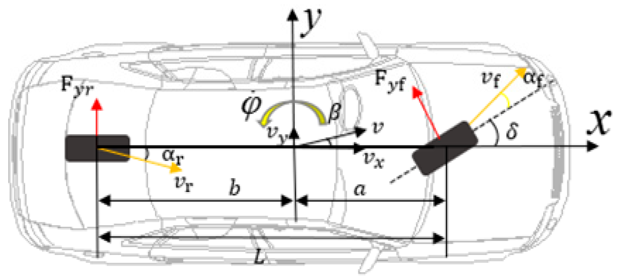
2.1. Vehicle Dynamics Model

The task of path tracking is to rapidly and stably track a reference path. In this study, we controlled the steering of the front wheels to accomplish the lateral path-tracking task of the vehicle. A 2-DOF vehicle dynamics model was created assuming that the vehicle is moving at a constant speed and ignoring the effects of the suspension system, transverse and longitudinal tire coupling forces, and aerodynamics [25], as shown in Figure 1.

The equation of lateral motion is given by:

$$m({\dot{v}}_y+{\dot{v}}_x\dot{\phi })=F_{\mathrm{yf}}+F_{\mathrm{yr}}$$

(1)

The equation of motion of the transverse pendulum is given by:

$$I_{\mathrm{z}}\ddot{\phi }=a{F}_{\mathrm{yf}}-b{F}_{\mathrm{yr}}$$

(2)

where $m$ is the vehicle mass; $v_x$ and $v_y$ denote the longitudinal and transverse speeds of the vehicle in the body coordinate system; $F_{\mathrm{yf}}$ and $F_{\mathrm{yr}}$ are the lateral forces on the front and rear tires, respectively; $I_z$ is the torque of the vehicle about the axis; $\dot{\phi }$ is the angular velocity of the vehicle’s pendulum; and $a$ and $b$ denote the distances from the center of mass of the vehicle to the front and rear axles.

When the lateral deflection angle of the tire is small, the relationship between the lateral force and the lateral deflection angle is linear, and using the small angle assumption, the tire lateral force can be linearized as:

$$\begin{array}{l}{F}_{\mathrm{yf}}={\overline{C}}_{\alpha \mathrm{f}}{\alpha }_{\mathrm{f}}={\overline{C}}_{\alpha \mathrm{f}}(\delta -\frac{v_y+a\dot{\phi }}{v_x})\\ F_{\mathrm{yr}}={\overline{C}}_{\alpha \mathrm{r}}{\alpha }_{\mathrm{r}}={\overline{C}}_{\alpha \mathrm{r}}(-\frac{v_y-b\dot{\phi }}{v_x})\end{array}$$

(3)

where ${\overline{C}}_{\alpha \mathrm{f}}$ and ${\overline{C}}_{\alpha \mathrm{r}}$ denote the linear lateral deflection stiffnesses of the front and rear tires, respectively, and their values are two times the individual tire deflection stiffness; $\delta$ is the front wheel rotation angle; and ${\alpha }_{\mathrm{f}}$ and ${\alpha }_{\mathrm{r}}$ are the front and rear tire deflection angles, respectively.

Substituting Equation (3) into Equations (1) and (2), the vehicle dynamics model can be obtained:

$$\left\{\begin{array}{c}{\dot{v}}_y=\frac{{\overline{C}}_{\alpha \mathrm{f}}+{\overline{C}}_{\alpha \mathrm{r}}}{m{v}_x}{v}_y+(\frac{a{\overline{C}}_{\alpha \mathrm{f}}-b{\overline{C}}_{\alpha \mathrm{r}}}{m{v}_x}-v_x)\dot{\phi }-\frac{{\overline{C}}_{\alpha \mathrm{f}}}{m}\delta \hfill \\ \ddot{\phi }=\frac{a{\overline{C}}_{\alpha \mathrm{f}}-b{\overline{C}}_{\alpha \mathrm{r}}}{I_z{v}_x}{v}_y+\frac{a^2{\overline{C}}_{\alpha \mathrm{f}}+b^2{\overline{C}}_{\alpha \mathrm{r}}}{I_z{v}_x}\dot{\phi }-\frac{a{\overline{C}}_{\alpha \mathrm{f}}}{I_z}\delta \hfill \end{array}\right.$$

(4)

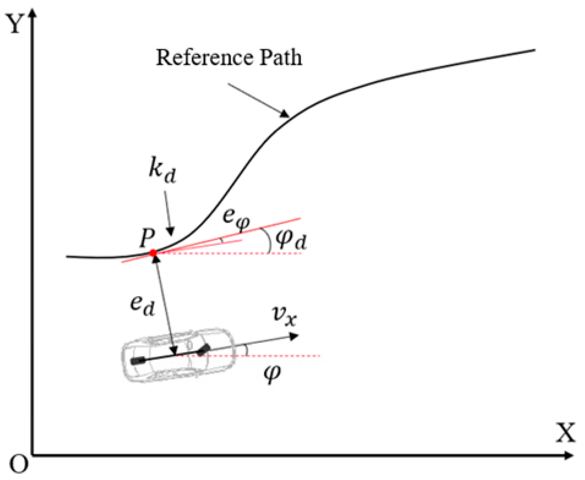
2.2. Tracking Model That Considers Trajectory Curvature

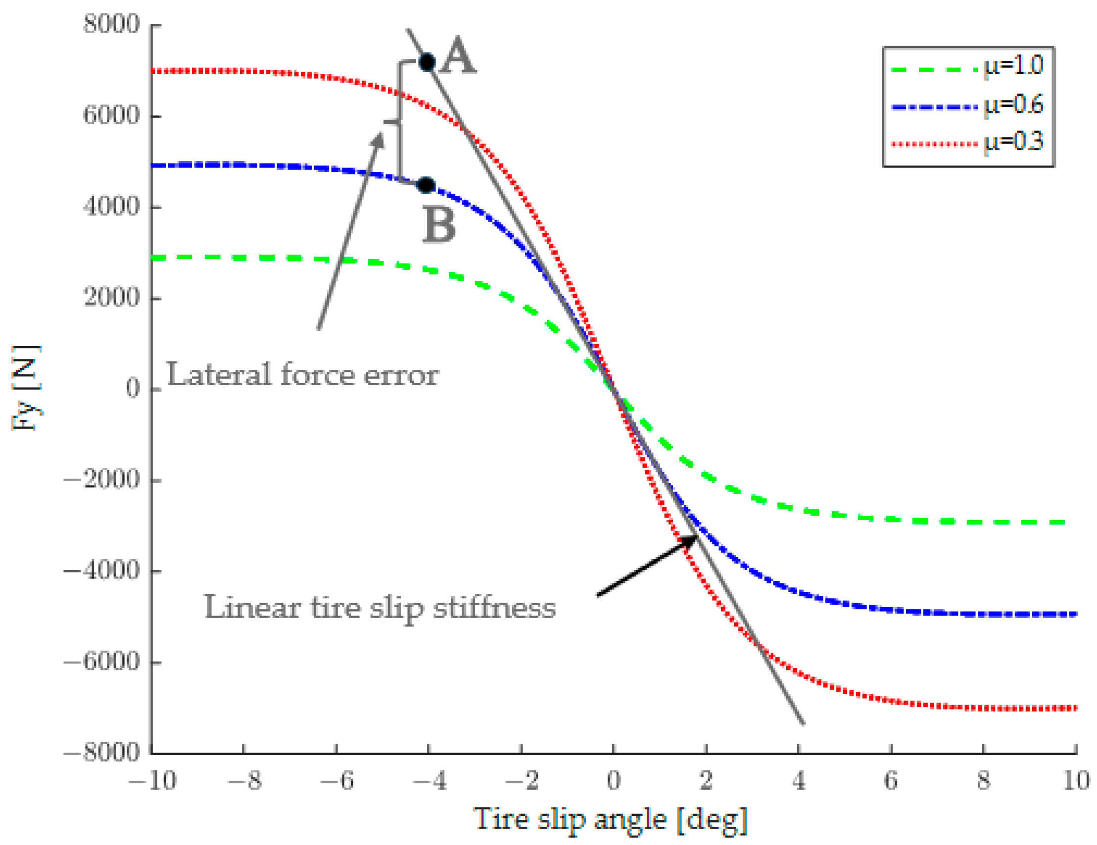
When a vehicle is traveling along a trajectory, the trajectory curvature plays an important role in steering characteristics and driving stability. Since this will directly affect the trajectory tracking accuracy of the vehicle, a tracking error model that considers the trajectory curvature should be established [26]. As shown in Figure 2, assuming that the reference path in the figure is obtained by smoothing the path obtained from the planning module using a B-spline curve, $P$ is the projection point of the center of mass of the vehicle on the reference trajectory, $e_d$ is the distance between the center of mass of the vehicle and the projection point, $\phi$ is the actual heading angle of the vehicle, ${\phi }_d$ is the angle between the tangent direction of the reference path and the X-axis of the ground coordinate system, and $e_{\phi }$ is the steering deviation of the vehicle.

According to the positional relationship of the vehicle and the reference path, the tracking error equation that considers the trajectory curvature can be expressed as:

$$\left\{\begin{array}{l}{\dot{e}}_{\phi }=\dot{\phi }-k_d\dot{s}\\ {\dot{e}}_d=v_x\sin (e_{\phi })+v_y\cos (e_{\phi })\end{array}\right.$$

(5)

where $k_{\mathrm{d}}$ is the curvature at the point $P$, and $\dot{s}$ is the rate at which the projected point $P$ moves along the reference path.

$$\dot{s}=\frac{1}{1-k_d{e}_d}\left[v_x\cos (e_{\phi })-v_y\sin (e_{\phi })\right]$$

(6)

when the vehicle is at a small angle front wheel turn, and as such, the above equation can be simplified as:

$$\left\{\begin{array}{l}{\dot{e}}_{\phi }=\dot{\phi }-\frac{k_d{v}_x}{1-k_d{e}_d}=\dot{\phi }-k_d{v}_x\\ {\dot{e}}_d=v_x{e}_{\phi }+v_y\end{array}\right.$$

(7)

Combining Equation (4) and Equation (7), let $x={[\begin{array}{cccc}{v}_x& \dot{\phi }& e_d& e_{\phi }\end{array}]}^T$ be the state quantity, $u=\delta$ be the control input quantity, $v={[\begin{array}{cccc}0& 0& 0& -k_d{v}_x\end{array}]}^T$ be the disturbance input quantity, and $y={[\begin{array}{ccc}\dot{\phi }& e_d& e_{\phi }\end{array}]}^T$ be the output quantity of the system. In this case, the vehicle tracking error model is:

$$\left\{\begin{array}{l}\dot{x}=Ax+Bu+v\\ y=Cx\end{array}\right.$$

(8)

$$\begin{gathered} A=\left[\begin{array}{cccc}\frac{{\overline{C}}_{\alpha \mathrm{f}}+{\overline{C}}_{\alpha \mathrm{r}}}{m{v}_x}& \frac{a{\overline{C}}_{\alpha \mathrm{f}}-b{\overline{C}}_{\alpha \mathrm{r}}}{m{v}_x}-v_x& 0& 0\\ \frac{a{\overline{C}}_{\alpha \mathrm{f}}-b{\overline{C}}_{\alpha \mathrm{r}}}{I_z{v}_x}& \frac{a^2{\overline{C}}_{\alpha \mathrm{f}}+b^2{\overline{C}}_{\alpha \mathrm{r}}}{I_z{v}_x}& 0& 0\\ 1& 0& 0& v_x\\ 0& 1& 0& 0\end{array}\right] \\ B={\left[\begin{array}{cccc}-\frac{{\overline{C}}_{\alpha \mathrm{f}}}{m}& -\frac{a{\overline{C}}_{\alpha \mathrm{f}}}{I_z}& 0& 0\end{array}\right]}^T \\ C=\left[\begin{array}{c}\begin{array}{cccc}0& 1& 0& 0\end{array}\\ \begin{array}{cccc}0& 0& 1& 0\end{array}\\ \begin{array}{cccc}0& 0& 0& 1\end{array}\end{array}\right] \end{gathered}$$

2.3. Tire Model

The above is due to the complex structure of the tire and the nonlinearity of its dynamic behavior. In this paper, the magic formula proposed by Pacejka et al. [27] is used. Figure 3 shows the lateral force and slip angle curves of the tire under different pavement adhesion coefficients determined by the magic formula when the vertical load is 7000 N. It can be seen that the linear tire lateral force based on linear tire slip stiffness obtained at point A is significantly larger than the nonlinear tire lateral force obtained at point B under the same tire slip angle condition. Therefore, it is necessary to develop an MPC controller to adjust the tire slip stiffness in real time according to the tire lateral force, because the lateral force determined based on the linear tire slip stiffness cannot respond to the change in the actual lateral force.

3. ASRCKF-Based Lateral Force Estimator

3.1. Vehicle System Modeling with ASRCKF Algorithm

The discrete equation of state and observation equation of the system are expressed as [28]:

$$\left\{\begin{array}{l}{x}_{\tau +1}=f\left(x_{\tau }\right)+w_{\tau }\\ z_{\tau +1}=h\left(x_{\tau +1}\right)+v_{\tau +1}\end{array}\right.$$

(9)

where $w_{\tau }$ is the process noise and $v_{\tau +1}$ is the measurement noise.

When defining the vehicle’s yaw rate as $\dot{\phi }$, lateral forces on the front and rear axles are $F_{\mathrm{yf}}$ and $F_{\mathrm{yr}}$, their first-order derivatives ${\dot{F}}_{\mathrm{yf}}$ and ${\dot{F}}_{\mathrm{yr}}$ constitute the state variable $x={[\begin{array}{ccccc}\dot{\phi }& F_{\mathrm{yf}}& {\dot{F}}_{\mathrm{yf}}& F_{\mathrm{yr}}& {\dot{F}}_{\mathrm{yr}}\end{array}]}^T$, the transverse angular rate and lateral acceleration constitute the observation $z={[\begin{array}{cc}\dot{\phi }& a_y\end{array}]}^T$, and the input $u$ is the front wheel angle $\delta$. The nonlinear equation of state and observation function of the vehicle system can thus be obtained:

$$f(x_{\tau })=\left[\begin{array}{ccccc}1& \frac{a\cos \delta T}{I_z}& 0& -\frac{bT}{I_z}& 0\\ 0& 1& T& 0& 0\\ 0& 0& 1& 0& 0\\ 0& 0& 0& 1& T\\ 0& 0& 0& 0& 1\end{array}\right]x_{\tau }$$

(10)

$$\left\{\begin{array}{l}{h}_1(x_{\tau +1})=x_{1,\tau }\\ h_2(x_{\tau +1})=\frac{F_{\mathrm{yf}}+F_{\mathrm{yr}}}{m}-v_x\dot{\phi }\end{array}\right.$$

(11)

Combining Equations (9)–(11), the tire lateral force estimator is designed by the ASRCKF algorithm:

(1)

Initialization

The initial values of the state ${\widehat{x}}_{\tau |\tau }$ and the covariance matrix $P_{\tau |\tau }$ are determined

$$\begin{array}{l}{\widehat{x}}_{\tau }=E(x_0)\\ P_{\tau }=E\left[\left(x_0-{\widehat{x}}_{\tau }\right){\left(x_0-{\widehat{x}}_{\tau }\right)}^T\right]\end{array}$$

(12)

(2)

Time Updates

The initial values of ${\widehat{x}}_{\tau |\tau }$ and $P_{\tau |\tau }$ at time $\tau$ yield the volume point $x_{\tau |\tau }^i$:

$$\begin{array}{l}{P}_{\tau |\tau }={S_{\tau }{S}_{\tau }}^T\\ x_{\tau |\tau }^i=S_{\tau }{\xi }_i+{\widehat{x}}_{\tau |\tau },i=1,2,\dots ,2n\end{array}$$

(13)

where $S_{\tau }$ is the square root of the covariance $P_{\tau |\tau }$, ${\xi }_i$ is the basic volume points, $I_m$ is the unit matrix, and $m$ is the dimension of the state vector.

$${\xi }_i=\left\{\begin{array}{cc}\sqrt{m}{I}_m,& i=1,2,\dots ,m\\ -\sqrt{m}{I}_m,& i=m+1,m+2,\dots ,2m\end{array}\right.$$

(14)

The volume point after passing through the state transfer equation can be given as:

$$x_{\tau |\tau }^{i\ast }=f\left(x_{\tau |\tau }^i\right)$$

(15)

Using the transferred volume points, one can derive the predicted value of the state $x_{\tau +1|\tau }^i$ and the square root of the predicted covariance $S_{\tau +1|\tau }$ as such:

$$\begin{array}{l}{\widehat{x}}_{\tau +1|\tau }=\frac{1}{2n}{\displaystyle \sum _{i=1}^{2n}{x}_{\tau +1|\tau }^{i\ast }}\\ S_{\tau +1|\tau }=Tria\left(\left[{\chi }_{\tau +1|\tau }^{i\ast },\sqrt{Q_{\tau }}\right]\right)\end{array}$$

(16)

where $Tria$ denotes the $QR$ matrix operation, and ${\chi }_{\tau +1|\tau }^{i\ast }$ is the central weighting matrix.

$${\chi }_{\tau +1|\tau }^{i\ast }=\frac{1}{\sqrt{2n}}(x_{\tau +1|\tau }^{1\ast }-{\widehat{x}}_{\tau +1|\tau },x_{\tau +1|\tau }^{2\ast }-{\widehat{x}}_{\tau +1|\tau },\dots ,x_{\tau +1|\tau }^{2n\ast }-{\widehat{x}}_{\tau +1|\tau })$$

(17)

(3)

Measurement Updates

The volume point can be determined as follows:

$$x_{\tau +1|\tau }^i=S_{\tau +1|\tau }{\xi }_i+{\widehat{x}}_{\tau +1|\tau }$$

(18)

After the volume point is passed through the observation function, the following is true:

$$z_{\tau +1|\tau }^i=h\left(x_{\tau +1|\tau }^i\right)$$

(19)

The observed predictions ${\widehat{z}}_{\tau +1|\tau }$, the square root of the new interest error covariance matrix $S_{zz,\tau +1|\tau }$, and the new interest $r_{\tau +1}$ are derived using the transferred volumetric points to further compute the observed covariance matrix $p_{zz,\tau +1|\tau }$ and the reciprocal covariance matrix $p_{xz,\tau +1|\tau }$.

$$\begin{array}{l}{\widehat{z}}_{\tau +1|\tau }=\frac{1}{2n}{\displaystyle \sum _{i=1}^{2n}{z}_{\tau +1|\tau }^i}\\ S_{zz,\tau +1|\tau }=Tria\left[\left(Z_{\tau +1|\tau },\sqrt{R_{\tau +1}}\right)\right]\\ r_{\tau +1}=z_{\tau +1}-{\widehat{z}}_{\tau +1|\tau }\\ P_{zz,\tau +1|\tau }=S_{zz,\tau +1|\tau }{S}_{zz,\tau +1|\tau }^T\\ P_{xz,\tau +1|\tau }={\chi }_{\tau +1|\tau }{Z}_{\tau +1|\tau }^T\end{array}$$

(20)

where $Z_{\tau +1|\tau }$ and ${\chi }_{\tau +1|\tau }$ are the weighting matrices.

$$Z_{\tau +1|\tau }=\frac{1}{\sqrt{2n}}[z_{\tau +1|\tau }^1-{\widehat{z}}_{\tau +1|\tau },z_{\tau +1|\tau }^2-{\widehat{z}}_{\tau +1|\tau },\dots ,z_{\tau +1|\tau }^{2n}-{\widehat{z}}_{\tau +1|\tau }]$$

(21)

$$Z_{\tau +1|\tau }=\frac{1}{\sqrt{2n}}[z_{\tau +1|\tau }^1-{\widehat{z}}_{\tau +1|\tau },z_{\tau +1|\tau }^2-{\widehat{z}}_{\tau +1|\tau },\dots ,z_{\tau +1|\tau }^{2n}-{\widehat{z}}_{\tau +1|\tau }]$$

(22)

(4)

Status Updates

The $\tau +1$ momentary filter gain $K_{\tau +1|\tau }$, the state estimate ${\widehat{x}}_{\tau +1|\tau +1}$, and the estimation error covariance $S_{\tau +1|\tau +1}$ can be determined as follows:

$$\begin{array}{l}{K}_{\tau +1|\tau }=p_{xz,\tau +1|\tau }{\left(p_{zz,\tau +1|\tau }\right)}^{-1}\\ {\widehat{x}}_{\tau +1|\tau +1}={\widehat{x}}_{\tau +1|\tau }+K_{\tau +1|\tau }\left(z_{\tau +1|\tau }-{\widehat{z}}_{\tau +1|\tau }\right)\\ S_{\tau +1|\tau +1}=Tria\left[\left({\chi }_{\tau +1|\tau }-K_{\tau +1|\tau }{Z}_{\tau +1|\tau },K_{\tau +1}\sqrt{R_{\tau +1}}\right)\right]\end{array}$$

(23)

(5)

Factor Correction

The coefficients are corrected based on the minimum new interest covariance [20], which is first corrected for the $\tau$ moment estimate ${\tilde{x}}_{\tau |\tau }$:

$${\tilde{x}}_{\tau |\tau }={\widehat{x}}_{\tau |\tau }+D_{\tau }{r}_{\tau +1}$$

(24)

where $D_{\tau }={\left[\begin{array}{cccc}{d}_1& d_2& \cdots & d_n\end{array}\right]}^T$ denotes the coefficients of the observation vector.

The corrected estimation error covariance as well as the prediction error skewness can thus be obtained:

$$\begin{array}{l}{\tilde{P}}_{\tau |\tau }=P_{\tau |\tau }+D_{\tau }{P}_{zz,\tau +1|\tau }{D}_{\tau }^T-P_{\tau |\tau }{M}_{\tau }^T{N}_{\tau +1}^T{D}_{\tau }^T-D_{\tau }{N}_{\tau +1}{M}_{\tau }{P}_{\tau |\tau }^T\\ {\tilde{P}}_{\tau +1|\tau }=P_{\tau +1|\tau }+E_{\tau }{P}_{zz,\tau +1|\tau }{E}_{\tau }^T-P_{\tau +1|\tau }{N}_{\tau +1}^T{E}_{\tau }^T-E_{\tau }{N}_{\tau +1}^T{P}_{\tau +1|\tau }\end{array}$$

(25)

where $M_{\tau }=\frac{\partial f}{\partial x_{\tau }}{|}_{x_{\tau }=x_{\tau +1|\tau }}$ and $N_{\tau +1}=\frac{\partial h}{\partial x_{\tau }}{|}_{x_{\tau }=x_{\tau +1|\tau }}$ are the state transfer matrix and the linearized approximation matrix $E_{\tau }=M_{\tau }{D}_{\tau }$ of the observation function, respectively.

This gives the corrected new interest covariance:

$${\tilde{P}}_{zz,\tau +1|\tau }=L_{\tau +1}{P}_{zz,\tau +1}{L}_{\tau +1}^T-{\mathsf{\Gamma }}_{\tau +1}{L}_{\tau +1}^T-L_{\tau +1}{\mathsf{\Gamma }}_{\tau +1}$$

(26)

In Equation (26), $L_{\tau +1}=N_{\tau +1}{P}_{\tau +1|\tau }{N}_{\tau +1}^T$, ${\mathsf{\Gamma }}_{\tau +1}=N_{\tau +1}{E}_{\tau }$.

The modified new interest covariance matrix can then be minimized as follows:

$$\frac{\partial {\tilde{P}}_{zz,\tau +1|\tau }}{\partial L_{\tau +1}}=\left(P_{zz,\tau +1|\tau }+P_{zz,\tau +1|\tau }^T\right)L_{\tau +1}-{\mathsf{\Gamma }}_{\tau +1}-{\mathsf{\Gamma }}_{\tau +1}^T=0$$

(27)

$$L_{\tau +1}=\left(P_{zz,\tau +1|\tau }+P_{zz,\tau +1|\tau }^T\right)\left({\mathsf{\Gamma }}_{\tau +1}+{\mathsf{\Gamma }}_{\tau +1}^T\right)$$

(28)

when $P_{zz,\tau +1|\tau }$ and $P_{\tau +1|\tau }$ are symmetric matrices, Equation (27) can be expressed as:

$$L_{\tau +1}=P_{zz,\tau +1|\tau }^{-1}{\mathsf{\Gamma }}_{\tau +1}$$

(29)

The factor adjustment that satisfies the minimum value for the updated covariance matrix can be translated as:

$$D_{\tau }={\left(N_{\tau +1}{M}_{\tau }\right)}^{+}{P}_{zz,\tau +1|\tau }^{-1}{\mathsf{\Gamma }}_{\tau +1}$$

(30)

where the matrix $N_{\tau +1}{M}_{\tau }$ may be a singular array, and ${\left( \right)}^{+}$ is the $Moore-Penrose$ of the matrix.

Finally, utilizing the updated state estimation values obtained through the aforementioned adjustments, together with the estimated error covariance, filtering is performed once again through Equations (13)–(23) in a recursive manner.

In

Table 1. List of symbols.

Symbol	Meaning	Unit
A	State-space system matrix
a, b	Front and rear semi-wheelbases	m
B	Control action matrix
${\overline{C}}_{\alpha \mathrm{f}}$	Linear lateral deflection stiffness of the front tire	N·rad−1
${\overline{C}}_{\alpha \mathrm{r}}$	Linear lateral deflection stiffness of the rear tire	N·rad−1
$D_{\tau }$	Coefficients of the observation vector
$e_d$	Lateral position error	m
$e_{\phi }$	Heading angle error	rad
$F_{\mathrm{yf}}$	Lateral force on the front tire	N
$F_{\mathrm{yr}}$	Lateral force on the rear tire	N
$I_m$	Unit matrix
$I_z$	Torque of the vehicle about the axis	kg·m2
J	Cost function
$k_{\mathrm{d}}$	Road curvature
$K_{\tau +1|\tau }$	Filter gain
m	Total vehicle mass	kg
$M_{\tau }$	State transfer matrix
$N_c$	Number of steps of the control horizon
$N_p$	Number of steps of the prediction horizon
$N_{\tau +1}$	Linearized approximation matrix
$P_{\tau |\tau }$	Covariance matrix
$P_{xz,\tau +1|\tau }$	Reciprocal covariance matrix
s	Distance covered along the path	m
$S_{\tau }$	Square root of the covariance
$S_{\tau +1|\tau }$	Square root of predicted covariance
$S_{zz,\tau +1|\tau }$	Square root of the new interest error covariance matrix
t	Time	s
T	Sampling time	s
u	Control action vector
$v_x$	Longitudinal vehicle speed	m·s−1
$v_y$	Lateral vehicle speed	m·s−1
$v_{\tau +1}$	Measurement noise
$w_{\tau }$	Process noise
x	State vector
${\widehat{x}}_{\tau |\tau }$	Initial value
$x_{\tau |\tau }^i$	Volume point
$x_{\tau +1|\tau }^i$	State prediction
${\tilde{x}}_{\tau |\tau }$	State estimate
X, Y	Coordinates in the global reference system	m
$Z_{\tau +1|\tau }$	Weighting matrix
${\tilde{x}}_{\tau |\tau }$	State estimate
X, Y	Coordinates in the global reference system	m
$Z_{\tau +1|\tau }$	Weighting matrix
δ	Front wheel steering angle	rad
β	Vehicle sideslip angle	rad
$\phi$	Yaw angle	rad
${\xi }_i$	Basic volume point
${\chi }_{\tau +1|\tau }^{i\ast }$	Central weighting matrix
${\chi }_{\tau +1|\tau }$	Weighting matrix

, all symbols used in this paper are listed and explained.

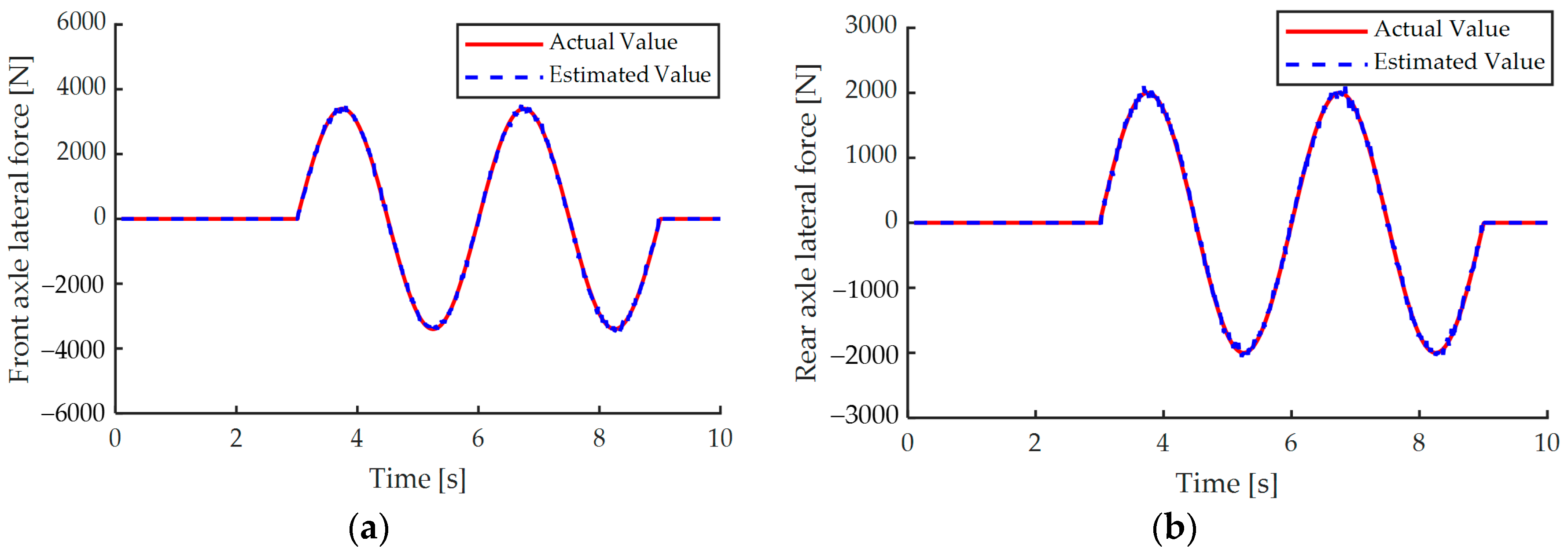
3.2. Validation of the Tire Lateral Force Estimator

To validate the effectiveness of the above lateral force estimator, a joint simulation was performed using the CarSim and Simulink platforms: the actual tire lateral forces from the CarSim vehicle model were compared with the estimates obtained from the ASRCKF estimator. The vehicle was set to drive at an initial speed of 60 kph on a road with an adhesion coefficient of 0.8, and the steering wheel input was a sinusoidal input signal with a period of 3 s and an amplitude of ${60}^{°}$. As shown in Figure 4, the results of estimating the lateral force of the vehicle’s tires show that, under sinusoidal signal input conditions, the designed ASRCKF estimator can effectively estimate changes in the lateral forces of the vehicle’s front and rear tires and provide accurate vehicle data for the design of the next controller.

4. Path-Tracking Controller Design

4.1. Guidelines for Adjusting Lateral Deflection Stiffness

The curves of the lateral force of the tire and the slip angle of the tire for different vertical loads given in Figure 3 show that there is a more accurate linear relationship only when the slip angle of the tire is small. In the presence of vertical load displacements and for large slip angles, the lateral force values calculated with linear slip stiffness show significant errors compared to the actual values [29]. To minimize the impact of linear slip stiffness on control efficiency, this study developed a criterion for setting the linear slip stiffness of a tire. However, if the tire slip stiffness values ${\widehat{F}}_{\mathrm{yf}}/{\alpha }_{\mathrm{f}}$ and ${\widehat{F}}_{\mathrm{yr}}/{\alpha }_{\mathrm{r}}$ are estimated directly to estimate the tire slip angle values ${\widehat{C}}_{\alpha \mathrm{f}}$ and ${\widehat{C}}_{\alpha \mathrm{r}}$, outlier estimation residuals may occur, and it is impossible to solve when ${\alpha }_{\mathrm{f}}=0$ or ${\alpha }_{\mathrm{r}}=0$ appears. Therefore, this paper uses the ratio of the estimated tire lateral force to the linear tire force to correct the slip stiffness. As a result, the proportion factor of tire slip stiffness is expressed as:

$${\chi }_{\mathrm{f}}={\widehat{F}}_{\mathrm{yf}}/F_{\mathrm{yf}}, {\chi }_{\mathrm{r}}={\widehat{F}}_{\mathrm{yr}}/F_{\mathrm{yr}}$$

(31)

Therefore, the corrected tire lateral deflection stiffness is expressed as:

$${\widehat{C}}_{\alpha \mathrm{f}}={\chi }_{\mathrm{f}}{\overline{C}}_{\alpha \mathrm{f}}, {\widehat{C}}_{\alpha \mathrm{r}}={\chi }_{\mathrm{r}}{\overline{C}}_{\alpha \mathrm{r}}$$

(32)

To prevent the scale factors ${\chi }_{\mathrm{f}}$ and ${\chi }_{\mathrm{r}}$ from being unsolvable when the calculated value of the linear tire force is 0, the scale factor is defined to take on a value of one when the tire side deflection angle ${\alpha }_{\mathrm{f}}$ or ${\alpha }_{\mathrm{r}}$ is less than ${0.1}^{°}$.

4.2. Tracking Controller Design

In this paper, the MPC control algorithm obtained by discretizing the model of Equation (8) using the forward Euler method [30] (FE) is used to design a lateral control controller for autonomous vehicles:

$$\begin{array}{l}x(\tau +1)=A_{\tau }x\left(\tau \right)+B_{\tau }u\left(\tau \right)+v\left(\tau \right)\\ y\left(\tau \right)=C_{\tau }x\left(\tau \right)\end{array}$$

(33)

where $A_{\tau }=I+AT$, $B_{\tau }=BT$, $C_{\tau }=C$, $\tau$ is the current sampling moment, $\tau +1$ is the next sampling moment, and $T$ is the sampling period.

By constructing the new state vector $\xi \left(\tau \right)={[\begin{array}{cc}x\left(\tau \right)& u\left(\tau -1\right)\end{array}]}^T$, a new expression for the state equation can be obtained:

$$\begin{array}{l}\xi \left(\tau +1\right)={\tilde{A}}_{\tau }\xi \left(\tau \right)+{\tilde{B}}_{\tau }\mathsf{\Delta }u\left(\tau \right)+Tv\left(\tau \right)\\ \eta \left(\tau \right)={\tilde{C}}_{\tau }\xi \left(\tau \right)\end{array}$$

(34)

$${\tilde{A}}_{\tau }=\left[\begin{array}{cc}{A}_{\tau }& B_{\tau }\\ 0_{m\times n}& {\mathrm{I}}_m\end{array}\right], {\tilde{B}}_{\tau }=\left[\begin{array}{c}{B}_{\tau }\\ {\mathrm{I}}_m\end{array}\right], {\tilde{C}}_{\tau }=\left[\begin{array}{cc}{C}_{\tau }& 0\end{array}\right], \tilde{v}={\left[\begin{array}{cccc}0& 0& 0& -k_d{v}_x\end{array}\right]}^T, m=n=1$$

In the tracking process, the tracking control objective function is defined as in [31]:

$$J\left(\tau \right)={{\displaystyle \sum _{i=1}^{N_p}‖\eta \left(\tau +i\right)‖}}_Q^2+{{\displaystyle \sum _{i=1}^{N_c-1}‖\mathsf{\Delta }U\left(\tau +1\right)‖}}_R^2+\beta {\epsilon }^2$$

(35)

where $\beta$ is the weighting factor and $\epsilon$ is the slackness factor.

The control quantity constraint and control increment constraint of the control system are mainly considered [32], and their expressions are:

$$\begin{array}{l}{U}_{\min }\le U_{\tau }\le U_{\max }\\ \mathsf{\Delta }{U}_{\min }\le \mathsf{\Delta }{U}_{\tau }\le \mathsf{\Delta }{U}_{\max }\end{array}$$

(36)

Therefore, the objective function is written as a standard quadratic function. By combining this function with the following constraints, the optimization problem can be addressed:

$$J={\left[\mathsf{\Delta }U{\left(\tau \right)}^T,\epsilon \right]}^T{H}_{\tau }\left[\mathsf{\Delta }U{\left(\tau \right)}^T,\epsilon \right]+G_{\tau }\left(\mathsf{\Delta }{U}^T,\epsilon \right)+Z_{\tau }$$

(37)

$$H_{\tau }=\left[\begin{array}{cc}{\theta }_{\tau }^{T}Q{\theta }_{\tau }+R& 0\\ 0& \rho \end{array}\right],G_{\tau }=\left[2{\left({\psi }_{\tau }\xi \left(\tau \right)\right)}^{T}Q{\theta }_{\tau },0\right],Z_{\tau }={\left({\psi }_{\tau }\xi \left(\tau \right)\right)}^{T}Q\left({\psi }_{\tau }\xi \left(\tau \right)\right)$$

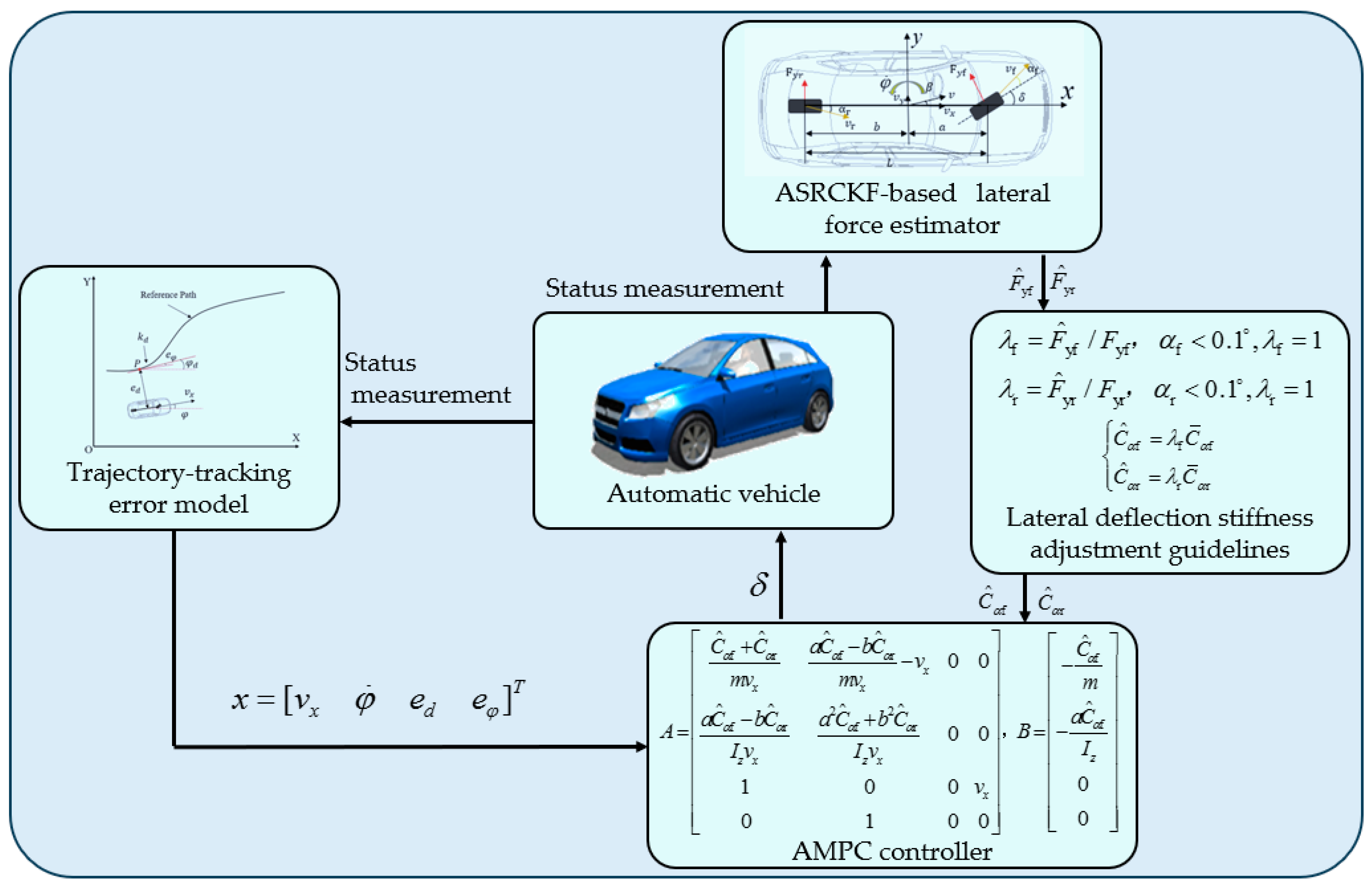
4.3. Adaptive Path-Tracking Control Framework

To obtain an adaptive MPC (AMPC) controller that considers the nonlinear tire side forces, the variables ${\overline{C}}_{\alpha \mathrm{f}}$ and ${\overline{C}}_{\alpha \mathrm{r}}$ in Equation (8) are displaced by the variables ${\widehat{C}}_{\alpha \mathrm{f}}$ and ${\widehat{C}}_{\alpha \mathrm{r}}$ in Equation (32). Figure 5 shows the proposed architecture of the path-tracing AMPC controller.

In the architecture of the path-tracing AMPC controller, the road environment information and vehicle state information obtained from the automatic vehicle system are used for trajectory planning and lateral force estimation. By combining the desired vehicle speed $v_x$ and the reference trajectory curvature $k_d$ obtained from the planning layer, the lateral distance deviation $e_d$ and heading angle deviation $e_{\phi }$ based on the vehicle-tracking error model are obtained. The estimated values of ${\widehat{F}}_{\mathrm{yf}}$ and ${\widehat{F}}_{\mathrm{yr}}$ are obtained based on the estimator designed using ASRCKF. Then, the ratio of the estimated tire forces ${\widehat{F}}_{\mathrm{yf}}$ and ${\widehat{F}}_{\mathrm{yr}}$ to the linear tire forces $F_{\mathrm{yf}}$ and $F_{\mathrm{yr}}$ is used to calculate the scaling factors ${\chi }_{\mathrm{f}}$ and ${\chi }_{\mathrm{r}}$ to adjust the lateral deflection stiffness, which in turn gives the adjusted lateral deflection stiffness values ${\widehat{C}}_{\alpha \mathrm{f}}$ and ${\widehat{C}}_{\alpha \mathrm{r}}$. Finally, by substituting the heading angle error, vehicle speed, lateral distance error, yaw rate, and the adjusted lateral stiffness values ${\widehat{C}}_{\alpha \mathrm{f}}$ and ${\widehat{C}}_{\alpha \mathrm{r}}$ into the model, the AMPC path-tracking controller is obtained. Then, the optimal front wheel steering angle $\delta$ that satisfies the constraints is calculated, enabling the lateral control of the vehicle.

5. Analysis of Simulation Results

To test the actual performance of the designed adaptive MPC controller, a common simulation platform was developed using CarSim and Simulink, which was compared with and analyzed alongside a conventional MPC controller without lateral tire stiffness correction. The main vehicle parameters involved in the experimental simulation are demonstrated in

Table 2. Technical parameters of the automatic vehicle.

Parameters	Unit	Value
$m$	kg	1413
$I_z$	kg·m2	1536.7
${\overline{C}}_{\alpha \mathrm{f}}$	N·rad−1	−112,600
${\overline{C}}_{\alpha \mathrm{r}}$	N·rad−1	−80,500
$a$	m	1.025
$\mathrm{b}$	m	1.885

. The prediction time domain is set to $N_p=25$, the control time domain is set to $N_c=15$, the sampling time is set to $T=0.02$ s, the weights of the control increment is $R=10$, the weight matrix of the output variables is $Q=\mathrm{diag} (200, 100, 100)$, and the weight coefficients of the relaxation factor is $\rho =1000$.

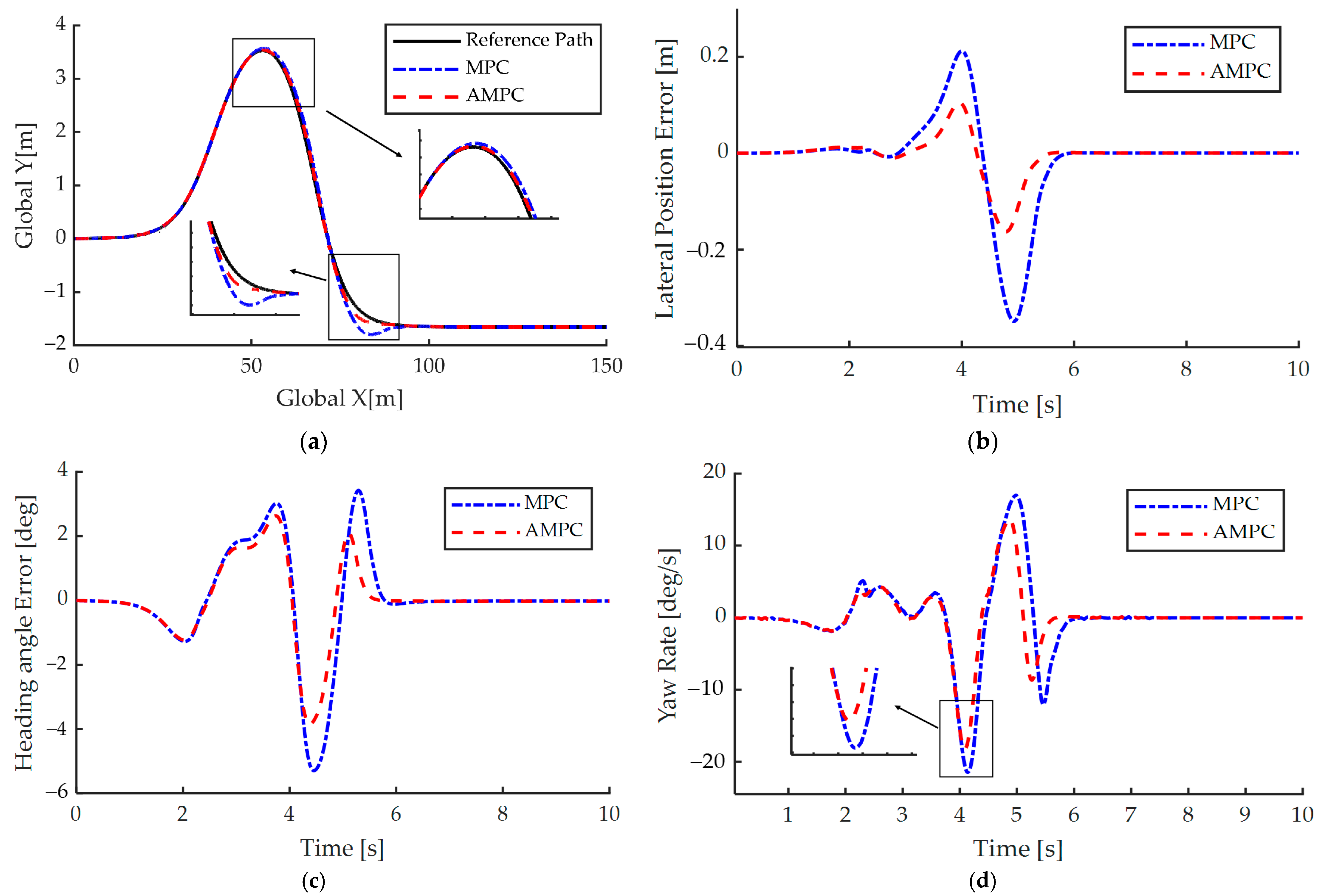
5.1. High-Adhesion Double-Shift Line Condition

The maximum road adhesion coefficient for this working condition is set to 0.8, and the vehicle speed value is 80 kph. The experimental simulation outcomes are demonstrated in Figure 6a, indicating that both controllers have achieved overall tracking of the reference trajectory. As seen in Figure 6b,c, the maximum lateral deviation and yaw angle deviation for the MPC controller are 0.3486 m and 5.295 deg, respectively. In contrast, the AMPC controller has maximum deviations of 0.1724 m and 3.855 deg, reducing them by 50.54% and 27.20%, respectively. Therefore, the AMPC controller outperforms the MPC controller in terms of overall path tracking. As seen in Figure 6d, under this condition, the vehicle yaw rate of the AMPC-based controller is less than that of the conventional MPC controller. This can reduce the lateral acceleration generated during cornering, thereby improving driving safety and ride comfort.

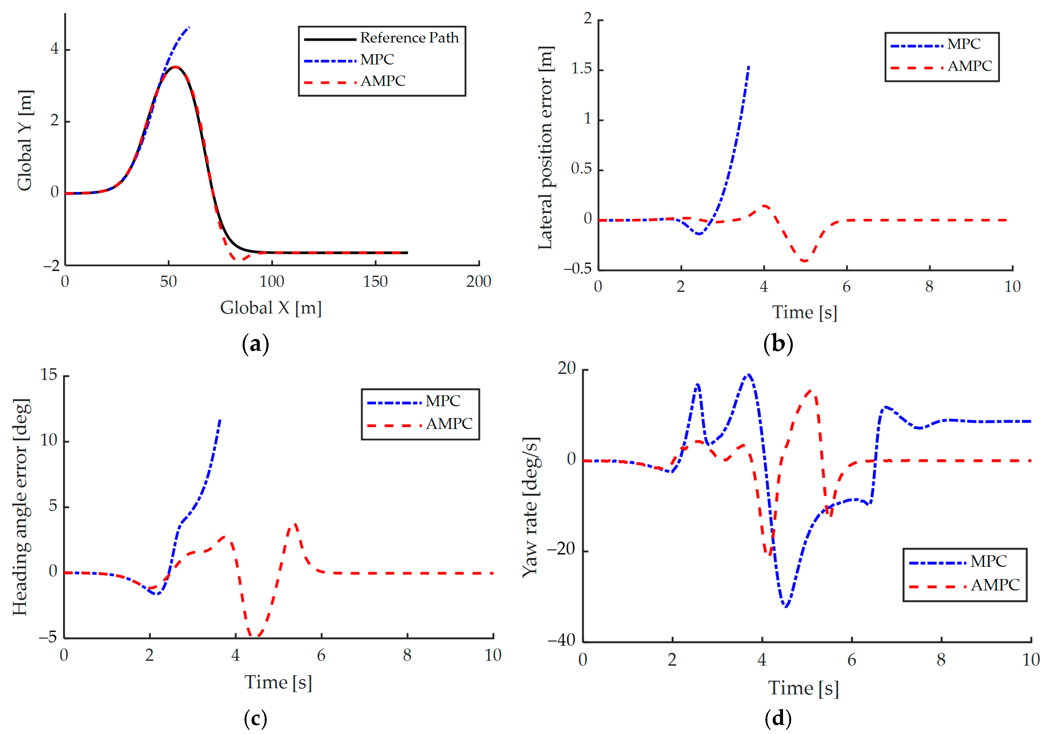
5.2. Low-Adhesion Double-Shift Line Condition

The maximum road adhesion coefficient for this working condition is 0.4, and the vehicle speed is 54 kph. The experimental simulation outcomes are demonstrated in Figure 7a, indicating that the traditional MPC controller cannot follow the reference track under this working condition. When the time exceeds 3 s, the vehicle should be turning according to the reference trajectory, but there is a phenomenon of deviation. The reason behind this is that under this working condition, the calculation of the tire’s lateral force based on linear lateral stiffness results in a significant difference from the actual lateral force. As a result, the controller is unable to calculate the steering angle of the front wheels that satisfies the driving conditions. However, the AMPC controller that incorporates adjusted lateral stiffness can still track the reference trajectory. As seen in Figure 7b,c, the lateral deviation and yaw angle deviation based on the MPC controller gradually fail to meet the path-tracking requirements after 3 s. On the other hand, the vehicle based on the AMPC controller can still suppress the lateral error and yaw angle error within 0.4989 m and 5.295 deg, respectively. The control effect is significantly superior to that of the MPC controller. In accordance with the above analysis, the AMPC controller developed in this study can significantly improve the ability of the MPC control algorithm to handle different road adhesion coefficients, which is of great importance for ensuring driving safety.

As shown in Figure 8, the solution time of each step in the whole process of the low-attachment double-shift condition test is basically maintained near 6 ms, which is much smaller than the set sampling time of 20 ms, and the experimental results show that the proposed AMPC control can guarantee the real-time performance of the optimization solution in the trajectory-tracking process. Therefore, the simulation test shows that the proposed AMPC control can meet the effectiveness and real-time performance of trajectory-tracking control and can be used in the design and optimization of intelligent vehicle control systems.

6. Conclusions

In this study, the correlation between tire lateral forces and slip angle under various vertical loads was analyzed based on the Magic tire model. A real-time tire lateral force estimator was designed using the ASRCKF algorithm, and further verification was conducted to demonstrate its effectiveness in estimating the lateral forces of the tires of a vehicle. By comparing the tire sidewall force estimated in real time with the tire force calculated using the linear tire model, a ratio was obtained and used as a proportional factor to adjust the tire lateral stiffness. Moreover, a criterion for adjusting the front and rear tire lateral stiffness was developed. Based on a vehicle tracking error model, an AMPC controller is proposed. Simulation analysis showed that under high-adhesion dual-line working conditions, the maximum lateral distance error and heading angle error are reduced by 50.54% and 27.20%, respectively. As a result, the path-tracking control effect of automatic vehicles is improved, allowing for fast and stable tracking of reference path.

The proposed AMPC algorithm has a superior adaptive ability to the road surface attachment situation and vehicle running condition and can meet the requirements of real-time tracking. The results of this research will significantly improve the stability of the traditional predictive control strategy, significantly enhance the accuracy of vehicle motion trajectory tracking, and provide a theoretical basis for improving the adaptive ability and robustness of intelligent vehicles.

In this study, the design of the controller only considered the steady state condition. The next step will consider the coupled lateral and longitudinal control of the vehicle and analyze optimal planning and control algorithms in dynamic environments.

References

1. Mu, X.; Gao, W.; Li, X.; Li, G. Coverage Path Planning for UAV Based on Improved Back-and-Forth Mode. IEEE Access 2023, 11, 114840–114854. [Google Scholar] [CrossRef]
2. Marino, R.; Scalzi, S.; Netto, M. Nested PID Steering Control for Lane Keeping in Autonomous Vehicles. Control Eng. Pract. 2011, 19, 1459–1467. [Google Scholar] [CrossRef]
3. Xu, S.; Peng, H. Design, Analysis, and Experiments of Preview Path Tracking Control for Autonomous Vehicles. IEEE Trans. Intell. Transp. Syst. 2020, 21, 48–58. [Google Scholar] [CrossRef]
4. Wang, R.; Li, Y.; Fan, J.; Wang, T.; Chen, X. A Novel Pure Pursuit Algorithm for Autonomous Vehicles Based on Salp Swarm Algorithm and Velocity Controller. IEEE Access 2020, 8, 166525–166540. [Google Scholar] [CrossRef]
5. Wang, H.; Wang, Q.; Chen, W.; Zhao, L.; Tan, D. Path Tracking Based on Model Predictive Control with Variable Predictive Horizon. Trans. Inst. Meas. Control 2021, 43, 2676–2688. [Google Scholar] [CrossRef]
6. Yakub, F.; Abu, A.; Sarip, S.; Mori, Y. Study of Model Predictive Control for Path-Following Autonomous Ground Vehicle Control under Crosswind Effect. J. Control Sci. Eng. 2016, 2016, 6752671. [Google Scholar] [CrossRef]
7. Liu, J.; Jayakumar, P.; Stein, J.L.; Ersal, T. A Study on Model Fidelity for Model Predictive Control-Based Obstacle Avoidance in High-Speed Autonomous Ground Vehicles. Veh. Syst. Dyn. 2016, 54, 1629–1650. [Google Scholar] [CrossRef]
8. Aouaouda, S.; Chadli, M.; Boukhnifer, M.; Karimi, H.R. Robust Fault Tolerant Tracking Controller Design for Vehicle Dynamics: A Descriptor Approach. Mechatronics 2015, 30, 316–326. [Google Scholar] [CrossRef]
9. Oikonomou, M.G.; Ziakopoulos, A.; Chaudhry, A.; Thomas, P.; Yannis, G. From Conflicts to Crashes: Simulating Macroscopic Connected and Automated Driving Vehicle Safety. Accid. Anal. Prev. 2023, 187, 107087. [Google Scholar] [CrossRef]
10. Nie, Z.; Jia, Y.; Wang, W.; Outbib, R. Eco-Co-Optimization Strategy for Connected and Automated Fuel Cell Hybrid Vehicles in Dynamic Urban Traffic Settings. Energy Convers. Manag. 2022, 263, 115690. [Google Scholar] [CrossRef]
11. Liu, H.; Zhang, L.; Wang, P.; Chen, H. A Real-Time NMPC Strategy for Electric Vehicle Stability Improvement Combining Torque Vectoring With Rear-Wheel Steering. IEEE Trans. Transp. Electrif. 2022, 8, 3825–3835. [Google Scholar] [CrossRef]
12. Stano, P.; Montanaro, U.; Tavernini, D.; Tufo, M.; Fiengo, G.; Novella, L.; Sorniotti, A. Model Predictive Path Tracking Control for Automated Road Vehicles: A Review. Annu. Rev. Control 2022, 55, 194–236. [Google Scholar] [CrossRef]
13. Li, H.; Luo, Y. Study on Steering Angle Input during the Automated Lane Change of Electric Vehicle; Technical Paper 2017-01–1962; SAE International: Warrendale, PA, USA, 2017. [Google Scholar] [CrossRef]
14. Liang, Y.; Li, Y.; Khajepour, A.; Zheng, L. Multi-Model Adaptive Predictive Control for Path Following of Autonomous Vehicles. IET Intell. Transp. Syst. 2020, 14, 2092–2101. [Google Scholar] [CrossRef]
15. Guo, H.; Liu, J.; Cao, D.; Chen, H.; Yu, R.; Lv, C. Dual-Envelop-Oriented Moving Horizon Path Tracking Control for Fully Automated Vehicles. Mechatronics 2018, 50, 422–433. [Google Scholar] [CrossRef]
16. Wurts, J.; Stein, J.L.; Ersal, T. Collision Imminent Steering at High Speeds on Curved Roads Using One-Level Nonlinear Model Predictive Control. IEEE Access 2021, 9, 39292–39302. [Google Scholar] [CrossRef]
17. Yakub, F.; Mori, Y. Comparative Study of Autonomous Path-Following Vehicle Control via Model Predictive Control and Linear Quadratic Control. Proc. Inst. Mech. Eng. Part J. Automob. Eng. 2015, 229, 1695–1714. [Google Scholar] [CrossRef]
18. Ji, J.; Khajepour, A.; Melek, W.W.; Huang, Y. Path Planning and Tracking for Vehicle Collision Avoidance Based on Model Predictive Control with Multiconstraints. IEEE Trans. Veh. Technol. 2017, 66, 952–964. [Google Scholar] [CrossRef]
19. Cui, Q.; Ding, R.; Wei, C.; Zhou, B. Path-Tracking and Lateral Stabilisation for Autonomous Vehicles by Using the Steering Angle Envelope. Veh. Syst. Dyn. 2021, 59, 1672–1696. [Google Scholar] [CrossRef]
20. Spielberg, N.A.; Brown, M.; Gerdes, J.C. Neural Network Model Predictive Motion Control Applied to Automated Driving with Unknown Friction. IEEE Trans. Control. Syst. Technol. 2022, 30, 1934–1945. [Google Scholar] [CrossRef]
21. Piyabongkarn, D.; Rajamani, R.; Grogg, J.A.; Lew, J.Y. Development and Experimental Evaluation of a Slip Angle Estimator for Vehicle Stability Control. IEEE Trans. Control Syst. Technol. 2009, 17, 78–88. [Google Scholar] [CrossRef]
22. Xiaoyu, L.; Nan, X.; Konghui, G. Vehicle Sideslip Angle Estimation Based on Fusion of Kinematic Method and Kinematic-geometry Method. J. Mech. Eng. 2020, 56, 121. [Google Scholar] [CrossRef]
23. Qi, G.; Yue, M.; Shangguan, J.; Guo, L.; Zhao, J. Integrated Control Method for Path Tracking and Lateral Stability of Distributed Drive Electric Vehicles with Extended Kalman Filter–Based Tire Cornering Stiffness Estimation. 2023. Available online: https://journals.sagepub.com/doi/10.1177/10775463231181635 (accessed on 11 January 2024).
24. Li, S.; Yang, Z.; Wang, X. Trajectory Tracking Control of an Intelligent Vehicle Based on T-S Fuzzy Variable Weight MPC. J. Mech. Eng. 2023, 59, 199. [Google Scholar] [CrossRef]
25. Teng, S.; Hu, X.; Deng, P.; Li, B.; Li, Y.; Ai, Y.; Yang, D.; Li, L.; Xuanyuan, Z.; Zhu, F.; et al. Motion Planning for Autonomous Driving: The State of the Art and Future Perspectives. IEEE Trans. Intell. Veh. 2023, 8, 3692–3711. [Google Scholar] [CrossRef]
26. Liu, J.; Wang, Z.; Zhang, L. Integrated Vehicle-Following Control for Four-Wheel-Independent-Drive Electric Vehicles Against Non-Ideal V2X Communication. IEEE Trans. Veh. Technol. 2022, 71, 3648–3659. [Google Scholar] [CrossRef]
27. Pacejka, H. Tire and Vehicle Dynamics; Elsevier: Amsterdam, The Netherlands, 2005. [Google Scholar]
28. Han, K.; Choi, M.; Choi, S.B. Estimation of the Tire Cornering Stiffness as a Road Surface Classification Indicator Using Understeering Characteristics. IEEE Trans. Veh. Technol. 2018, 67, 6851–6860. [Google Scholar] [CrossRef]
29. Cui, Z.; Xia, X.; Pei, X. A Modified Vehicle Following Control System on the Curved Road Based on Model Predictive Control. In Proceedings of the 2021 33rd Chinese Control and Decision Conference (CCDC), Kunming, China, 22–24 May 2021; pp. 1098–1103. [Google Scholar] [CrossRef]
30. Zhe, X.; Hailiang, C.; Ziyu, L.; Enxin, S.; Qi, S.; Shengbo, L. Lateral Trajectory Following for Automated Vehicles at Handling Limits. J. Mech. Eng. 2020, 56, 138. [Google Scholar] [CrossRef]
31. Lu, Y.; Zhu, J.; Wang, Z.; Du, N.; Zhang, J. Path Preview Tracking for Autonomous Vehicles Based on Model Predictive Control. In Proceedings of the 2022 IEEE International Conference on Unmanned Systems (ICUS), Guangzhou, China, 28–30 October 2022; pp. 405–410. [Google Scholar] [CrossRef]
32. Taghavifar, H.; Shojaei, K. Adaptive Robust Control Algorithm for Enhanced Path-Tracking Performance of Automated Driving in Critical Scenarios. Soft Comput. 2023, 27, 8841–8854. [Google Scholar] [CrossRef]
Figure 1. 2-DOF vehicle dynamics model.
Wevj 15 00095 g001
Figure 2. Path-tracking model that considers trajectory curvature.
Wevj 15 00095 g002
Figure 3. Schematic diagram of tire lateral force.
Wevj 15 00095 g003
Figure 4. Results of tire lateral force estimation. (a) Front axle lateral force. (b) Rear axle lateral force.
Wevj 15 00095 g004
Figure 5. Architecture of the path-tracing AMPC controller.
Wevj 15 00095 g005
Figure 6. Control effect of high-attachment double-shift line condition. (a) Trajectory tracking of vehicles; (b) lateral position error; (c) heading angle error; (d) yaw rate.
Wevj 15 00095 g006
Figure 7. Control effect of low-attachment double-shift line condition. The notes for (ad) are the same as in Figure 6.
Wevj 15 00095 g007
Figure 8. Time spent on each step of the solution.
Wevj 15 00095 g008