A State-of-Health Estimation Method for Lithium Batteries under Multi-Dimensional Features

Abstract

In recent years, the number of new energy vehicles has increased rapidly. The online state-of-health (SOH) prediction of lithium-ion batteries, which are core components of new energy vehicles, is crucial for maintaining vehicle safety. However, existing data-driven methods encounter challenges such as the difficult application of health feature extraction methods in practice, single feature dimensions, and complex algorithm models. This study extracted the peak height of the incremental capacity (IC) curve, constant-current charging time, and time when the battery surface temperature reaches its maximum value as health features from multiple dimensions. Furthermore, by randomly generating prey, the Pelican Optimization Algorithm (POA) fundamentally overcomes the shortcomings of traditional swarm intelligence optimization algorithms which are prone to falling into local optimal solutions. POA was introduced to optimize the Deep Extreme Learning Machine (DELM), which maximally simplified the algorithm model while ensuring accuracy. The experimental results demonstrate that this method does not require extensive historical data support. Whether applied to batteries under the same or different working conditions, all four battery groups exhibit excellent prediction results, with Root Mean Square Error (RMSE), Mean Absolute Error (MAE), and Mean Absolute Percentage Error (MAPE) values below 1.2%.

1. Introduction

Due to their high energy density, lithium-ion batteries find extensive applications in electric vehicles (EVs), electric boats, aerospace, and various other industries. Environmental friendliness, low self-discharge rate, and other advantageous properties are exhibited by lithium-ion batteries [1]. During daily use, the alternating current from the grid is converted to direct current by the inverter to charge the lithium-ion battery [2]. The continuous cycling of battery charging and discharging leads to structural changes within the battery, affecting the external environment and resulting in capacity degradation and increased internal resistance [3]. Ultimately, these phenomena result in performance degradation and affect the safety and reliability of battery operation. Therefore, it is necessary to accurately monitor the health status of lithium batteries.

There are two main methods for the health state estimation of lithium-ion batteries: model-based methods and data-driven methods. Model-based methods mainly involve constructing circuit, chemical, or mathematical models that can simulate battery aging status according to the internal or external characteristics of the battery. Model-based methods can be roughly divided into equivalent circuit models, electrochemical models, and empirical models. Equivalent circuit models simulate battery dynamic changes through combinations of electronic components. They have simple equivalent circuit structures and good parameter identification accuracy, and thus have been widely used in the field of battery health state estimation. Reference [4] uses the recursive least squares method to identify model parameters, estimates battery state through an unscented Kalman filter, and further estimates battery SOH. Reference [5] proposes a second-order equivalent circuit model that characterizes battery constant-current charging through inductance. The model’s fidelity is improved through parallel inductance, and parameter identification is performed using the non-linear least squares method. The main feature of electrochemical models is their ability to describe the internal chemical reaction characteristics of the battery, which can more accurately describe the battery’s aging mechanism and thus achieve SOH estimation. Reference [6] simplifies the two-dimensional electrochemical model of lithium-ion batteries, uses genetic algorithms to extract five characteristic parameters to characterize the battery’s aging trend, establishes a degradation model for lithium-ion batteries, and verifies its accuracy. Reference [7] establishes an electrochemical model for the battery, and experimentally demonstrates that the model can obtain high-precision estimation results. Although electrochemical models can obtain high-precision estimation results, the complex equations they contain make calculations extremely complicated and require high hardware data-processing capabilities. Empirical models generally involve establishing capacity decay models and fitting battery aging trends with empirical formulas. Empirical degradation models can model the entire life cycle of the battery, and the parameters are easy to identify, with small calculation amounts, making them suitable for online applications. Reference [8] conducts a cycle testing of batteries under different operating conditions and discharge depths, and establishes an empirical model for battery capacity decay through a large amount of empirical data, estimating the SOH of experimental batteries. However, the adaptability of empirical-degradation-model-based methods is poor. Since prior knowledge cannot consider all possible aging trends, when there is deviation in the aging trend, the estimation result will have a significant bias.

Model-based methods mainly simulate the external characteristics of batteries by constructing models, but they have poor adaptability. With the development of computer technology, data-driven SOH methods have gained more and more attention. By utilizing techniques such as machine learning and deep learning, this method estimates the SOH of lithium-ion batteries by establishing the relationship between the health features of batteries and capacity degradation [9,10]. This method does not require studying the working mechanism of the battery, but instead utilizes a large amount of data from the cycling process of lithium batteries for training. As a rule, the precision of estimation results obtained typically increases as the number of training samples increases [11]. This method’s primary research content can be categorized into two parts: health features and the estimation method for mapping the features to capacity.

1.1. Health Features

Although the battery’s voltage, current, and temperature can be monitored and measured in real time through sensors, its health status is not a directly measurable physical quantity. Therefore, in order to estimate the SOH of batteries, it is necessary to establish the mapping relationships between direct or indirect feature parameters related to SOH and these features are called battery health features. In practical applications, in order to achieve the SOH estimation of lithium-ion batteries, the selection of health features should be based on two principles. One approach is to select representative health features that characterize the aging status of the battery. Second, the selected health features should be easily obtained online and better facilitate the online application of battery SOH estimation in practical use. Generally, charging and discharging data of the battery are used to extract health features [12,13,14]. The charging and discharging cycles of the battery will cause certain changes in the voltage, current, and temperature curves during the charging and discharging process. These changes have an inherent connection with battery capacity degradation and can reflect the degree of battery aging. Under experimental conditions, the charge and discharge conditions of the battery are relatively simple, making feature extraction easy. In practical applications, the discharge stage of the battery has complex and variable operating conditions, which makes feature extraction difficult. Therefore, in practical applications, health features are more easily extracted from the charging-stage data of the battery, which is beneficial for realizing the online estimation of battery SOH.

1.2. Developing Methods for Mapping between Features and Capacity Estimation

Data-driven algorithms can effectively mine potential feature information in the battery capacity degradation process and use intelligent algorithms, neural networks, and other offline training historical battery data to test and estimate the SOH of batteries online, thereby achieving an accurate estimation of the SOH of lithium-ion batteries. Data-driven methods include time-series methods [15,16,17,18], statistical data-driven methods [19], and machine learning methods [20,21,22,23,24,25]. By learning a large amount of historical data and feature patterns, machine learning algorithms can accurately predict the state of battery health. Compared to traditional physics-based methods, machine learning methods are better able to capture small changes and non-linear relationships within the battery. Additionally, machine learning methods can adaptively adjust based on the actual usage of the battery, improving the accuracy of estimation results. This method can handle various types and brands of batteries, and adapt to various working conditions and environmental changes.

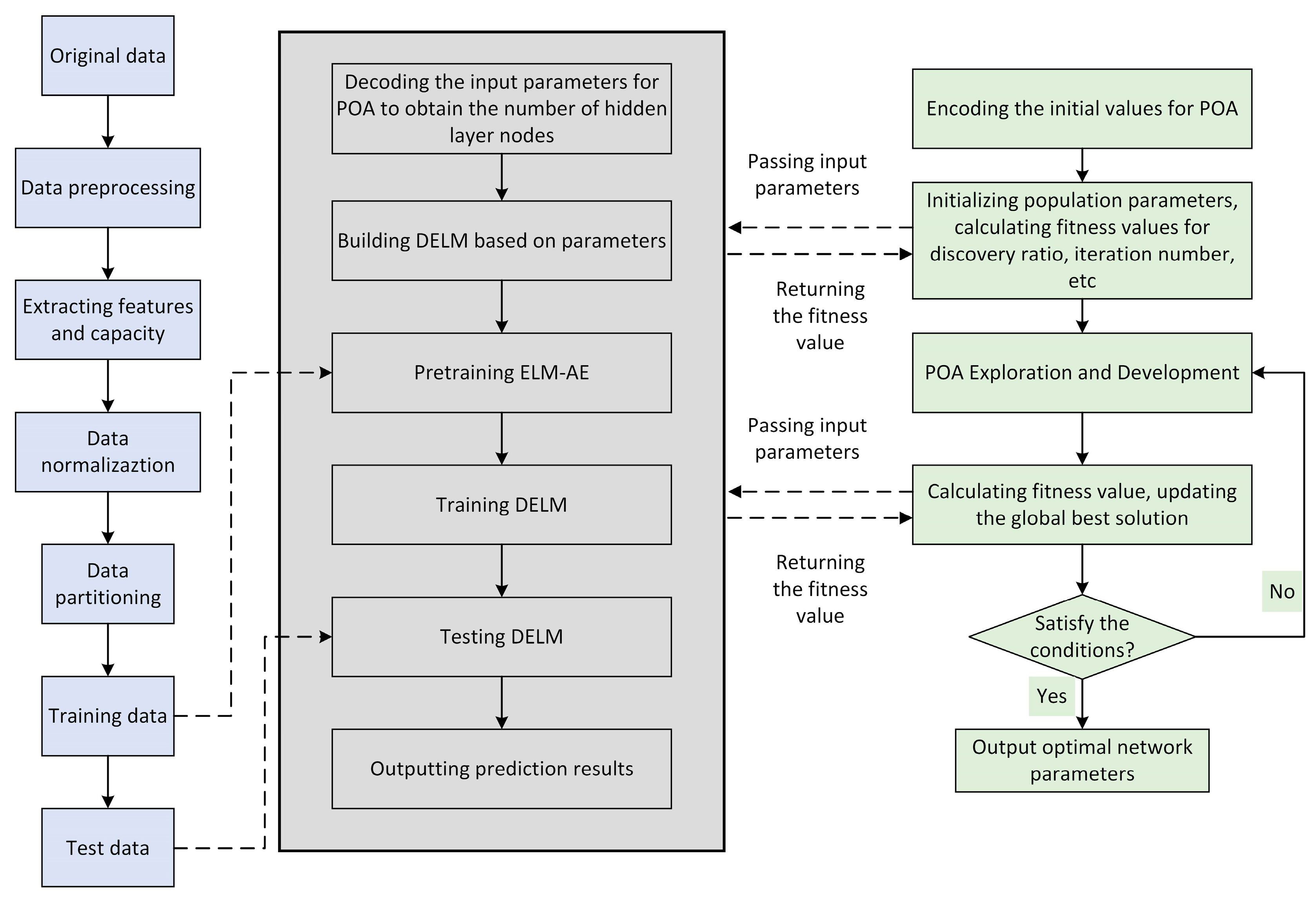
To address the issues of weak usability in health feature extraction, single feature dimensionality, and complex algorithm models in existing data-driven methods, this study proposes an innovative approach. This study first extracts three features from the charging data to indirectly characterize battery capacity degradation: IC peak value, time to reach peak temperature, and constant-current charging time. Considering the limitation of randomly given connection weights and thresholds between the input layer and hidden layer in the traditional DELM algorithm, the POA algorithm is introduced to optimize the model structure. Unlike other swarm intelligence optimization algorithms, POA searches for prey by randomly generating prey, enhancing its global search capability. The random generation of prey solves the problem of excessive reliance on mutation coefficients in other algorithms to escape local optima.

The structure of this paper is as follows: Section 2 provides an overview of the process of establishing the POA-DELM model. Section 3 focuses on the analysis and extraction of health features. Section 4 presents the estimation results and discusses them. Finally, Section 5 summarizes the main conclusions.

2. POA-DELM Model

2.1. POA

Optimization involves the examination of multiple solutions to a problem and selecting the optimal one. In fact, problems with multiple feasible solutions are considered optimization problems. Decision variables, constraints, and objective functions are the key elements in modeling an optimization problem [26]. Generally, methods for solving optimization problems can be divided into two categories: deterministic and stochastic techniques [27]. When dealing with complex optimization problems characterized by non-derivative, non-convex, high-dimensional, and discontinuous objective functions, deterministic methods encounter difficulties. In contrast, stochastic methods can overcome these challenges by utilizing random searches within the solution space of the problem, instead of relying on derivatives and gradients of the objective function. This allows stochastic methods to provide suitable solutions to optimization problems. Amongst stochastic methods, population-based optimization algorithms are considered highly effective.

The Pelican Optimization Algorithm, hereafter referred to as POA, is a new algorithm proposed by Pavel in 2022. Pelicans are natural hunters that feed on fish and collaborate as a group during their hunting process. The pelican team patrols the prey from a height of over ten meters, and once they spot the prey, they swiftly swoop down towards it. When they reach the surface, they use their wings to drive the prey into a narrow area and then swallow it into their throat pouches. The global search ability of POA is enhanced by randomly generated fish locations, unlike other algorithms that rely on the coefficient of variation to overcome the lack of local optimization search ability. This fundamental difference sets the Pelican Optimization Algorithm apart from other algorithms. POA follows the steps outlined below:

(1)

Initialization parameters: Set the spatial dimension S of the independent variable to be optimized. $C_{max}$ represents the maximum number of iterations, and P represents the size of the population.

(2)

Construct the fitness function and update the optimal position of the initial pelican population Xpest = X(0) and the fitness of the current position Fbest = F(Xpest).

(3)

During the exploration phase, pelican populations patrol prey over the water, randomly generating prey locations and continuously updating pelican population locations.

$$x_{i,j}^{Q1}=\{\begin{array}{ll}{x}_{i,j}+\mathrm{rand}\cdot \left(Q_j-I\cdot x_{i,j}\right),\hfill & F_Q<F_i\hfill \\ x_{i,j}+\mathrm{rand}\cdot \left(x_{i,j}-Q_j\right),\hfill & \mathrm{else}\hfill \end{array}$$

(1)

where the updated position of the exploration phase is denoted as $x_{i,j}^{Q1}$, indicating the position of the jth dimension in the ith generation. $Q_j$ represents the position of the prey on the jth dimension, while $F_Q$ represents the value of the objective function associated with the prey, and I denotes a random number, either 1 or 2, which determines whether the individual moves a greater distance into a new exploration area when I = 2. Therefore, POA’s capacity to thoroughly search the solution space is influenced by the parameter I. Once the pelican finishes searching for prey, the fitness of the new position is compared to the old position, and the optimal position is updated to the position with the lowest fitness. This way, the pelican moves towards the optimal area.

$$x_i=\{\begin{array}{ll}{x}_i^{Q1}\hfill & F_i^{Q1}<F_i\hfill \\ x_i\hfill & \mathrm{else}\hfill \end{array}$$

(2)

where $X_i^{Q1}$ denotes the updated state of the ith pelican, while $F_i^{Q1}$ represents the objective function value obtained during the exploration phase.

(4)

During the development phase, the pelican’s wings will spread, and the fish will be driven into the pelican’s throat pouch, which is mathematically modelled as follows:

$$x_{i,j}^{Q2}=x_{i,j}+\mathrm{R}\cdot \left(1-\frac{t}{C_{max}}\right)\cdot (2\cdot \mathrm{rand}{}^{-1})\cdot x_{i,j}$$

(3)

where $x_{i,j}^{Q2}$ represents the position of the ith generation in the jth dimension based on the updated position of the development phase. R is a constant equal to 0.2, and $\mathrm{R}\cdot \left(1-\frac{t}{C_{max}}\right)$ represents the radius of the neighborhood of $x_{i,j}$, where $t/C_{max}$ denotes the iteration process.

After completing the development phase, the fitness of the new position is compared with that of the old position, and the best position at this point is updated to the position with the lowest fitness.

$$x_i=\{\begin{array}{ll}{x}_i^{Q2}\hfill & F_i^{Q2}<F_i\hfill \\ x_i,\hfill & \mathrm{else}\hfill \end{array}$$

(4)

where $x_i^{Q2}$ represents the position of the ith generation during the exploration stage, and $F_i^{Q2}$ represents the fitness score of the pelican.

(5)

Update the global optimal position of the pelican to Xgpest = X(1), and the global optimal fitness of the current position to Fgbest = F(Xgbosx). Then, repeat steps (3) and (4) until the maximum number of iterations is reached.

2.2. DELM

The Extreme Learning Machine (ELM) structure, as shown in Figure 1, improves the overall training speed by reducing learning time and network complexity through random weight selection. However, its single hidden layer structure may not capture all the features of high-dimensional and large-scale data samples. ELM-AE is an autoencoder, whose structure is shown in Figure 2, and it learns sample feature representation in an unsupervised way by mapping inputs to hidden layer feature vectors and reconstructing feature vectors into original inputs through a decoder. In contrast to ELM’s single hidden layer structure, DELM initializes weights using ELM-AE, as shown in Figure 3, and can more effectively handle high-dimensional and large-scale data and improve feature learning efficiency by introducing multi-layer structures and autoencoders. From a structural perspective, DELM can be viewed as connecting multiple ELMs. Compared to ELM, DELM can more comprehensively capture sample features and enhance the accuracy of handling high-dimensional inputs. DELM learns layer by layer through ELM-AE in an unsupervised way, and connects to the regression layer for supervised training without requiring a simultaneous adjustment of system parameters.

DELM offers improved accuracy and versatility compared to ELM. However, it is worth noting that the input layer weights in the pre-training phase of ELM-AE are orthogonal random matrices generated randomly. During the pre-training process of ELM-AE, only the weight parameters of the output layer are adjusted using least squares, while the weights of the input layer remain unchanged. Therefore, the random input weights of each ELM-AE will have an impact on the final prediction performance of DELM. Therefore, optimizing the model’s parameters becomes crucial in enhancing the prediction performance of DELM.

2.3. POA Optimization of DELM Model Building

DELM introduces the inclusion of regularization terms to prevent overfitting, which is a shared disadvantage with ELM neural networks. Both DELM and ELM encounter the challenge of randomly assigning connection weights and thresholds between the input and hidden layers. This randomness can result in prolonged training times, susceptibility to local optima, and the risk of overfitting or underfitting the model. To address this issue, it is proposed to use a POA-optimized DELM neural network to adjust the connection weights and thresholds between the input layer and the hidden layer. Figure 4 illustrates the overall framework for estimating the SOH of lithium batteries.

The detailed steps are outlined as follows:

(1)

The original dataset is preprocessed, followed by the extraction of health features and capacity decline data for each cycle. Finally, the normalized dataset is split into two sets: a training set and a test set.

(2)

The POA algorithm utilizes encoding techniques to initialize the parameters, which include the spatial dimension of independent variables, the population size, and the maximum number of iterations, which are all important parameters.

(3)

The POA algorithm receives input parameters from DELM, The number of hidden layer nodes is derived by decoding the aforementioned information. This value is then used to calculate the fitness value, which serves as the initial fitness value for the POA algorithm.

(4)

The DELM model is constructed and pre-trained using the training set. Additionally, during this stage, the objective function’s fitness value is computed.

(5)

The fitness values of the objective function are compared, and the resulting optimal fitness value is updated. The pelican population patrols its prey near the water’s surface, with the position of the fish randomly generated and the position of the pelican population subsequently adjusted. The pelicans then spread their wings to drive the prey into their throat pouches.

(6)

Determine whether the iteration conditions are satisfied. If the conditions are met, terminate the loop, output the optimal network parameters, and proceed to step (7). Otherwise, repeat step (5).

(7)

The optimal network parameters obtained from the output are used to initialize the DELM. Subsequently, the test set is inputted into the POA-DELM model to generate predictions.

3. Data Preprocessing and Feature Engineering

Based on the international IEEE standard, battery health indicators are typically divided into two categories: internal resistance and capacity. When the internal resistance of the battery doubles its initial value or when the current available capacity reduces to 70% of the initial value, the battery should be considered as scrapped and disposed of. For the purpose of this paper, capacity is chosen as the indicator of battery health status.

$$\mathrm{SOH}=\frac{Q_r}{Q_n}\times 100\%$$

(5)

In Equation (5), $Q_r$ represents the actual maximum usable capacity of the lithium-ion battery, while $Q_n$ represents the nominal usable capacity stated on the lithium-ion battery nameplate.

3.1. Health Characteristic Selection

Currently, the health factor for estimating battery health state is typically extracted from directly measurable voltage, current, and temperature profiles. Mathematically, in the constant-current charging mode, the IC value represents the quantity of battery power supplied during a continuous voltage increment, and is calculated using the following formula:

$$\mathrm{IC}=\frac{dQ}{dU}=I\frac{dt}{dU}$$

(6)

In this equation, Q represents charge, U represents voltage, and t represents sampling time. During the constant-current charging stage, the value of I can be treated as a constant, and the value of the IC curve is negatively correlated with the rate of change of voltage over time. In practical applications, the peaks of the IC curve are influenced by the voltage differential interval. If the voltage difference interval is too large, the peak features of the IC curve for cycles with significant aging will be lost. On the other hand, if the differential voltage interval is too small, not only will the Pearson coefficient between peak features and SOH be reduced, but it will also increase the computational burden. Therefore, after repeated tests, a differential voltage interval of 30 millivolts was chosen. Additionally, due to interference from measurement noise, it is not possible to directly obtain the peak values of the IC curve. Kalman filtering is used to denoise the original IC curve. Based on Figure 5, it can be observed that as the cycle number increases, the peaks of the IC curve significantly decrease. Thus, the peaks of the IC curve can serve as health indicators.

During the charging process, batteries generate a considerable amount of heat. Figure 6 presents the curves of temperature change over time for batteries subjected to different cycles. The battery temperature rises during the constant-current charging stage and then decreases during the constant-voltage charging stage. The time required to reach the highest temperature during the constant-current charging stage can be used as an indicator of overall performance, as the battery dissipates unrecoverable heat during this stage. As the number of cycles increases, the time required to reach peak temperature typically decreases. Therefore, the time required to reach peak temperature can be used as a health indicator metric.

Because the majority of battery charging methods include two stages, constant-current charging and constant-voltage charging, the time required for the battery to reach the desired voltage during the charging process can also serve as a health factor. As the battery ages, it often reaches the desired voltage earlier during the constant-current charging stage. Figure 7 illustrates the variation in battery charging current during different cycles. It can be observed that as the battery ages, the constant-current charging time significantly decreases. Taking the B5 battery as an example, in the 20th cycle, it takes approximately 3350 s to reach the designated charging cutoff voltage, while in the 140th cycle, it only takes about 1730 s. Therefore, the constant-current charging time can also be used as one of the indicators for assessing the battery’s health condition.

A visual analysis of the three features in this paper is performed through Figure 5, Figure 6 and Figure 7. It can be observed from the figures that the values of the three features gradually decrease with the deepening of battery aging. Finally, the IC peak value, the time to reach the highest temperature, and the constant-current charging time are named HF1, HF2, and HF3, respectively. In order to illustrate the degree of correlation with SOH more intuitively, these three features are normalized and shown in Figure 8 with respect to SOH. It can be observed that all three selected features exhibit a strong correlation with SOH.

3.2. Examining the Relationship between Specific Health Characteristics and SOH

Calculating the Pearson correlation coefficient is a method to assess the linear relationship between two variables. Specifically, in order to calculate the correlation between the extracted features and battery capacity, the ratio of covariance to standard deviation is used to compute the Pearson correlation coefficient. When the correlation between the selected features and capacity approaches 1 or −1, it indicates a strong correlation between them. The formula for calculating the Pearson correlation coefficient is as follows:

$$\mathrm{Pearson}=\frac{{{\displaystyle \sum }}_{i=1}^n\left(x_i-\overline{x}\right)\left(y_i-\overline{y}\right)}{\sqrt{{{\displaystyle \sum }}_{i=1}^n{\left(x_i-\overline{x}\right)}^2}\sqrt{{{\displaystyle \sum }}_{i=1}^n{\left(y_i-\overline{y}\right)}^2}}$$

(7)

Table 1. The Pearson correlation coefficients between the chosen features and battery capacity.

Batteries	B0005	B0006	B0007	B0018
HF1	0.9967	0.9964	0.9929	0.9854
HF2	0.9976	0.9865	0.9835	0.9818
HF3	0.9980	0.9952	0.9970	0.9909

presents the Pearson correlation coefficients between the extracted health features and the SOH of the four lithium-ion batteries. A Pearson correlation coefficient greater than 0.95 signifies an exceptionally strong correlation between the features and the capacity. By analyzing Table 1, it is evident that the selected features exhibit a remarkably strong correlation with the SOH.

4. Analysis of Experimental Results

Before analyzing and discussing the experimental results, a comparison was made between the existing online SOH evaluation techniques for lithium-ion batteries and the work presented in this paper, as shown in

Table 2. Comparison of this paper’s methodology with existing online SOH assessment techniques for lithium-ion batteries.

Existing Online SOH Evaluation Techniques for Lithium-ion Batteries		Characteristics
Equivalent circuit models		It has poor adaptability, and its estimation results depend heavily on the parameter identification of the model and the performance of the filtering algorithm.
Data-driven methods	Estimating the SOH using discharge data.	It is challenging to control the actual discharge conditions.
	Estimating the SOH using a single-scale feature.	The estimation results are unstable.
	Estimating the SOH using multi-scale features.	The charging mode of lithium-ion batteries is constant, and the estimation results of multi-scale features are more stable and accurate.

.

This paper utilizes data from the NASA Li-ion battery dataset (B0005, B0006, B0007, and B0018) tested by the NASA PCoE Research Center [28]. The dataset comprises 18,650 batteries on which charge–discharge and impedance tests were conducted at an ambient temperature of 24 °C. The maximum cut-off voltage was set to 4.2 V, and the battery was charged with a constant current of 1.5 A until it reached the maximum cut-off voltage limit. Then, it was switched to constant-voltage charging, which ended when the charging current dropped to 20 mA. The experiment was terminated when the capacity dropped to 70% of its initial capacity. B0005, B0006, and B0007 were subjected to 166 charge/discharge cycles each, while B0018 underwent 130 charge/discharge cycles. The experimental setup included an Intel(R) Core(TM) i7-7500U CPU processor @ 2.70 GHz 2.90 GHz and 12 GB of operating memory, Windows 10 Standard Edition 64-bit operating system, and MATLAB as the experimental software with version R2020b.

4.1. Experiment 1

The training set for battery B0005 consists of the first 70% of the cycles, while the test set comprises the remaining 30% of the cycles. As depicted in Figure 9, the fitness value of the POA-DELM algorithm tends to be stable in less than 30 iterations. Figure 10 displays the prediction results for battery B0005, and the predicted results for batteries 5, 6, 7, and 18 are presented in

Table 3. NASA test errors for cells 5, 6, 7, and 18 When the training set was set to 70%.

	Methodology of This Paper				POA-ELM				ELM
	5	6	7	18	5	6	7	18	5	6	7	18
RMSE (%)	0.57	1.00	0.44	0.94	1.25	1.76	1.76	1.20	1.30	2.67	2.38	1.99
MAE (%)	0.41	0.75	0.38	0.64	0.93	1.38	1.38	0.97	1.52	2.06	2.00	1.54
MAPE (%)	0.60	1.20	0.52	0.92	1.40	2.25	1.55	1.40	1.30	3.38	2.78	2.25

.

The level of agreement between the forecasted and actual SOH values for battery B0005 was measured to be 0.9214. Under the same testing conditions with an equal proportion of training set, the predictive performance of the three algorithms is shown in Figure 11, Figure 12, Figure 13 and Figure 14. In comparison to other algorithms, Table 2 provides a comprehensive analysis of the RMSE percentage, MAE percentage, and MAPE for the POA-DELM algorithm.

Table 3 illustrates the notable reduction in estimation error achieved by the POA-DELM algorithm compared to ELM and POA-ELM. To further demonstrate the accuracy of this approach,

Table 4. Percentage reduction in error of our method vs. the other two methods.

	POA-ELM	ELM
RMSE (%)	43.2	62.5
MAE (%)	45.7	63.6
MAPE (%)	46.7	64.5

highlights the percentage reduction in estimation error achieved by this paper’s method as compared to the other two algorithms used on the B0006 cell.

4.2. Experiment 2

To validate that the proposed method does not rely on a large amount of training data, only the first 50% of data from battery groups B5, B6, B7, and B18 was used as the training set, and the remaining 50% of the data was designated as the testing set. The experimental results for different algorithms on the four battery groups are presented in Figure 15, Figure 16, Figure 17 and Figure 18. From the figures, it can be observed that the ELM algorithm accurately tracks the initial degradation trend of SOH. However, as the capacity inflection point appears, it fails to accurately predict the subsequent cycles’ SOH values. On the other hand, POA-ELM is not influenced by the capacity inflection point, but its prediction accuracy exhibits an unstable distribution of errors. The proposed method in this paper, on the other hand, demonstrates higher accuracy in tracking the SOH degradation trend and capturing capacity inflection points, with a more stable distribution of errors.

The errors of the proposed method and the other two algorithms on the four battery groups are shown in

Table 5. NASA test errors for cells 5, 6, 7, and 18 When the training set was set to 50%.

	Methodology of This Paper				POA-ELM				ELM
	B5	B6	B7	B18	B5	B6	B7	B18	B5	B6	B7	B18
RMSE (%)	0.57	0.92	0.47	0.77	1.25	2.92	1.33	1.24	3.37	3.13	2.90	3.38
MAE (%)	0.41	0.77	0.4	0.67	0.93	1.38	0.98	0.93	3.02	2.83	2.55	3.02
MAPE (%)	0.60	1.16	0.54	0.97	1.40	3.27	1.351	1.40	4.43	4.2	3.48	4.43

. It can be observed that neither the proposed method nor the POA-ELM algorithm exhibits significantly larger errors due to the reduction of the training set samples to 50%. The performance of the proposed method and the POA-ELM algorithm in terms of RMSE, MAE, and MAPE is comparable to when the training set samples accounted for 70% of the total samples. However, the ELM algorithm is particularly sensitive to a reduction in the number of samples in the training set, with its error metrics being approximately 1.62 times higher compared to when the training set accounted for 70% of the total samples. Furthermore, although the POA-ELM algorithm is also unaffected by the decrease in training set samples, its error metrics are all greater than those of the POA-DELM algorithm.

4.3. Experiment 3

In practical scenarios, different batteries may undergo distinct aging processes and exhibit varied performance in different temperature environments. To account for these variations, the B0006 battery was employed as the training set, whereas the B0005 battery was utilized as the test set. Similarly, the B0018 battery served as the training set, while the B0007 battery was designated as the test set. As depicted in Figure 19 and Figure 20, even when trained on one set of batteries and tested on another set, the proposed method achieved satisfactory results, with an overall error rate below 1% and a coefficient of determination exceeding 0.99.

Table 6. NASA test errors for cells 5 and 7.

	B5	B7
RMSE (%)	0.88	0.64
MAE (%)	0.73	0.51
MAPE (%)	0.93	0.60
R2 (%)	99.63	99.57

presents the prediction error metrics for the B0005 and B0007 batteries.

5. Conclusions

This research proposes a technique for the online SOH assessment of lithium-ion batteries. Firstly, three features are extracted from the battery charging data: IC peak, time to reach peak temperature, and constant-current charging time. These features characterize the degradation state of the battery capacity. Considering the limitations of the traditional DELM algorithm that relies on randomly assigned connection weights and thresholds between the input and hidden layers, this paper introduces the concept of randomly generated prey to address this issue. The randomly generated prey enhances the global search capability of the POA algorithm and overcomes the dependency on prey variability in other algorithms. Furthermore, the introduction of the POA algorithm avoids the drawback of relying solely on the coefficient of variation to avoid local optima and optimizes the model structure. Compared with POA-ELM, the RMSE, MAE, and MAPE of the proposed method are reduced by 43.2%, 45.7%, and 46.7%, respectively. Compared with ELM, the RMSE, MAE, and MAPE are reduced by 62.5%, 63.6%, and 64.5%, respectively. The final simulation results demonstrate that the proposed model has the capability of online SOH measurement, high estimation accuracy, good generalization performance, and the ability to track capacity regeneration phenomena. Among all the comparison models, the proposed method achieves the highest accuracy and exhibits the most stable error distribution. Although the method proposed in this study has a lower requirement for the number of training samples, it achieves higher accuracy in estimating SOH. However, the feature extraction in this research is based on complete charging data. In practical engineering scenarios, sometimes only fragmented charging data can be obtained. Further research is needed to explore how to accurately estimate SOH based on fragmented charging data of lithium-ion batteries.

References

1. Tang, X.; Zou, C.; Wik, T.; Yao, K.; Xia, Y.; Wang, Y.; Yang, D.; Gao, F. Run-to-run control for active balancing of lithium iron phosphate battery packs. IEEE Trans. Power Electron. 2020, 35, 1499–1512. [Google Scholar] [CrossRef]
2. Havrlík, M.; Libra, M.; Poulek, V.; Kourím, P. Analysis of Output Signal Distortion of Galvanic Isolation Circuits for Monitoring the Mains Voltage Waveform. Sensors 2022, 22, 7769. [Google Scholar] [CrossRef] [PubMed]
3. Zhang, J.; Lee, J. A review on prognostics and health monitoring of Li-ion battery. J. Power Sources 2011, 196, 6007–6014. [Google Scholar] [CrossRef]
4. Xu, Z.; Wang, J.; Lund, P.D.; Zhang, Y. Co-estimating the state of charge and health of lithium batteries through combining a minimalist electrochemical model and an equivalent circuit model. Energy 2022, 240, 122815. [Google Scholar] [CrossRef]
5. Yang, J.; Xia, B.; Huang, W.; Fu, Y.; Mi, C. Online state-of-health estimation for lithium-ion batteries using constant-voltage charging current analysis. Appl. Energy 2018, 212, 1589–1600. [Google Scholar] [CrossRef]
6. Xiong, R.; Tian, J.; Mu, H.; Wang, C. A systematic model-based degradation behavior recognition and health monitoring method for lithium-ion batteries. Appl. Energy 2017, 207, 372–383. [Google Scholar] [CrossRef]
7. Huang, M.; Kumar, M. Electrochemical Model-Based Aging Characterization of Lithium-Ion Battery Cell in Electrified Vehicles. In Proceedings of theASME 2018 Dynamic Systems and Control Conference, Atlanta, GA, USA, 30 September–3 October 2018. [Google Scholar]
8. Wang, J.; Liu, P.; Hicks-Garner, J.; Sherman, E.; Soukiazian, S.; Verbrugge, M.; Tataria, H.; Musser, J.; Fianamore, P. Cycle-life model for graphite-LiFePO4 cells. J. Power Sources 2011, 196, 3942–3948. [Google Scholar] [CrossRef]
9. Andre, D.; Appel, C.; Soczka-Guth, T.; Sauer, D. Advanced mathematical methods of SOC and SOH estimation for lithium-ion batteries. J. Power Sources 2013, 224, 20–27. [Google Scholar] [CrossRef]
10. Fan, Y.; Xiao, F.; Li, C.; Yang, G.; Tang, X. A novel deep learning framework for state of health estimation of lithium-ion battery. J. Energy Storage 2020, 32, 101741. [Google Scholar] [CrossRef]
11. Khumprom, P.; Yodo, N. A data-driven predictive prognostic model for lithium-ion batteries based on a deep learning algorithm. Energies 2019, 12, 660. [Google Scholar] [CrossRef]
12. Yang, D.; Zhang, X.; Pan, R.; Wang, Y.; Chen, Z. A novel Gaussian process regression model for state-of-health estimation of lithium-ion battery using charging curve. J. Power Sources 2018, 384, 387–395. [Google Scholar] [CrossRef]
13. Li, Q.; Li, D.; Zhao, K.; Wang, L.; Wang, K. State of health estimation of lithium-ion battery based on improved ant lion optimization and support vector regression. J. Energy Storage 2022, 50, 104215. [Google Scholar] [CrossRef]
14. Lipu, M.; Hannan, M.; Hussain, A.; Hoque, M.; Ker, P.; Saad, M.; Ayob, A. A review of state of health and remaining useful life estimation methods for lithium-ion battery in electric vehicles: Challenges and recommendations. J. Clean. Prod. 2018, 205, 115–133. [Google Scholar] [CrossRef]
15. Park, M.; Lee, J.; Kim, B. SOH Estimation of Li-Ion Battery Using Discrete Wavelet Transform and Long Short-Term Memory Neural Network. Appl. Sci. 2022, 12, 3996. [Google Scholar] [CrossRef]
16. Zhou, Y.; Huang, M. Lithium-ion batteries remaining useful life prediction based on a mixture of empirical mode decomposition and ARIMA model. Microelectron. Reliab. 2016, 65, 265–273. [Google Scholar] [CrossRef]
17. Khaleghi, S.; Hosen, M.; Karimi, D.; Behi, H.; Beheshti, S.; Van Mierlo, J.; Berecibar, M. Developing an online data-driven approach for prognostics and health management of lithium-ion batteries. Appl. Energy 2022, 308, 118348. [Google Scholar] [CrossRef]
18. Li, Y.; Luo, L.; Zhang, C.; Liu, H. State of Health Assessment for Lithium-Ion Batteries Using Incremental Energy Analysis and Bidirectional Long Short-Term Memory. World Electr. Veh. J. 2023, 14, 188. [Google Scholar] [CrossRef]
19. Peng, Y.; Hou, Y.; Song, Y.; Pang, J.; Liu, D. Lithium-ion battery prognostics with hybrid Gaussian process function regression. Energies 2018, 11, 1420. [Google Scholar] [CrossRef]
20. Wang, Z.; Zeng, S.; Guo, J.; Qin, T. State of health estimation of lithium-ion batteries based on the constant voltage charging curve. Energy 2019, 167, 661–669. [Google Scholar] [CrossRef]
21. Ma, C.; Zhai, X.; Wang, Z.; Tian, M.; Yu, Q.; Liu, L.; Liu, H.; Wang, H.; Yang, X. State of health prediction for lithium-ion batteries using multipleview feature fusion and support vector regression ensemble. Int. J. Mach. Learn. Cybern. 2019, 10, 2269–2282. [Google Scholar] [CrossRef]
22. Chen, Z.; Sun, M.; Shu, X.; Xiao, R.; Shen, J. Online state of health estimation for lithium-ion batteries based on support vector machine. Appl. Sci. 2018, 8, 925. [Google Scholar] [CrossRef]
23. Song, Y.; Liu, D.; Hou, Y.; Yu, J.; Peng, Y. Satellite lithium-ion battery remaining useful life estimation with an iterative updated RVM fused with the KF algorithm. Chin. J. Aeronaut. 2018, 31, 31–40. [Google Scholar] [CrossRef]
24. Jian, P. Prediction study on the degeneration of lithium-ion battery based on fuzzy inference system. Mod. Phys. Lett. B 2017, 31, 1740083. [Google Scholar]
25. Saha, B.; Goebel, K.; Christophersen, J. Comparison of prognostic algorithms for estimating remaining useful life of batteries. Trans. Inst. Meas. Control 2015, 31, 293–308. [Google Scholar] [CrossRef]
26. Ray, T.; Liew, K.M. Society and civilization: An optimization algorithm based on the simulation of social behavior. IEEE Trans. Evol. Comput. 2003, 7, 386–396. [Google Scholar] [CrossRef]
27. Stroe, D.; Schaltz, E. Lithium-ion battery state-of-health estimation using the incremental capacity analysis technique. IEEE Trans. Ind. Appl. 2020, 56, 678–685. [Google Scholar] [CrossRef]
28. Saha, B.; Goebel, K. Battery Data Set. NASA Ames Prognostics Data Repository, Moffett Field. Available online: http://ti.arc.nasa.gov/project/prognostic-datarepository (accessed on 20 March 2023).
Figure 1. ELM structure diagram.
Wevj 15 00068 g001
Figure 2. ELM-AE structure diagram.
Wevj 15 00068 g002
Figure 3. DELM structure diagram.
Wevj 15 00068 g003
Figure 4. Overall block diagram of SOH estimation for lithium batteries.
Wevj 15 00068 g004
Figure 5. Different cycle IC curves.
Wevj 15 00068 g005
Figure 6. Different cycle temperature curves.
Wevj 15 00068 g006
Figure 7. Different cycle current curves.
Wevj 15 00068 g007
Figure 8. The trend of SOH normalized with three features.
Wevj 15 00068 g008
Figure 9. Convergence curve of fitness value.
Wevj 15 00068 g009
Figure 10. Test set prediction results.
Wevj 15 00068 g010
Figure 11. The forecasting outcomes of the B5 battery for the three algorithms.
Wevj 15 00068 g011
Figure 12. The forecasting outcomes of the B6 battery for the three algorithms.
Wevj 15 00068 g012
Figure 13. The forecasting outcomes of the B7 battery for the three algorithms.
Wevj 15 00068 g013
Figure 14. The forecasting outcomes of the B18 battery for the three algorithms.
Wevj 15 00068 g014
Figure 15. The B5 battery was subjected to the prediction analysis of the three algorithms.
Wevj 15 00068 g015
Figure 16. The B6 battery was subjected to the prediction analysis of the three algorithms.
Wevj 15 00068 g016
Figure 17. The B7 battery was subjected to the prediction analysis of the three algorithms.
Wevj 15 00068 g017
Figure 18. The B18 battery was subjected to the prediction analysis of the three algorithms.
Wevj 15 00068 g018
Figure 19. Battery B0005 SOH prediction results and errors.
Wevj 15 00068 g019
Figure 20. Battery B0007 SOH prediction results and errors.
Wevj 15 00068 g020