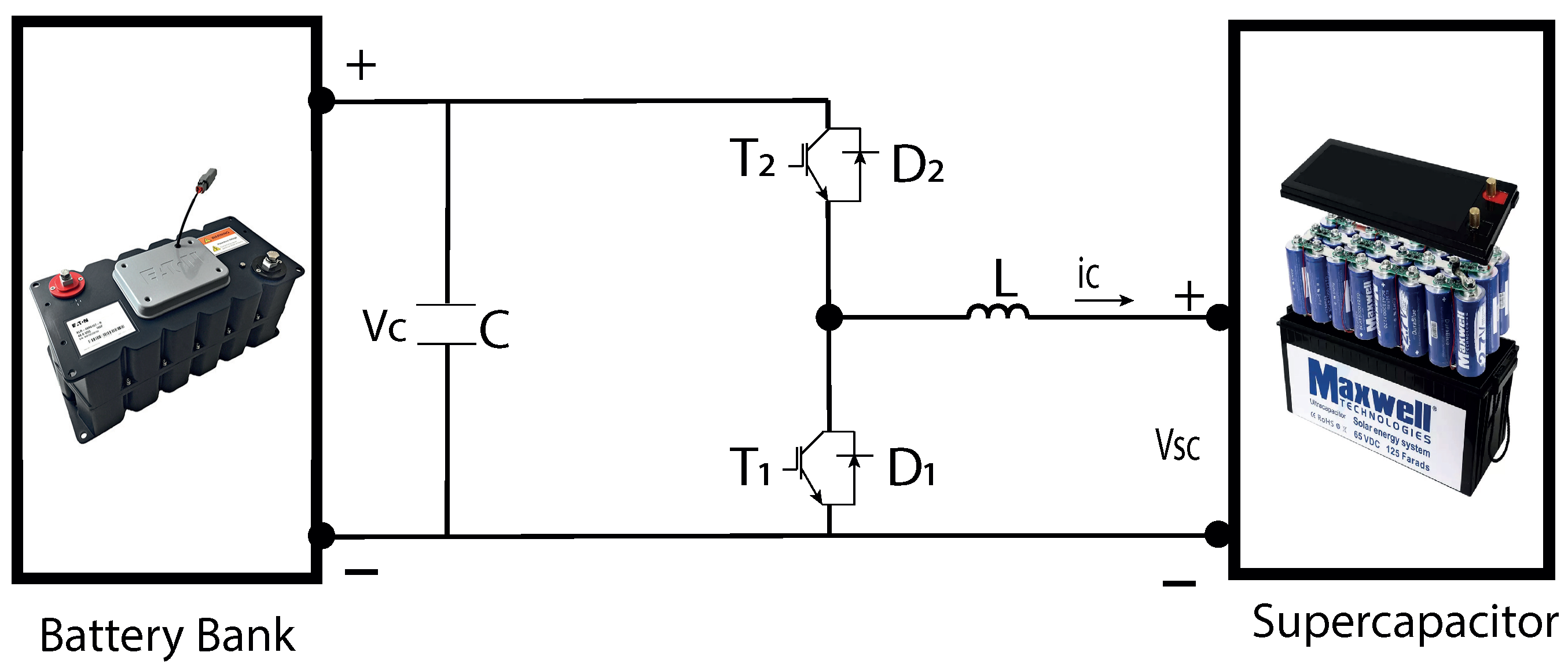
Figure 1.
DC buck-boost converter circuit.
Figure 1.
DC buck-boost converter circuit.
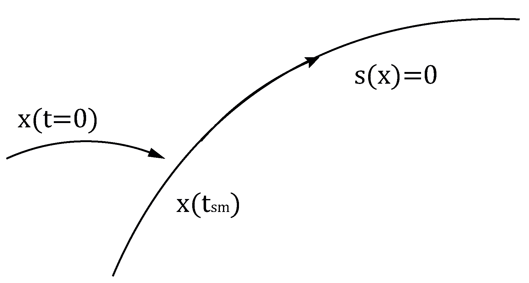
Figure 2.
Continuous-time system trajectory when SMC is applied.
Figure 2.
Continuous-time system trajectory when SMC is applied.
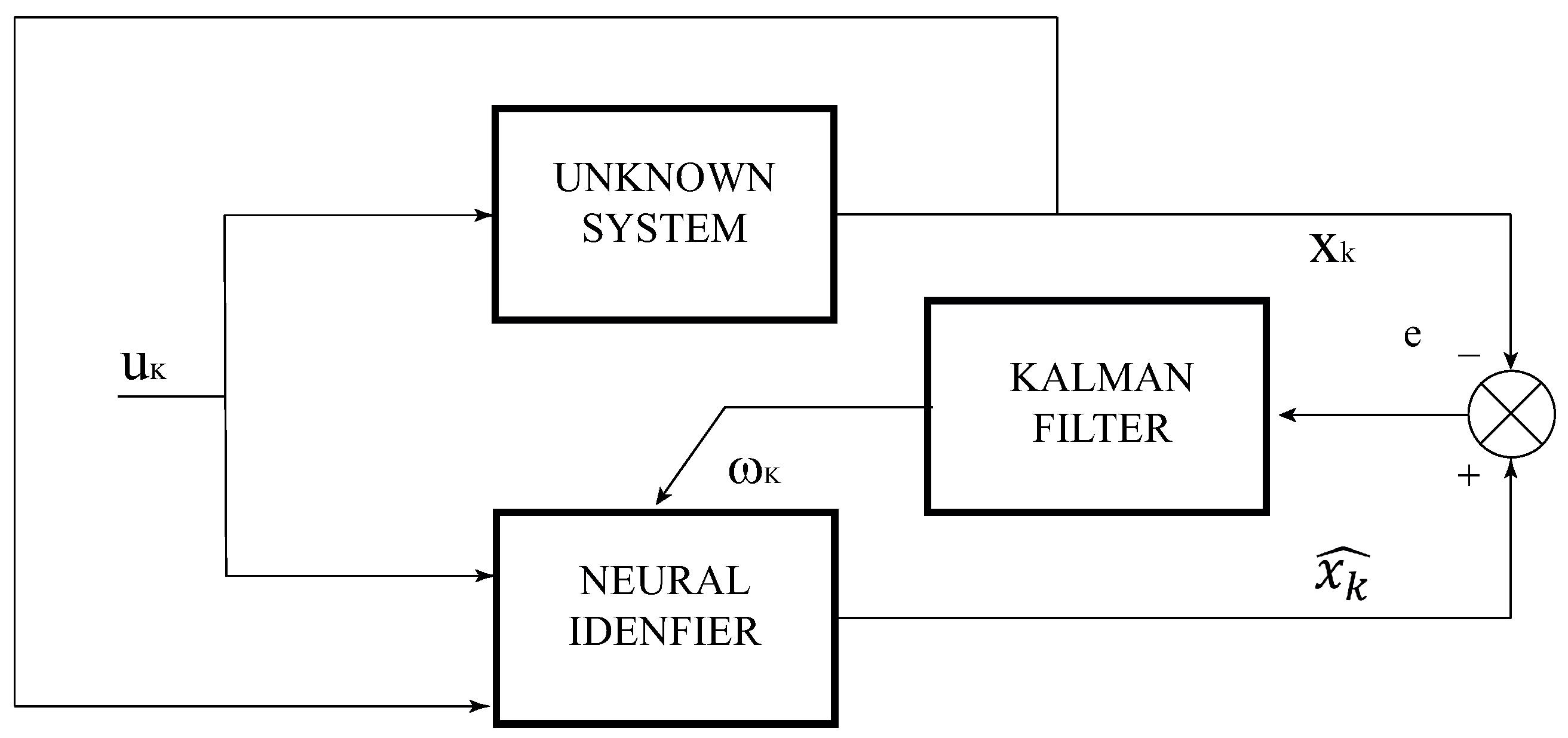
Figure 3.
Scheme of a RHONN identifier.
Figure 3.
Scheme of a RHONN identifier.
Figure 4.
Neural identification representation strategy.
Figure 4.
Neural identification representation strategy.
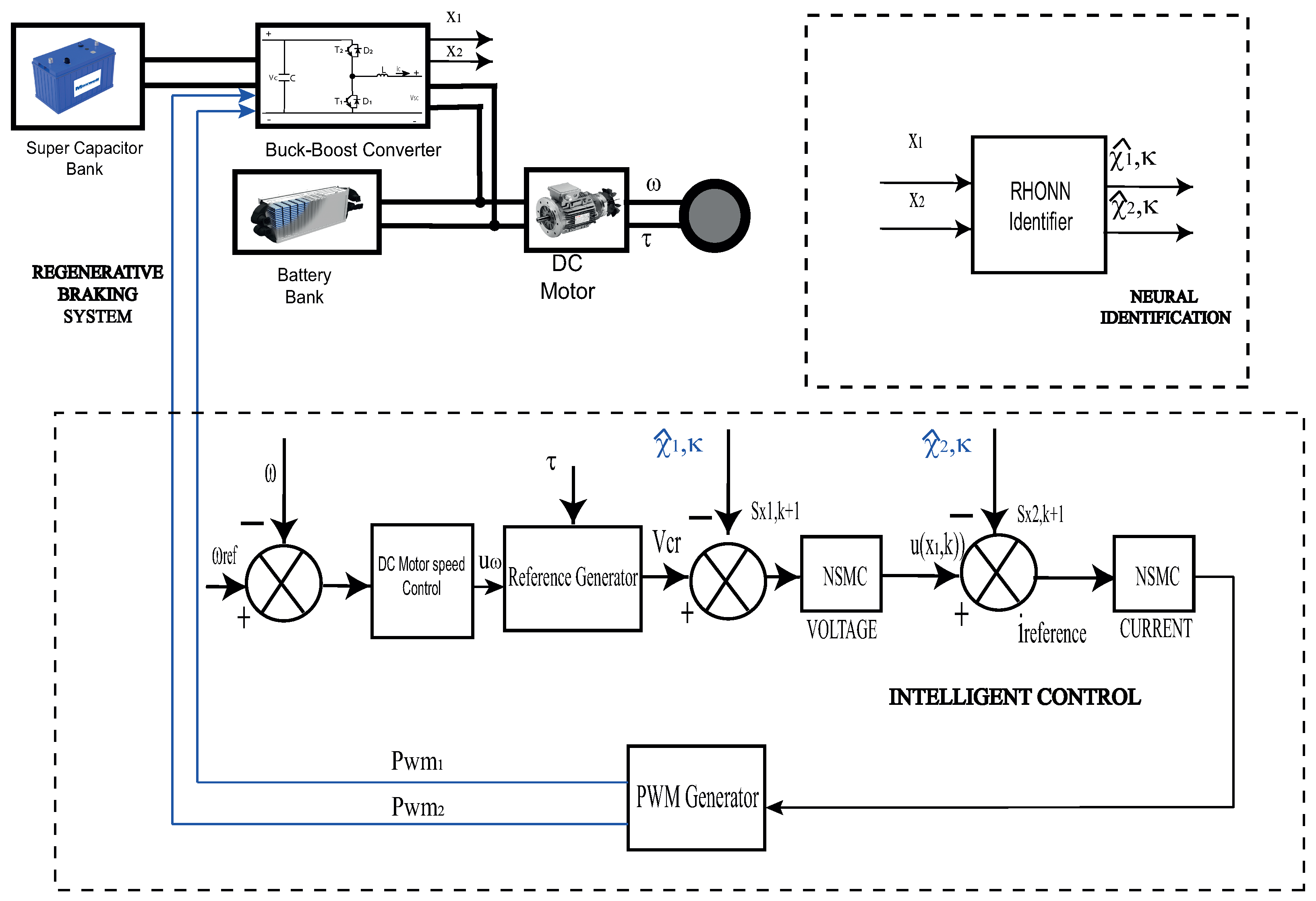
Figure 5.
Regenerative braking system control representation.
Figure 5.
Regenerative braking system control representation.
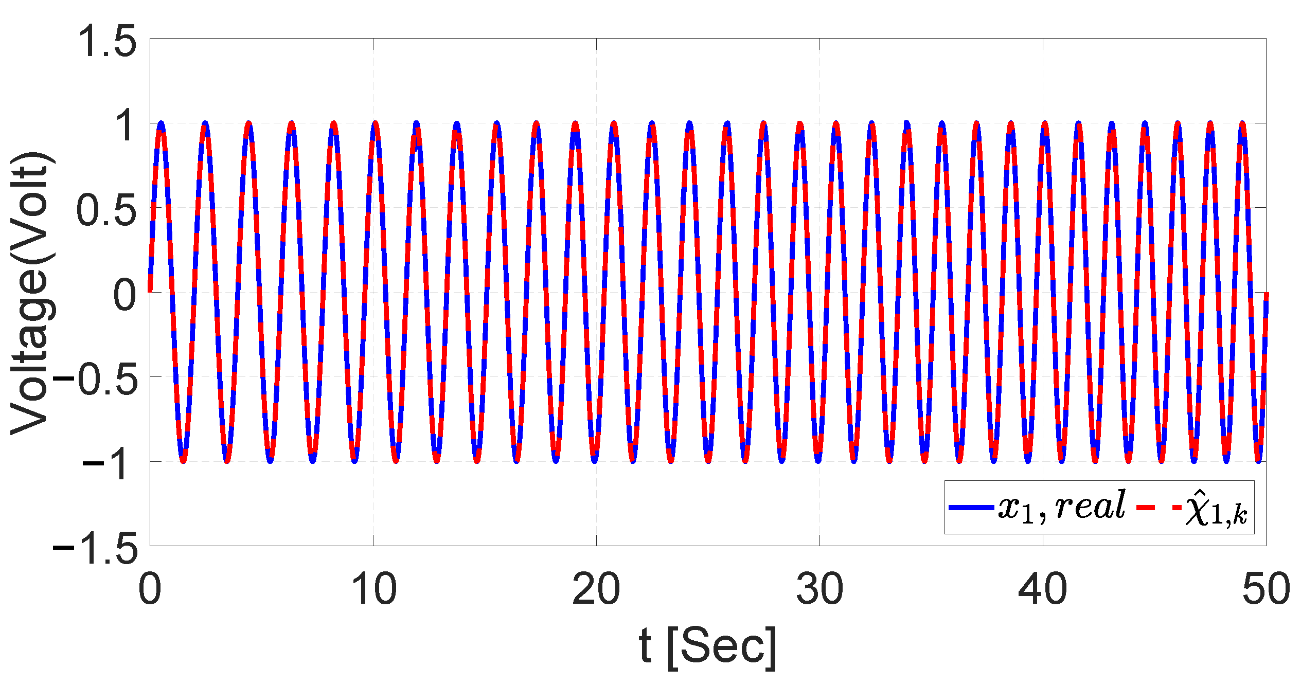
Figure 6.
Chirp signal identification for voltage with UKF.
Figure 6.
Chirp signal identification for voltage with UKF.
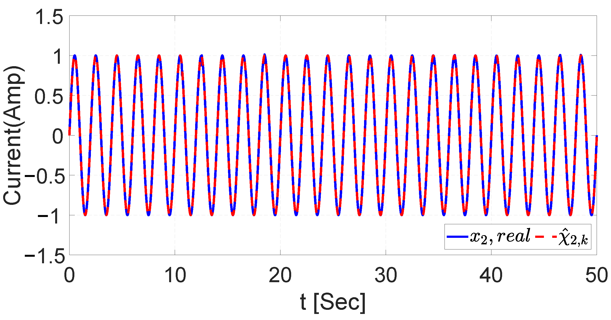
Figure 7.
Chirp signal identification for current with UKF.
Figure 7.
Chirp signal identification for current with UKF.
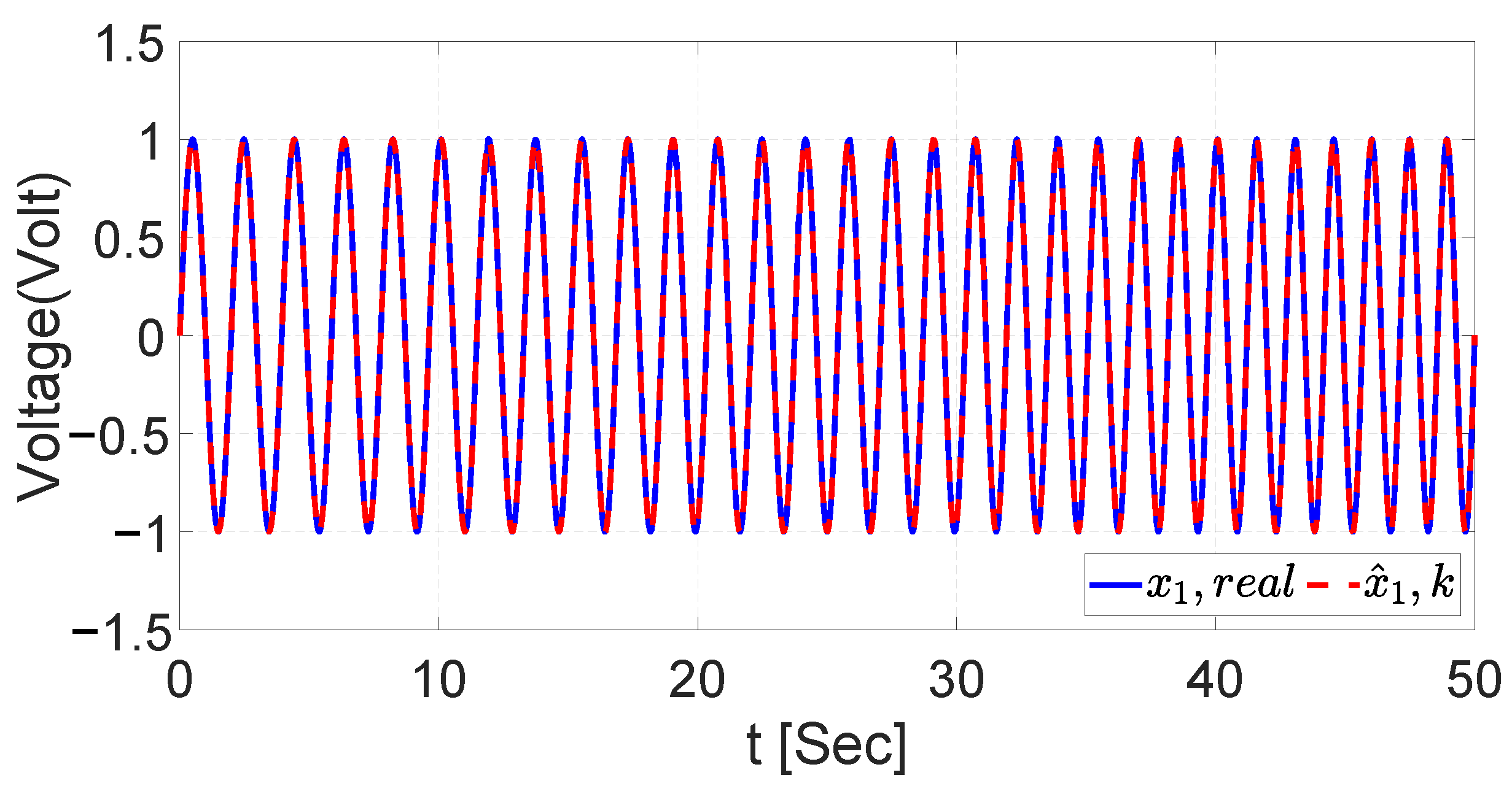
Figure 8.
Chirp signal identification for voltage with EKF.
Figure 8.
Chirp signal identification for voltage with EKF.
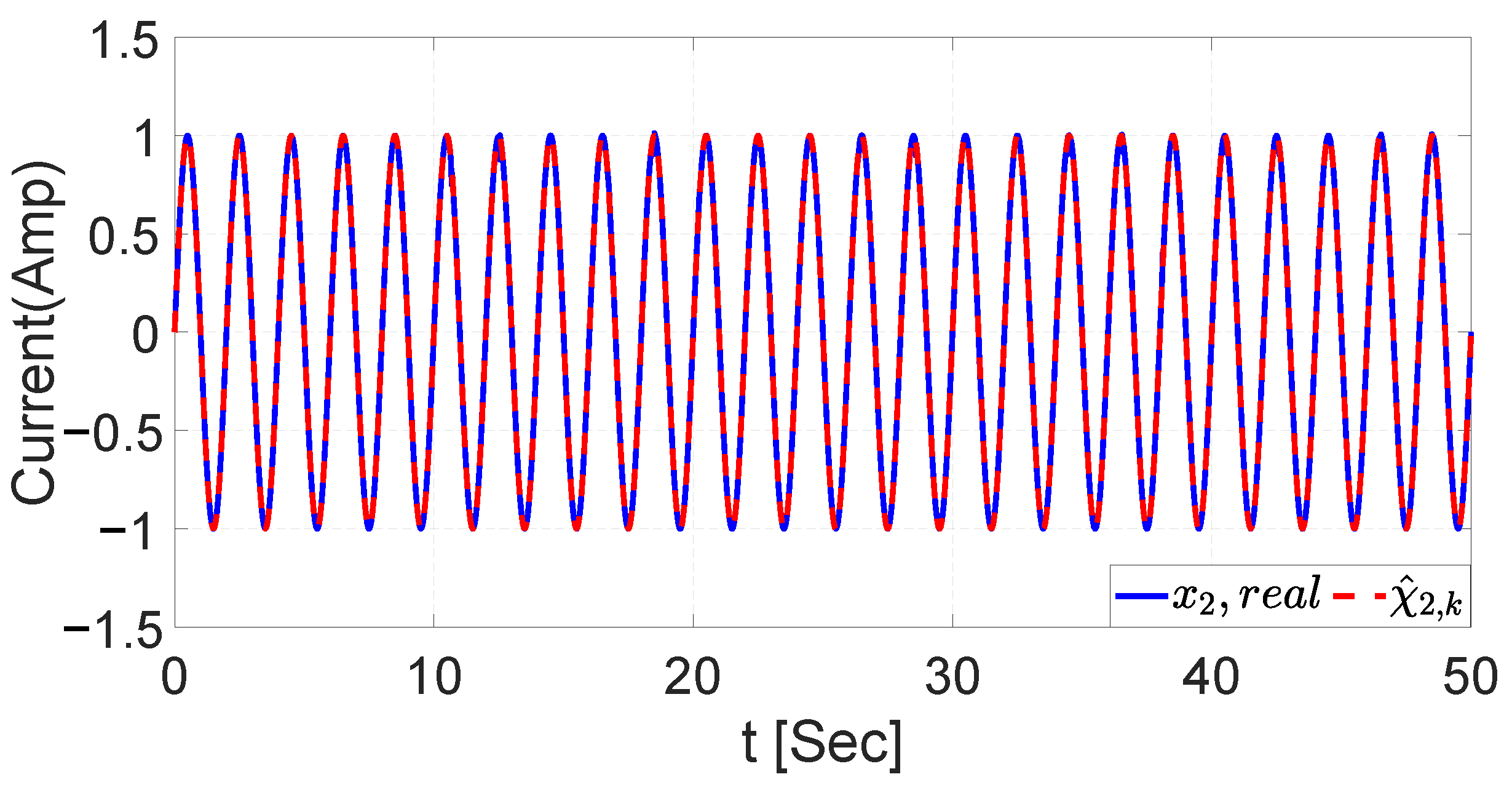
Figure 9.
Chirp signal identification for current with EKF.
Figure 9.
Chirp signal identification for current with EKF.
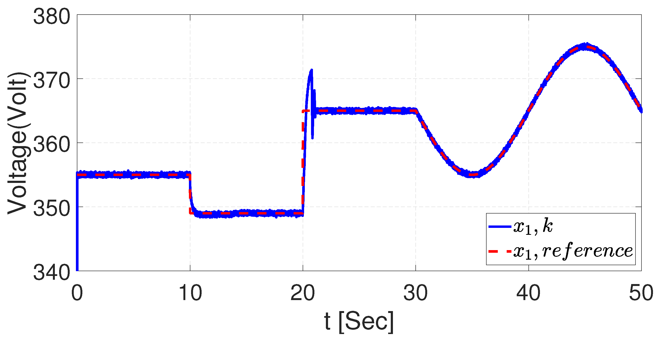
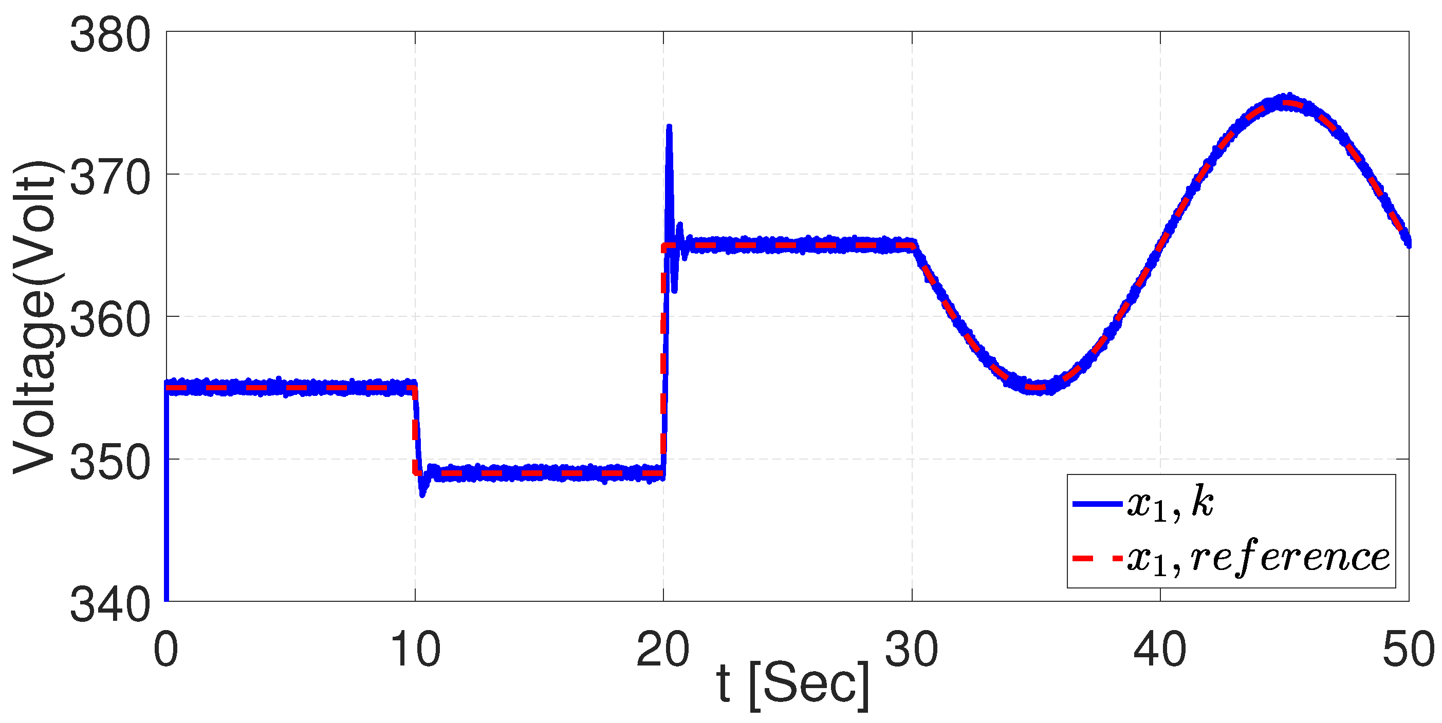
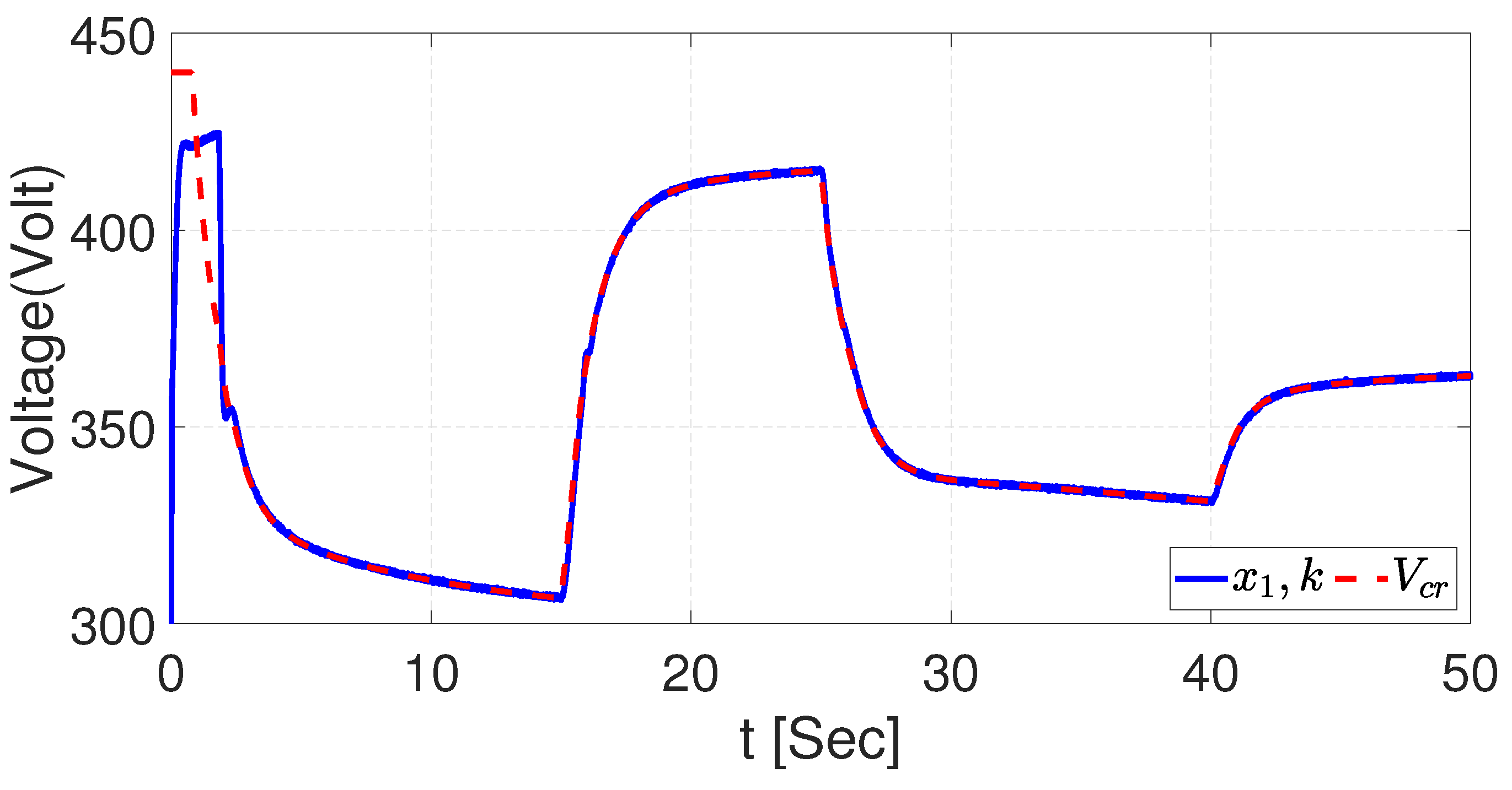
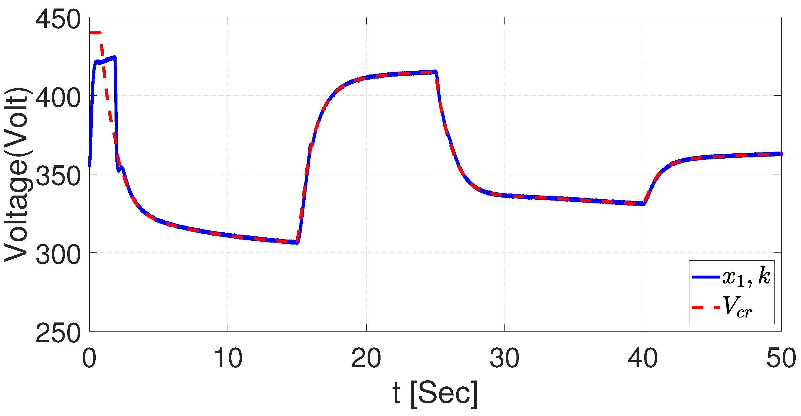
Figure 10.
Voltage dynamics trajectory tracking with UKF.
Figure 10.
Voltage dynamics trajectory tracking with UKF.
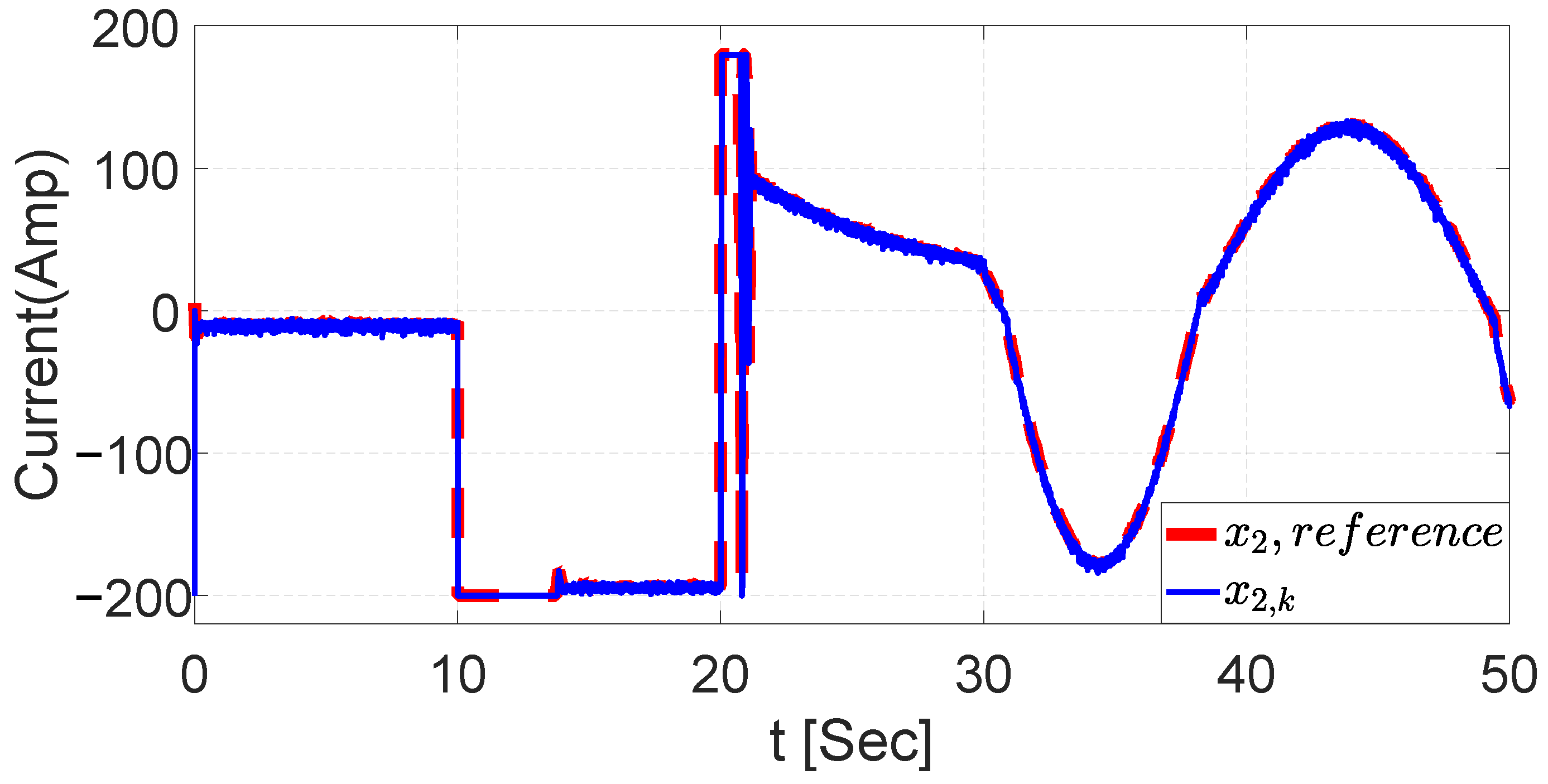
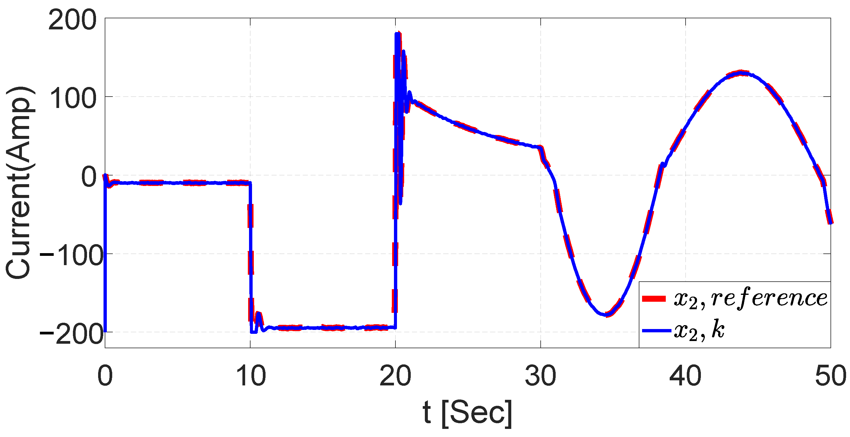
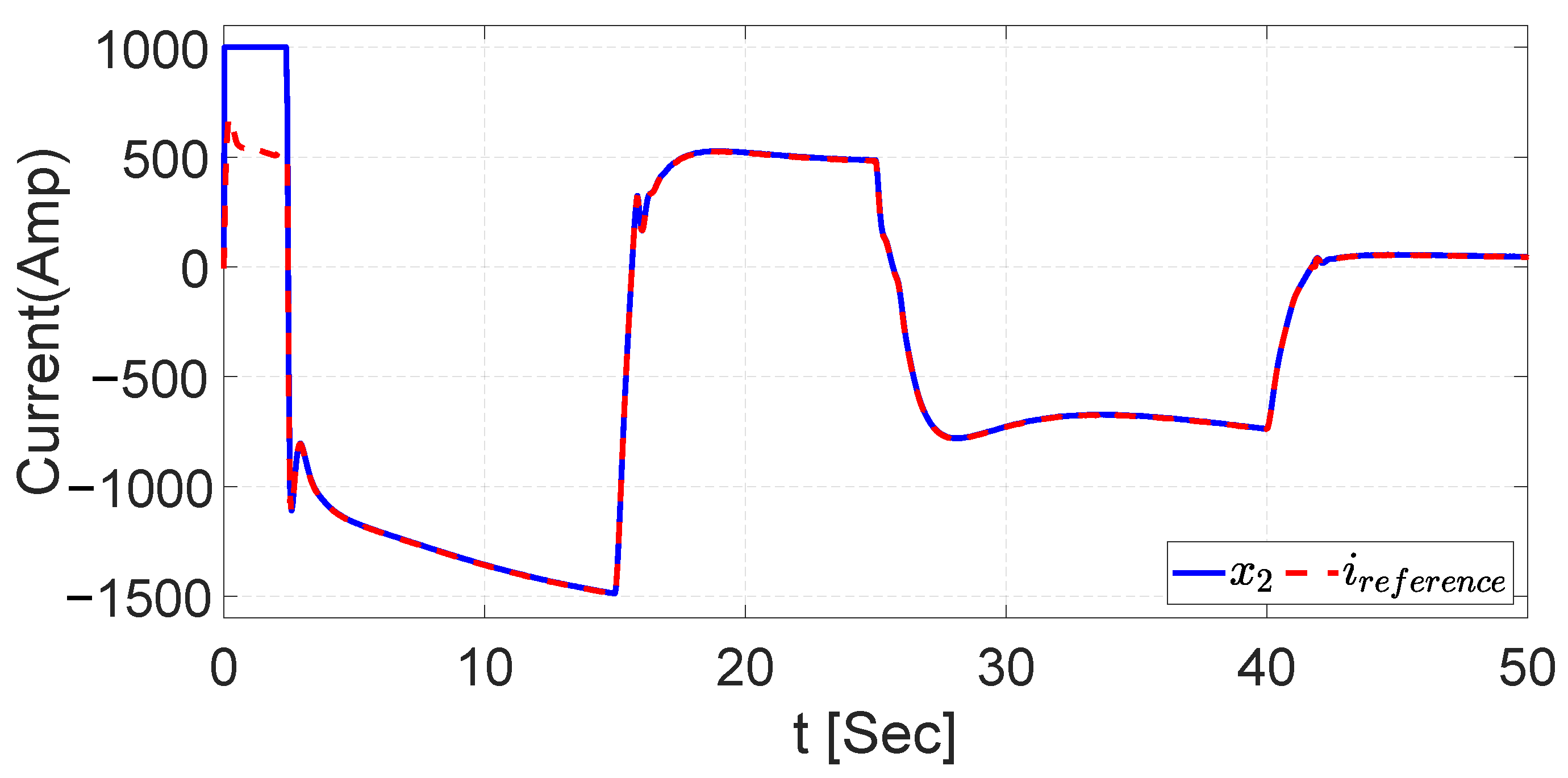
Figure 11.
Current dynamics trajectory tracking with UKF.
Figure 11.
Current dynamics trajectory tracking with UKF.
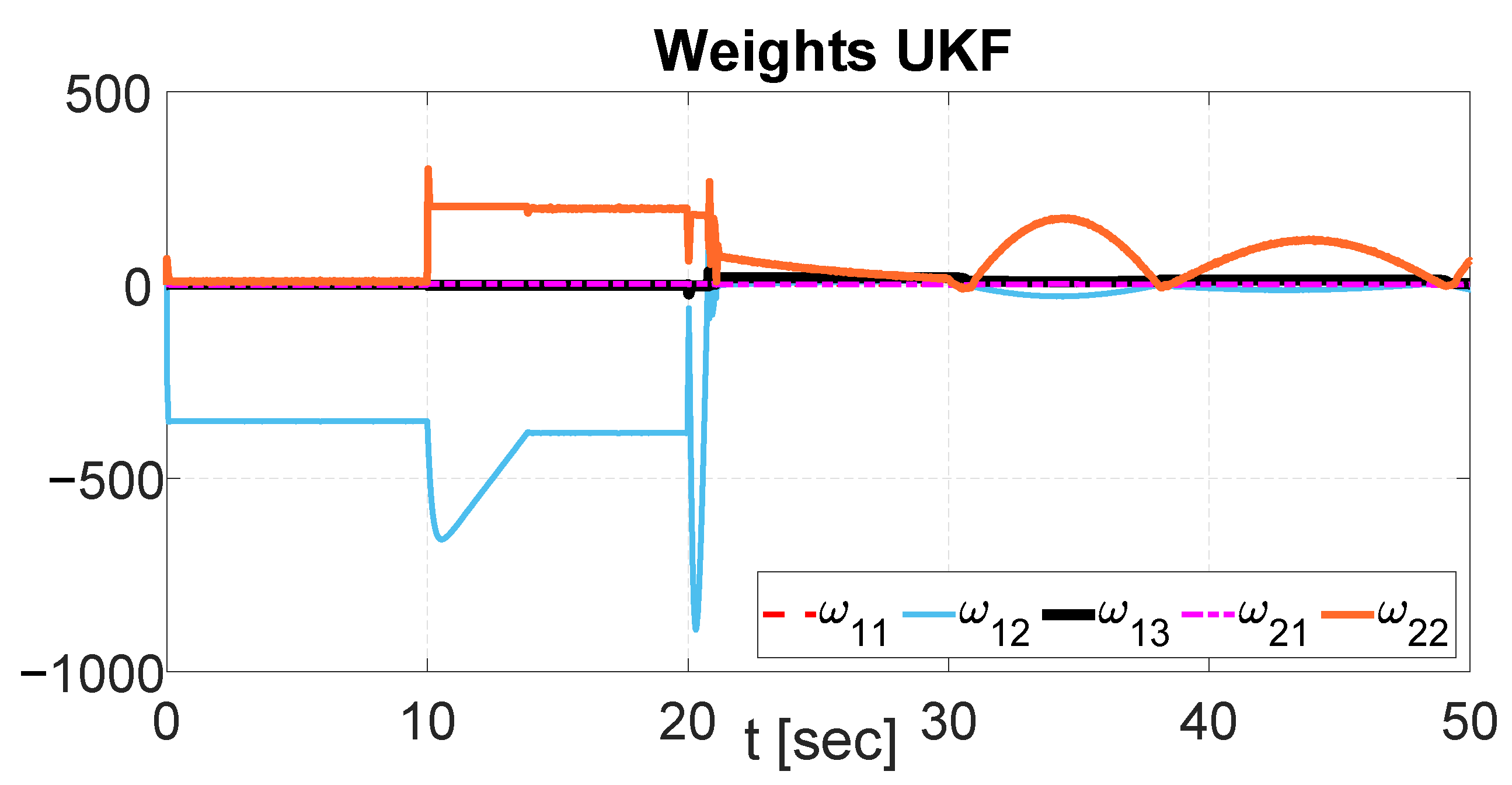
Figure 12.
Weight adjustment with UKF.
Figure 12.
Weight adjustment with UKF.
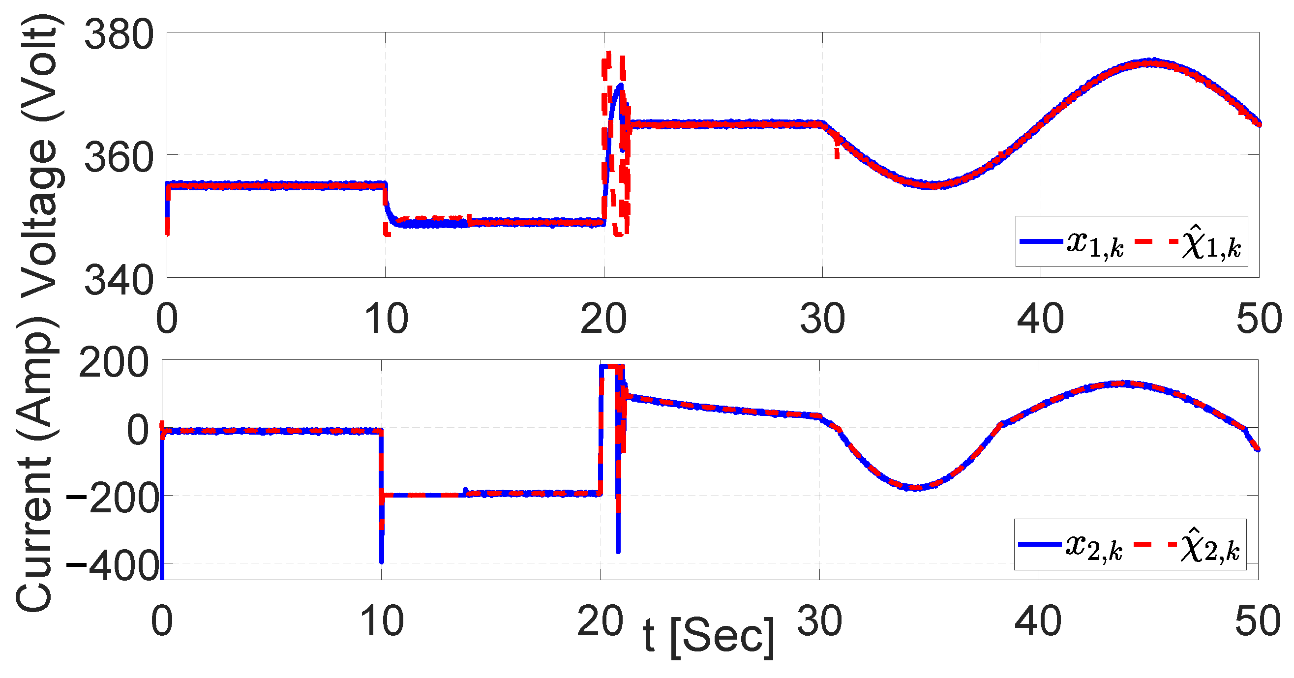
Figure 13.
System dynamics identification with UKF.
Figure 13.
System dynamics identification with UKF.
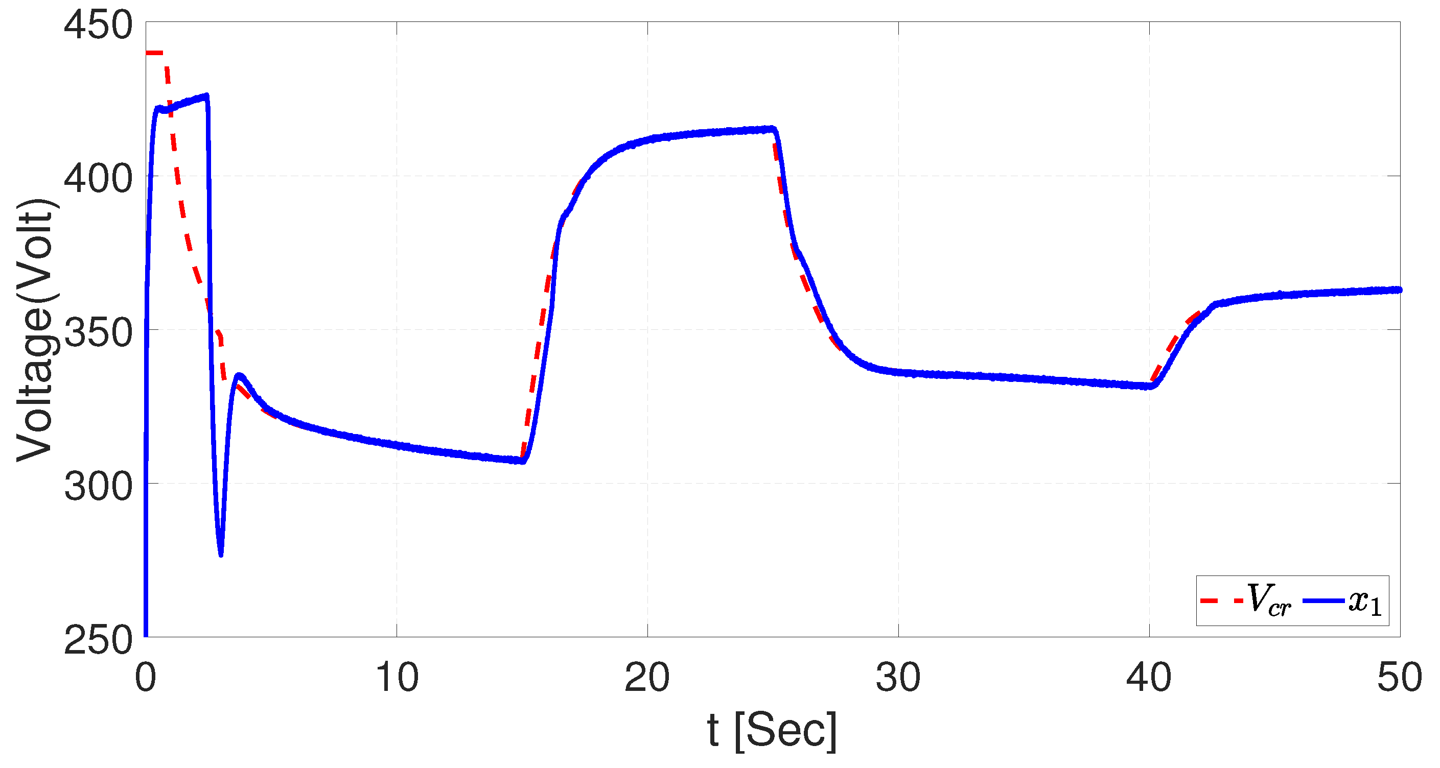
Figure 14.
Voltage dynamics trajectory tracking with EKF.
Figure 14.
Voltage dynamics trajectory tracking with EKF.
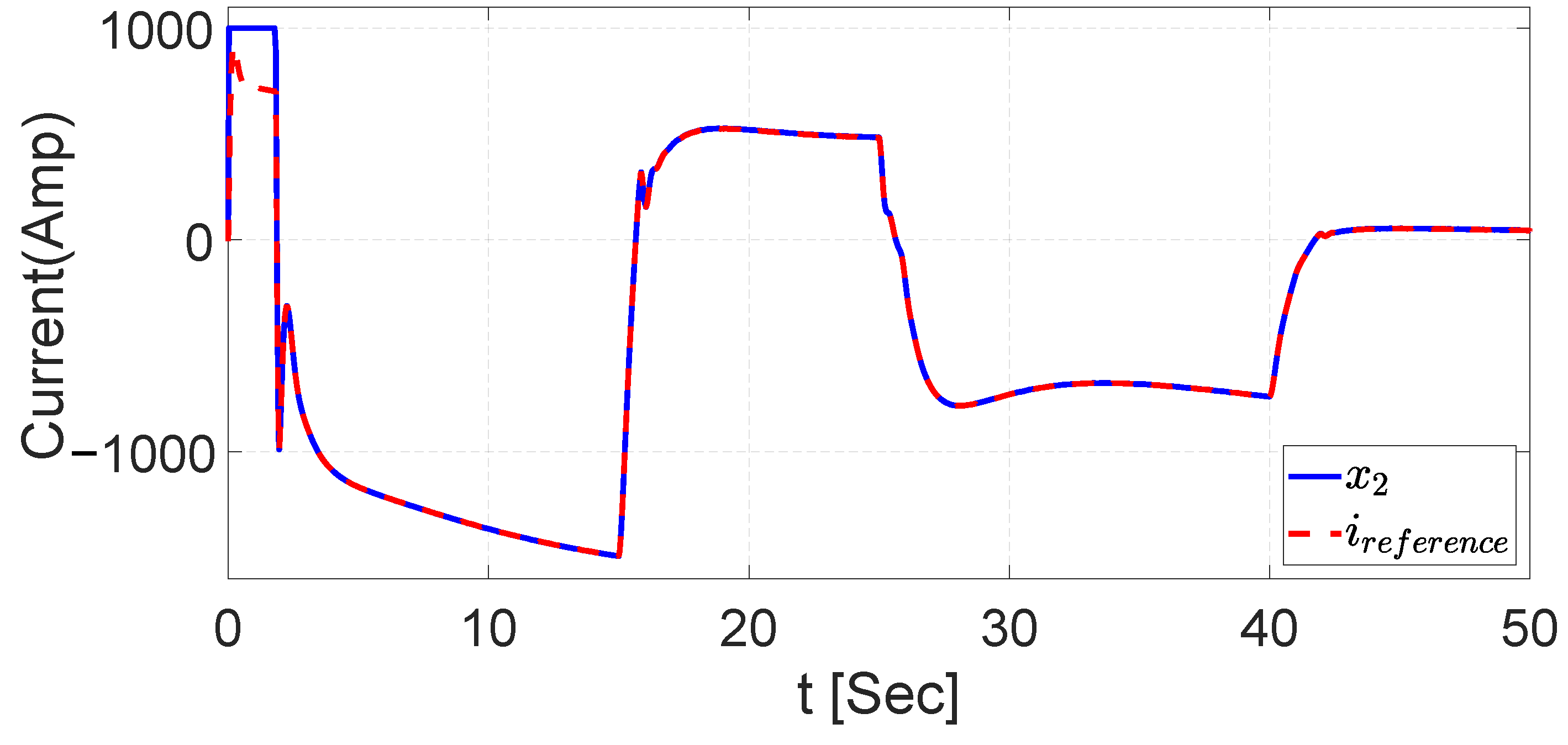
Figure 15.
Current dynamics trajectory tracking with EKF.
Figure 15.
Current dynamics trajectory tracking with EKF.
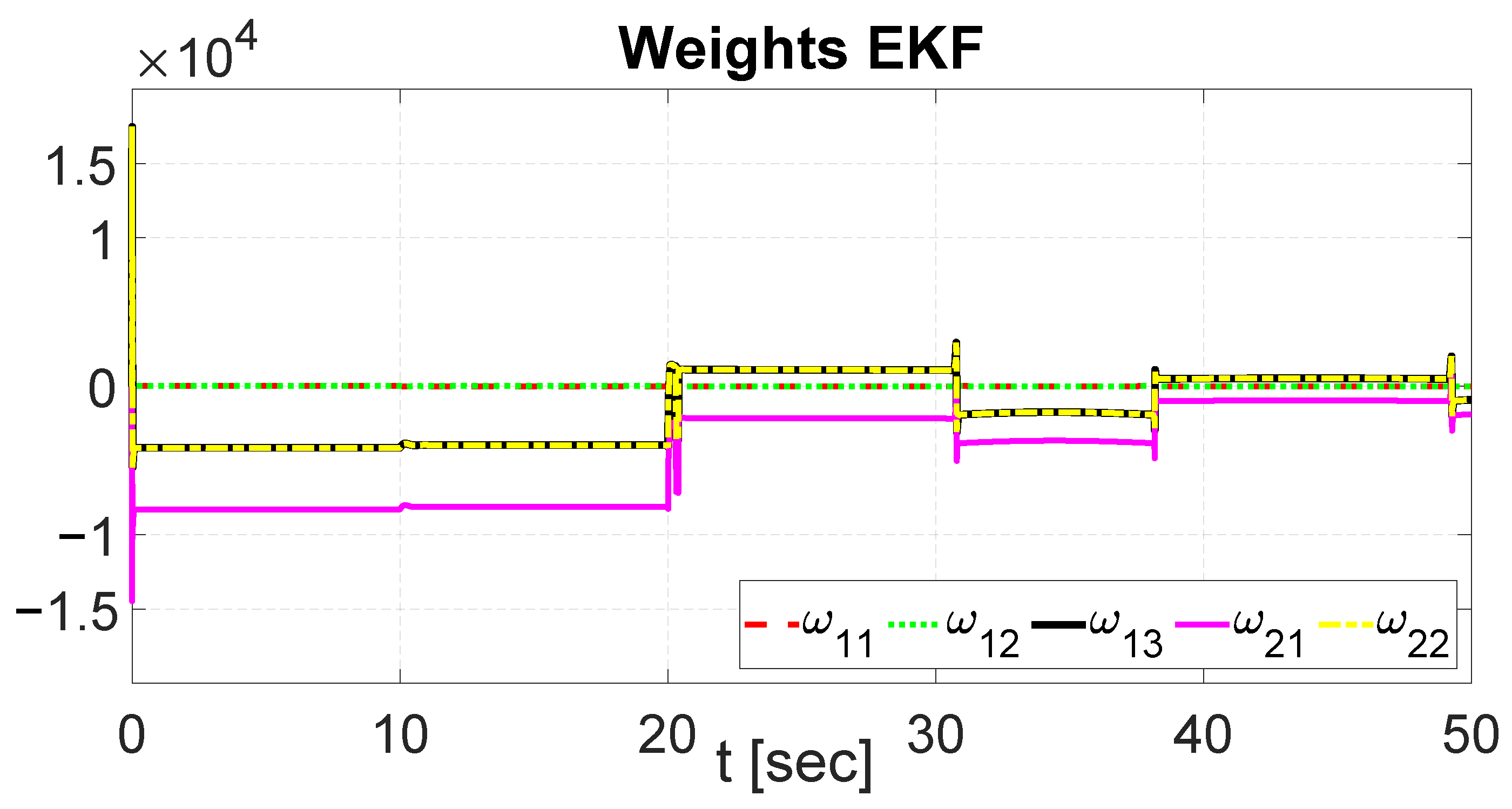
Figure 16.
Weight adjustment with EKF.
Figure 16.
Weight adjustment with EKF.
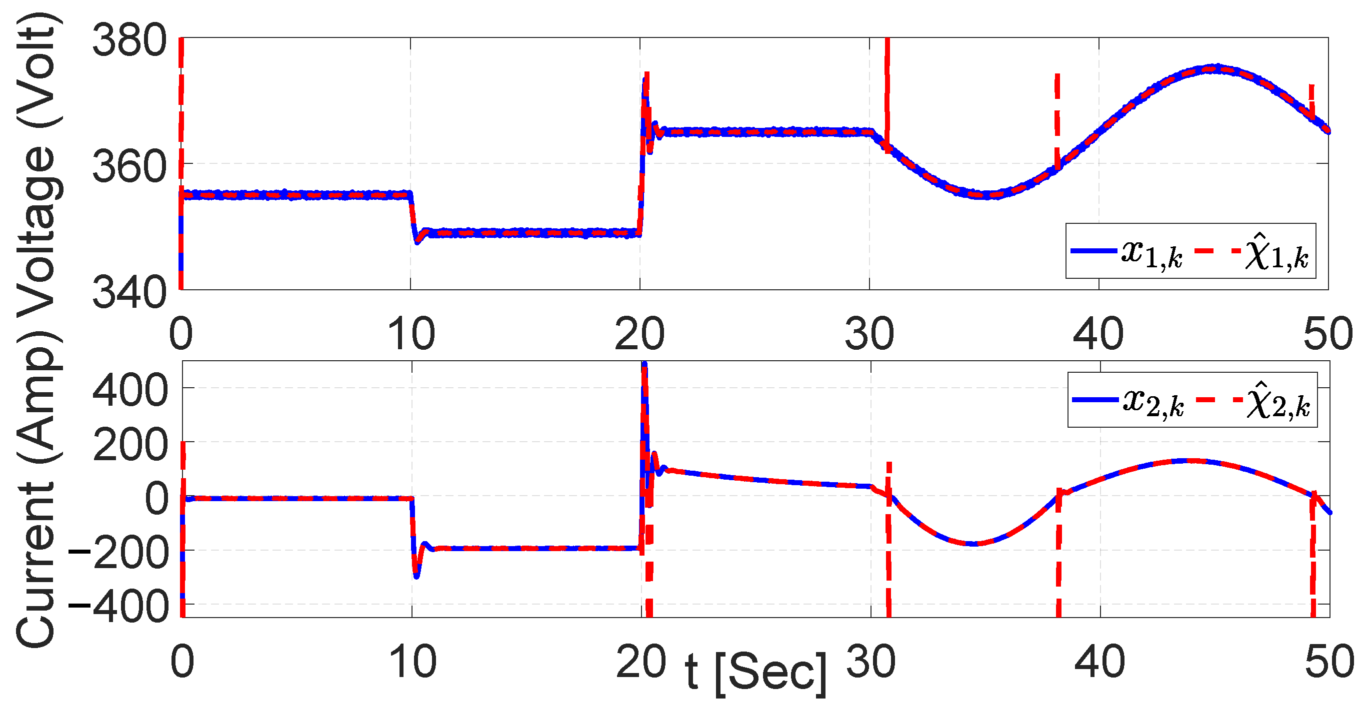
Figure 17.
System dynamics identification with EKF.
Figure 17.
System dynamics identification with EKF.
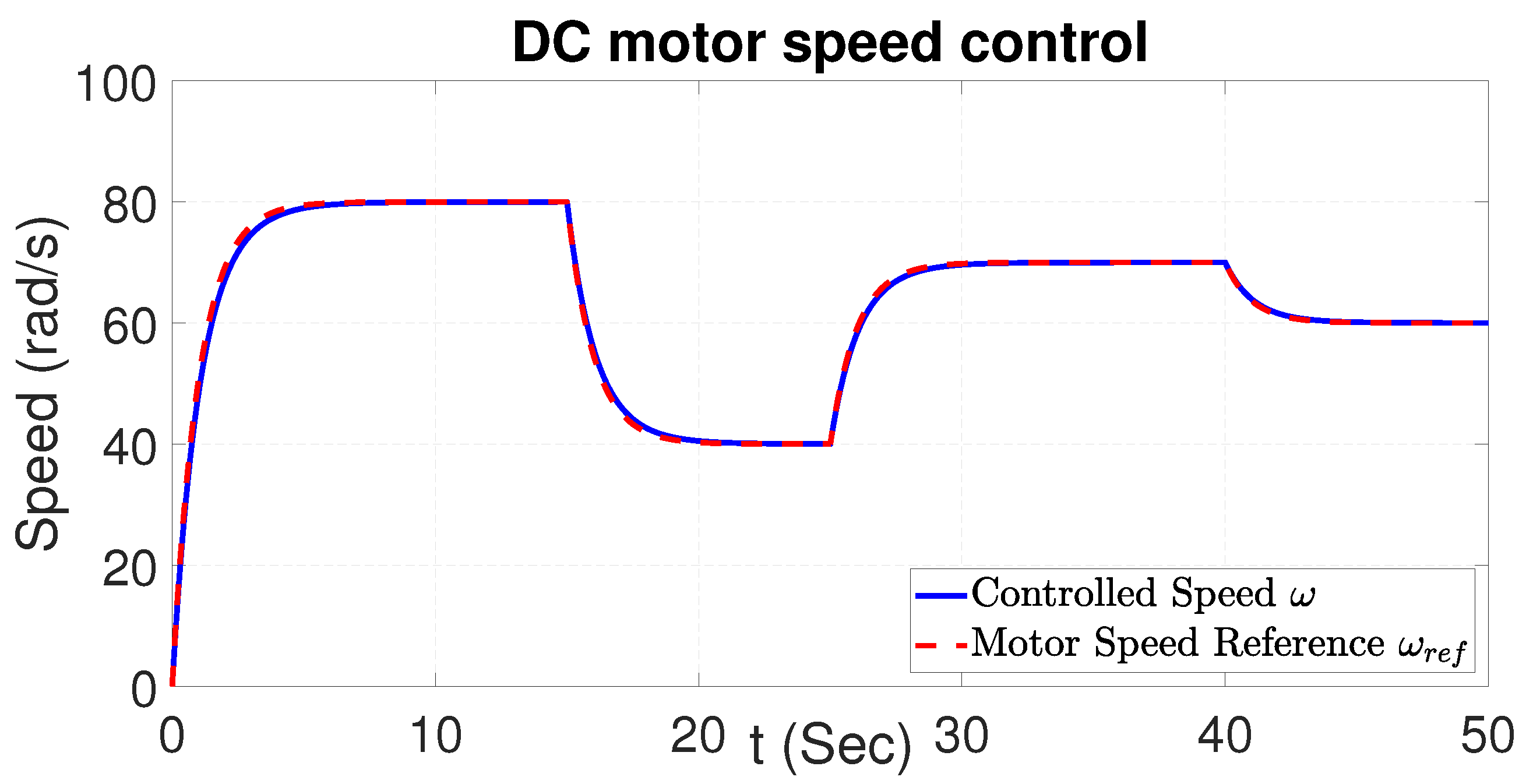
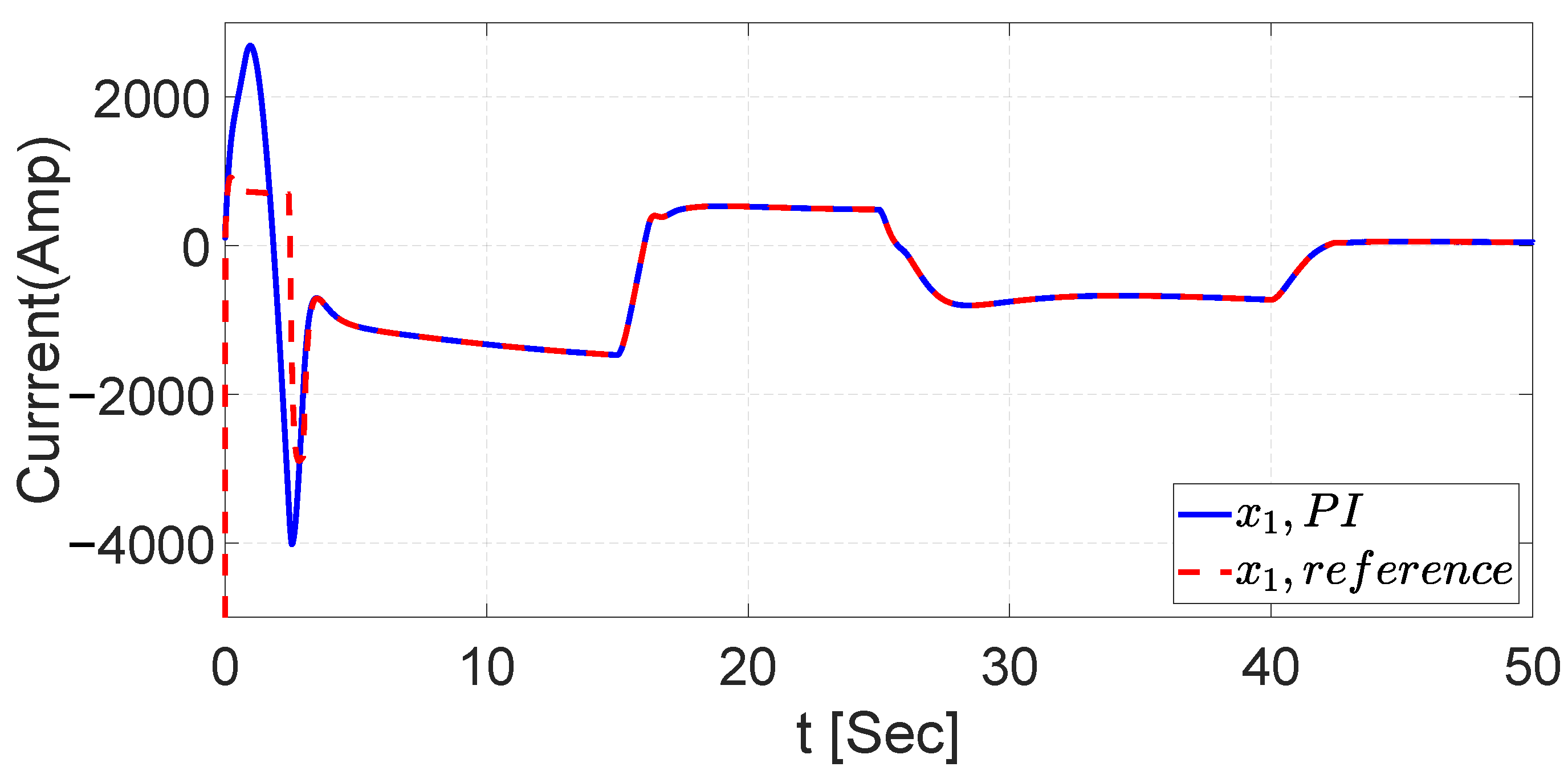
Figure 18.
Motor speed control with PI.
Figure 18.
Motor speed control with PI.
Figure 19.
AES voltage during regenerative braking with UKF.
Figure 19.
AES voltage during regenerative braking with UKF.
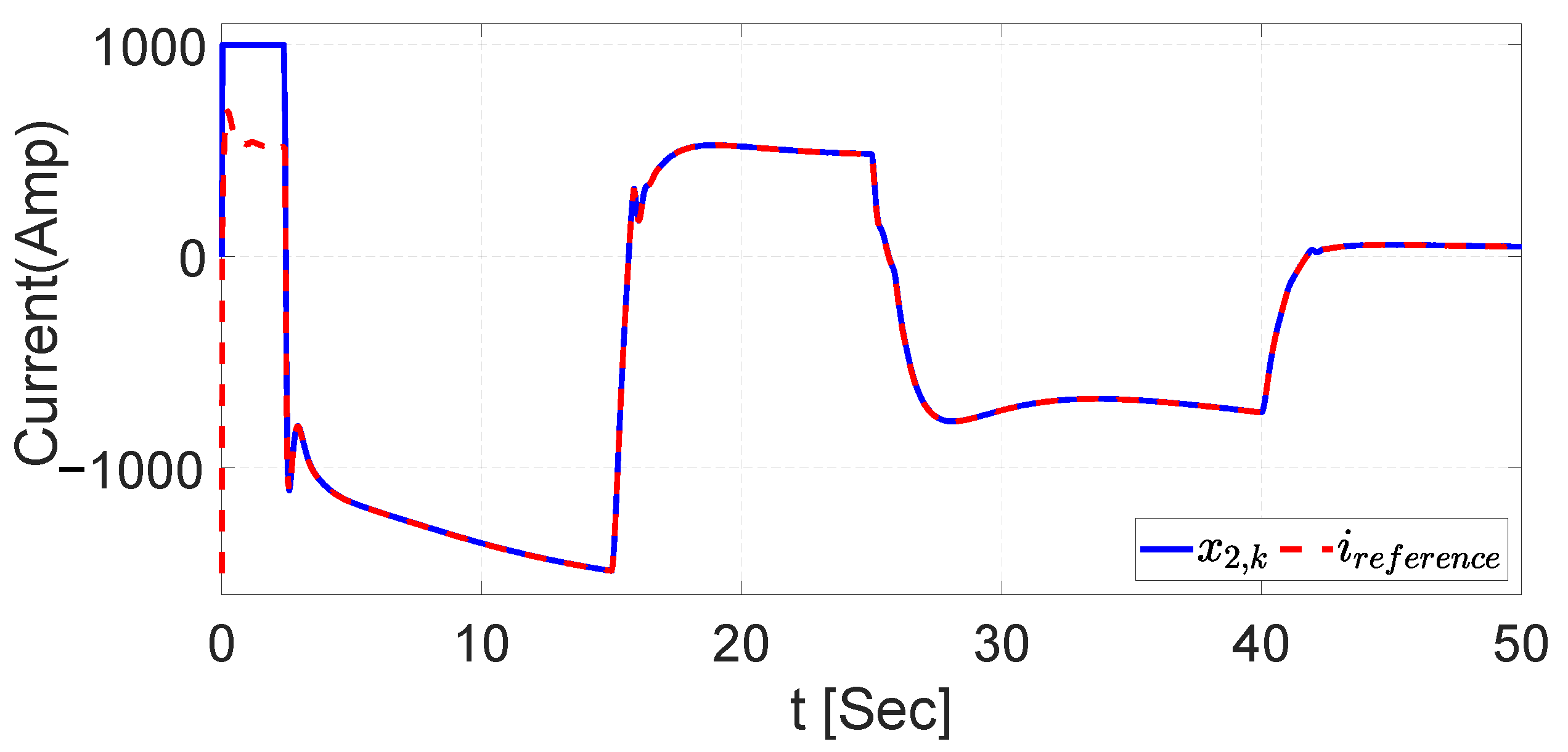
Figure 20.
AES current during regenerative braking with UKF.
Figure 20.
AES current during regenerative braking with UKF.
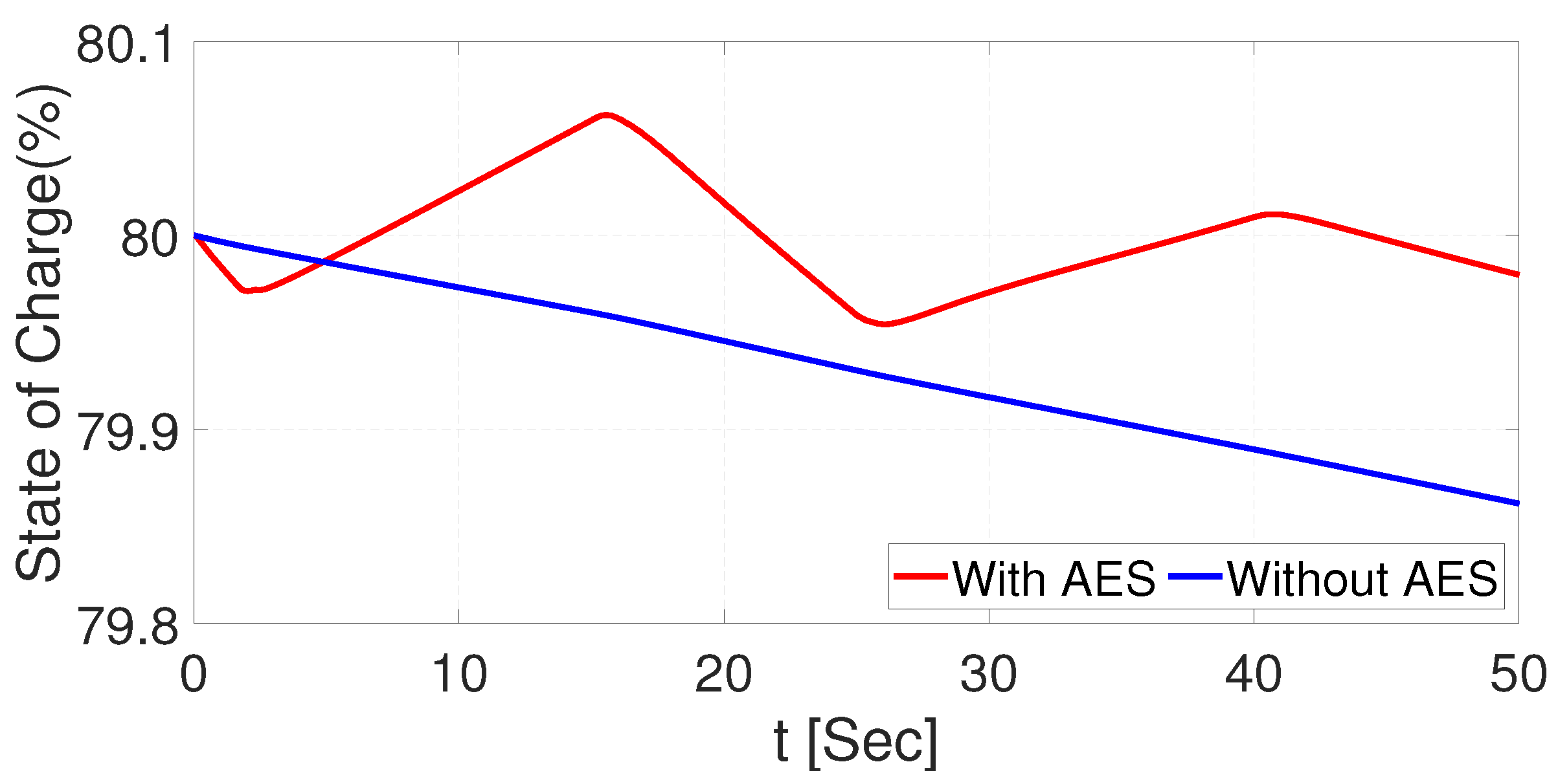
Figure 21.
SOC comparison of the battery with and without AES using UKF.
Figure 21.
SOC comparison of the battery with and without AES using UKF.
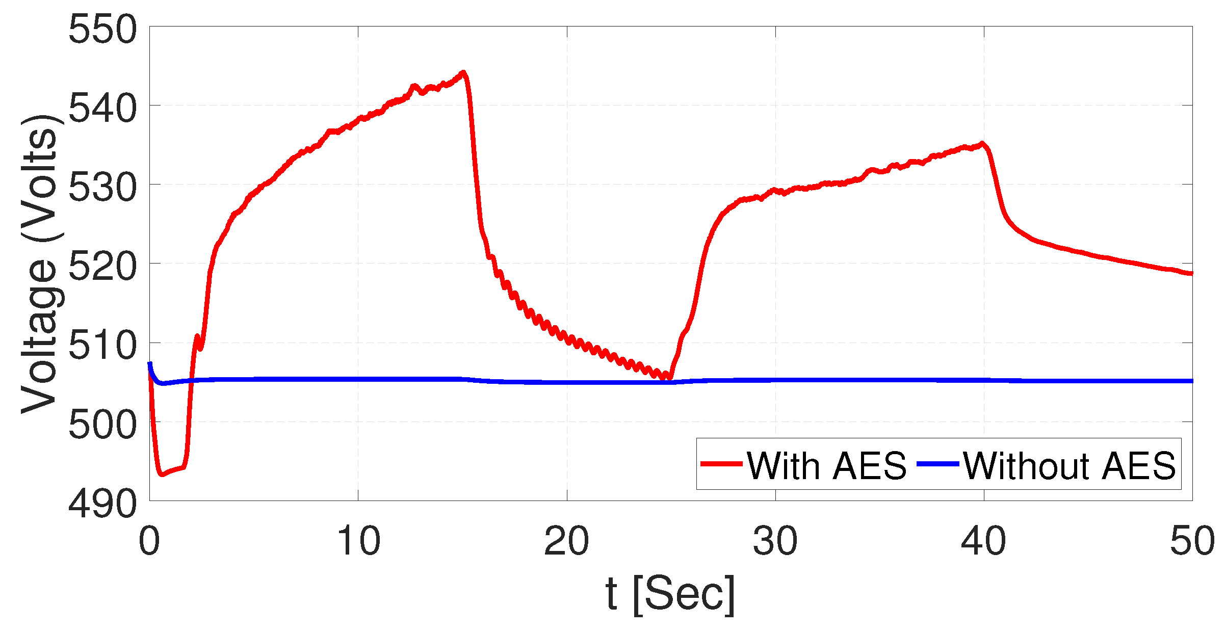
Figure 22.
Comparison of the battery bank voltage with and without AES using UKF.
Figure 22.
Comparison of the battery bank voltage with and without AES using UKF.
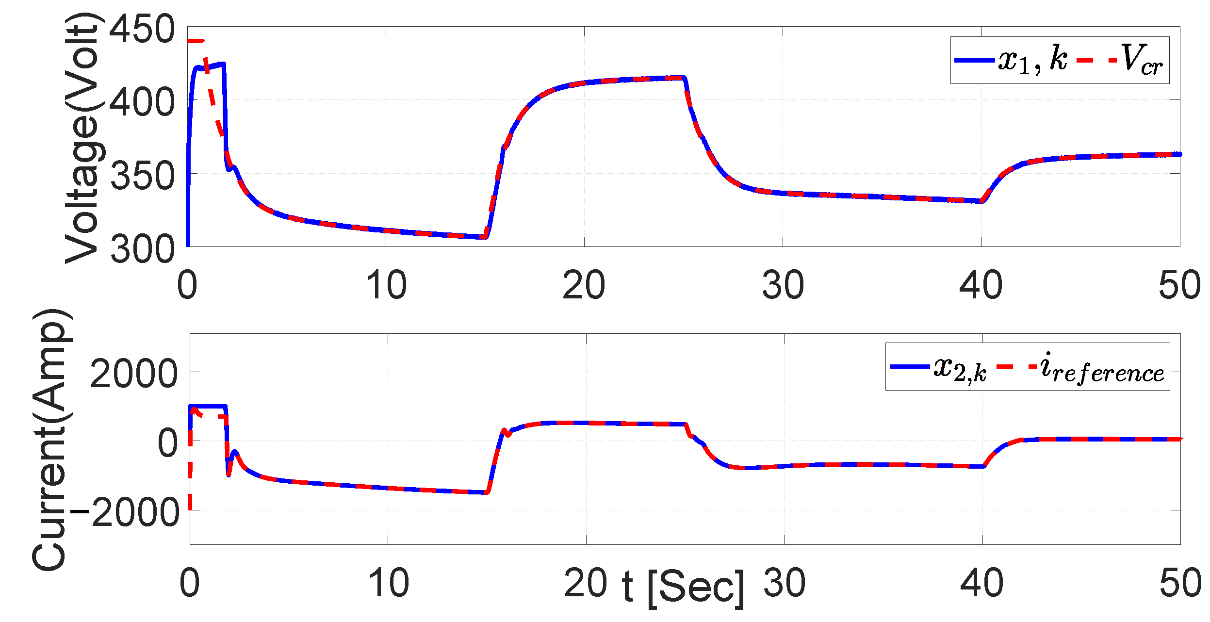
Figure 23.
AES voltage and current during regenerative braking using EKF.
Figure 23.
AES voltage and current during regenerative braking using EKF.
Figure 24.
MES battery bank SOC comparison with and without AES using EKF.
Figure 24.
MES battery bank SOC comparison with and without AES using EKF.
Figure 25.
MES battery bank voltage comparison with and without AES using EKF.
Figure 25.
MES battery bank voltage comparison with and without AES using EKF.
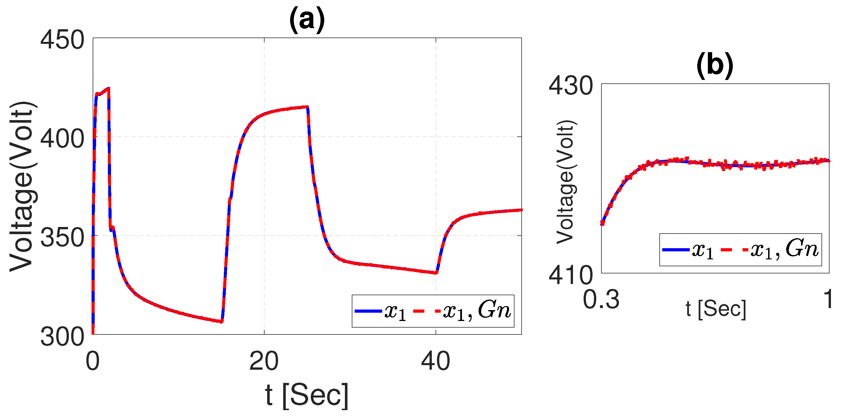
Figure 26.
(a) Voltage dynamics with Gaussian noise signal. (b) is a zoom of (a).
Figure 26.
(a) Voltage dynamics with Gaussian noise signal. (b) is a zoom of (a).
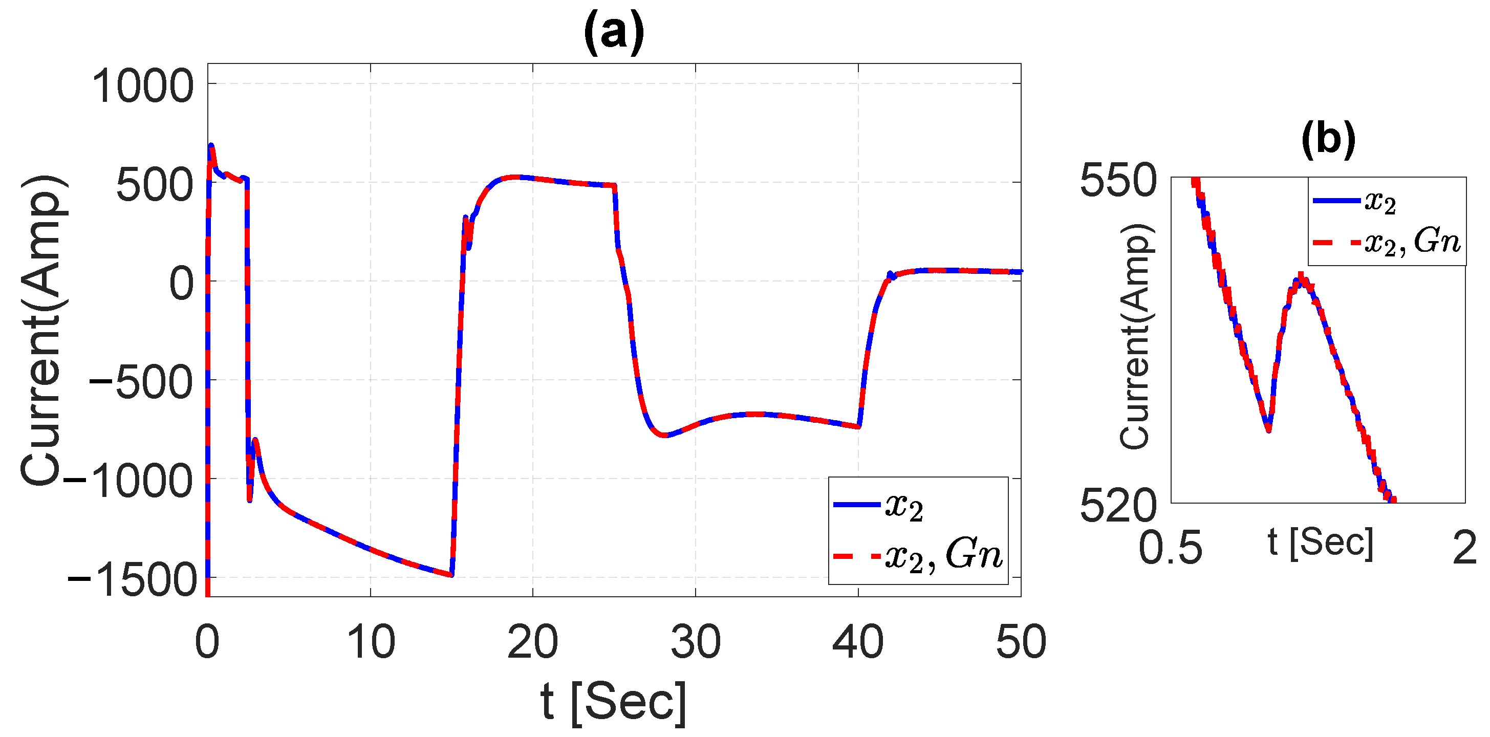
Figure 27.
(a) Current dynamics with Gaussian noise signal. (b) is a zoom of (a).
Figure 27.
(a) Current dynamics with Gaussian noise signal. (b) is a zoom of (a).
Figure 28.
Tracking trajectory with noise signal for voltage with UKF.
Figure 28.
Tracking trajectory with noise signal for voltage with UKF.
Figure 29.
Tracking trajectory with noise signal for current with UKF.
Figure 29.
Tracking trajectory with noise signal for current with UKF.
Figure 30.
(a) Voltage dynamics with Gaussian noise signal. (b) is a zoom of (a).
Figure 30.
(a) Voltage dynamics with Gaussian noise signal. (b) is a zoom of (a).
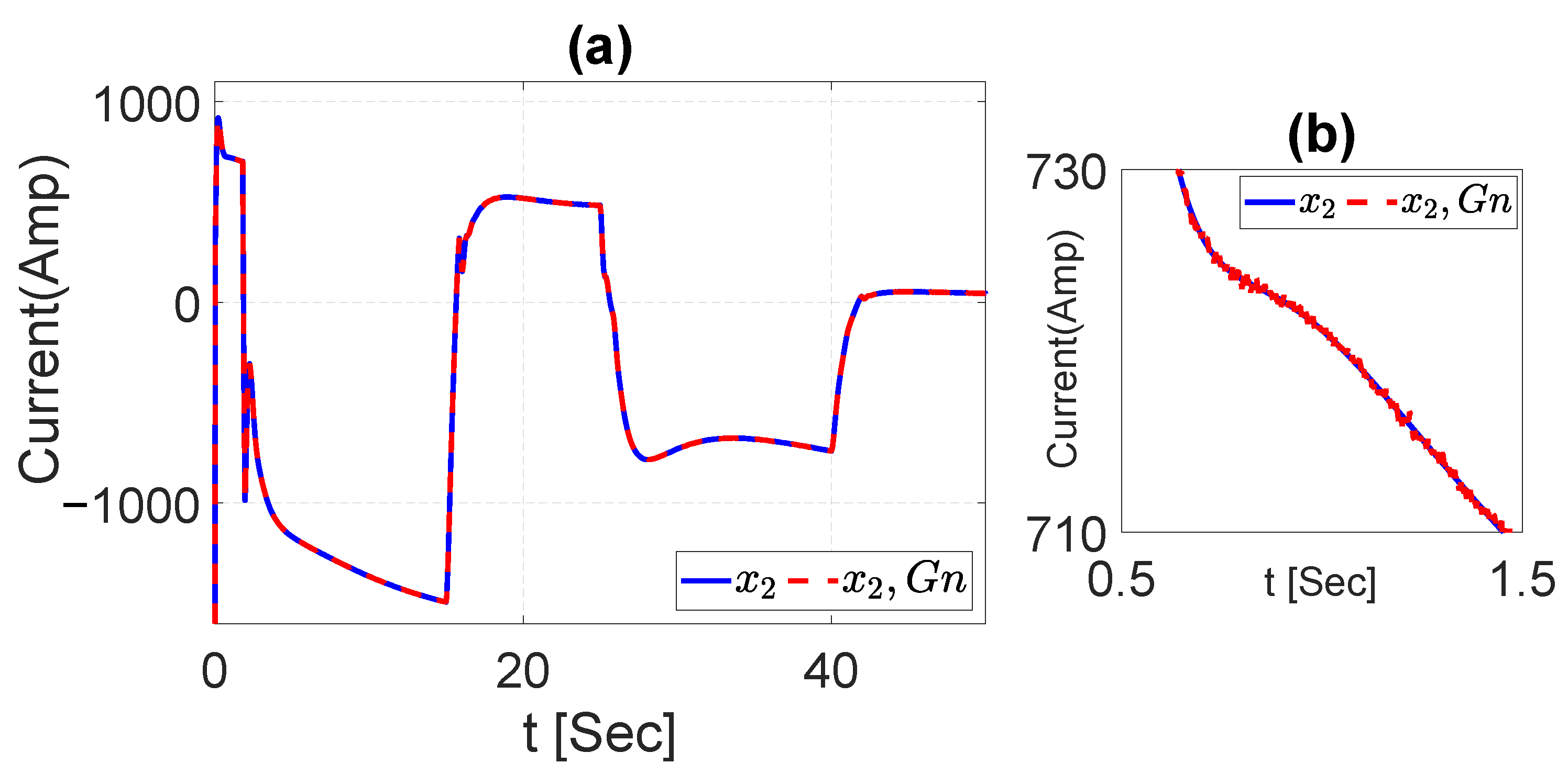
Figure 31.
(a) Current dynamics with Gaussian noise signal. (b) is a zoom of (a).
Figure 31.
(a) Current dynamics with Gaussian noise signal. (b) is a zoom of (a).
Figure 32.
Tracking trajectory with noise signal for voltage with EKF.
Figure 32.
Tracking trajectory with noise signal for voltage with EKF.
Figure 33.
Tracking trajectory with noise signal for current with EKF.
Figure 33.
Tracking trajectory with noise signal for current with EKF.
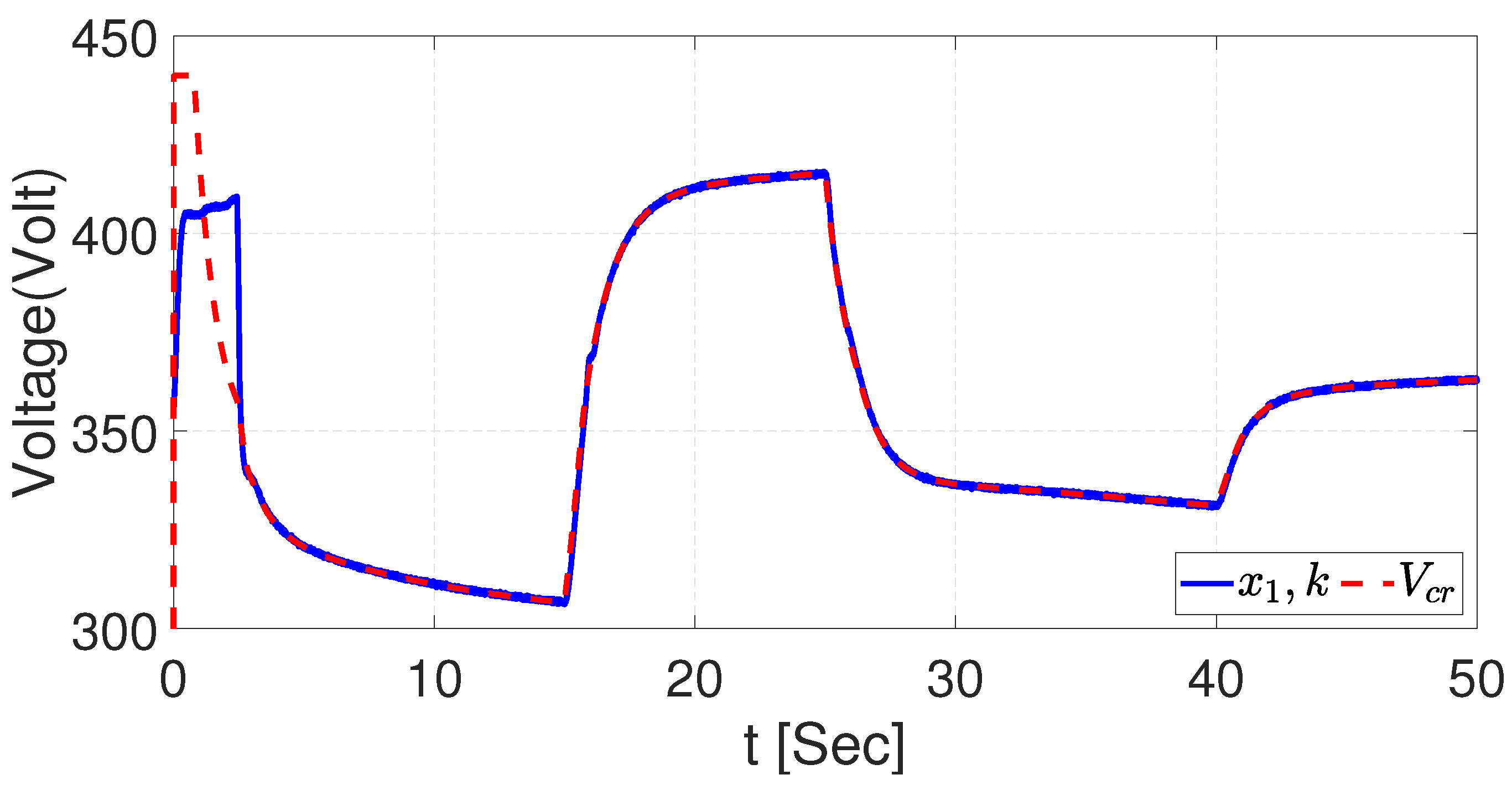
Figure 34.
Tracking trajectory with noise signal for voltage with PI.
Figure 34.
Tracking trajectory with noise signal for voltage with PI.
Figure 35.
Tracking trajectory with noise signal for current with PI.
Figure 35.
Tracking trajectory with noise signal for current with PI.
Figure 36.
Tracking trajectory with changes in the buck–boost converter for voltage with UKF.
Figure 36.
Tracking trajectory with changes in the buck–boost converter for voltage with UKF.
Figure 37.
Tracking trajectory with changes in the buck–boost converter for current with UKF.
Figure 37.
Tracking trajectory with changes in the buck–boost converter for current with UKF.
Figure 38.
Tracking trajectory with changes in the buck–boost converter for voltage with EKF.
Figure 38.
Tracking trajectory with changes in the buck–boost converter for voltage with EKF.
Figure 39.
Tracking trajectory with changes in the buck–boost converter for current with EKF.
Figure 39.
Tracking trajectory with changes in the buck–boost converter for current with EKF.
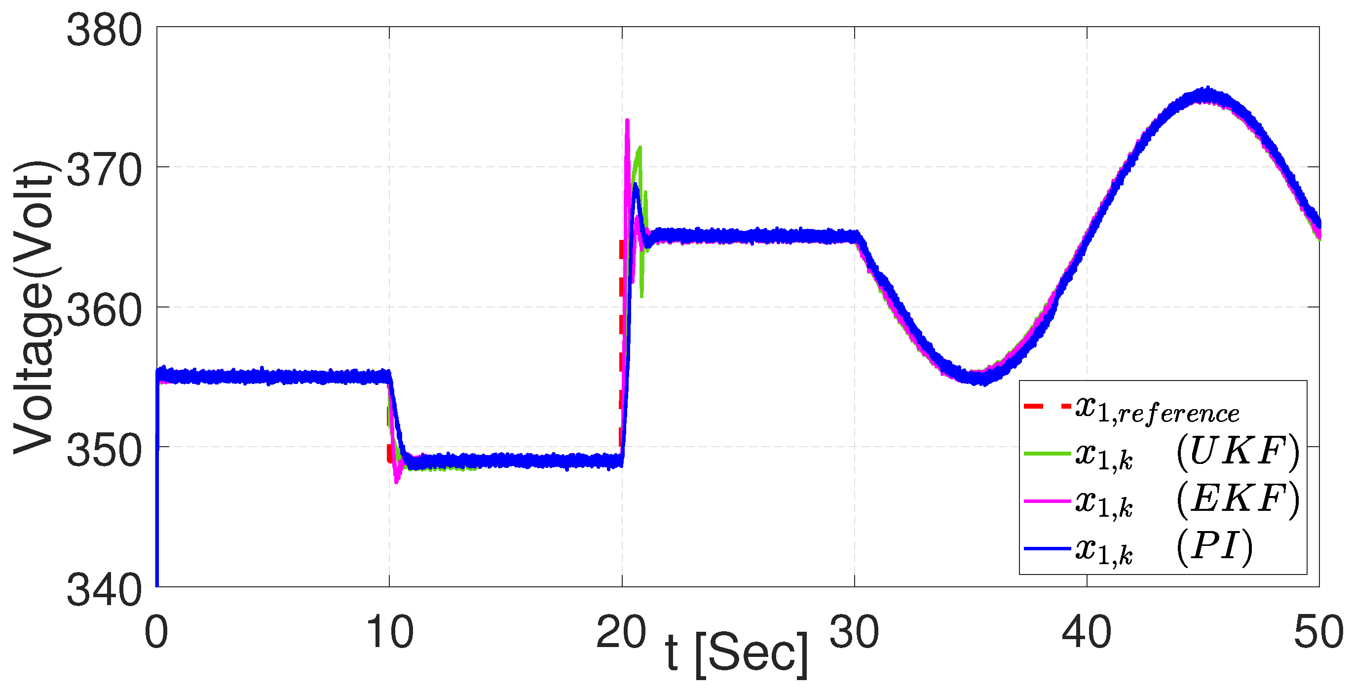
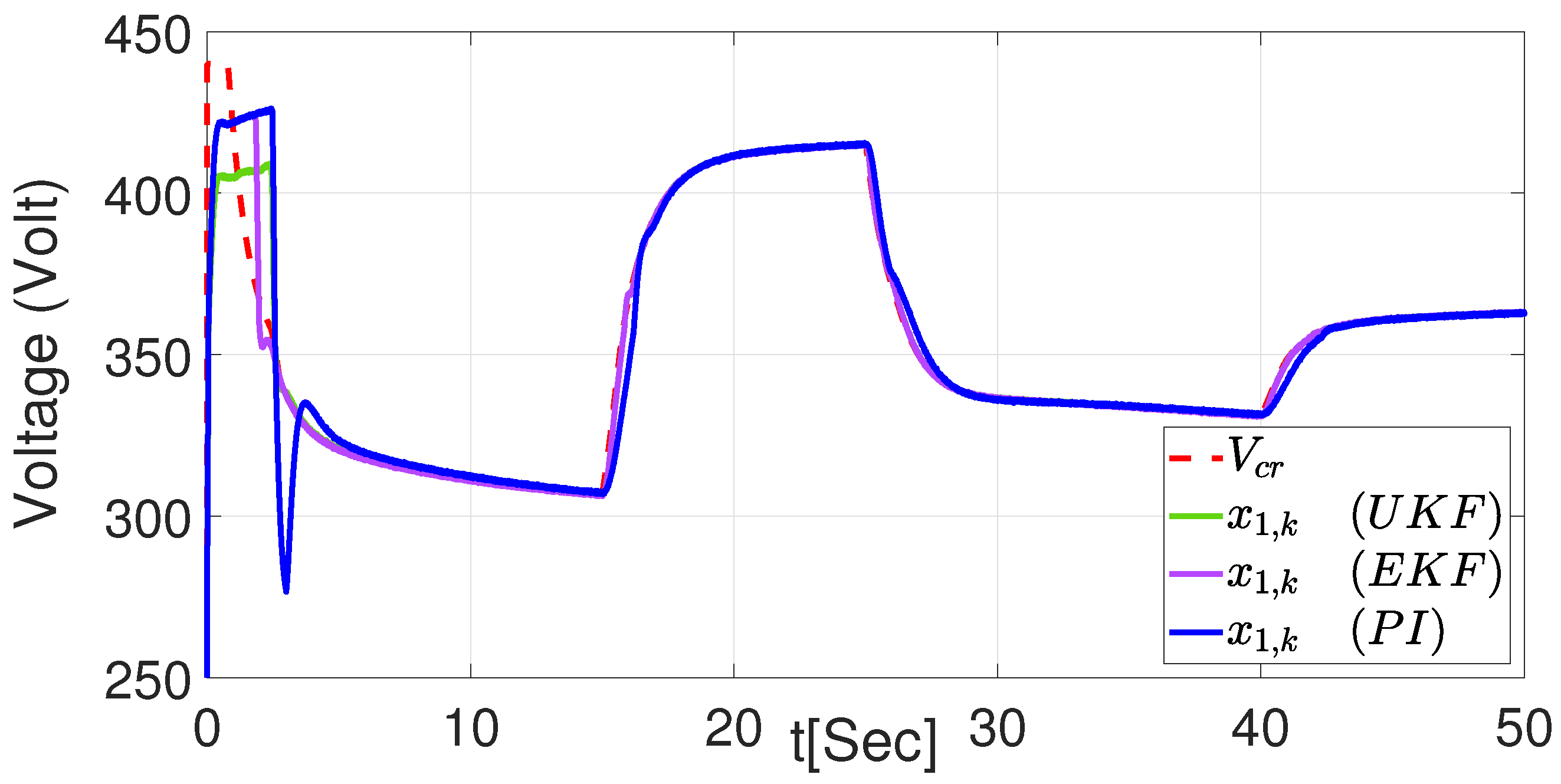
Figure 40.
Tracking trajectory with the three controllers for voltage .
Figure 40.
Tracking trajectory with the three controllers for voltage .
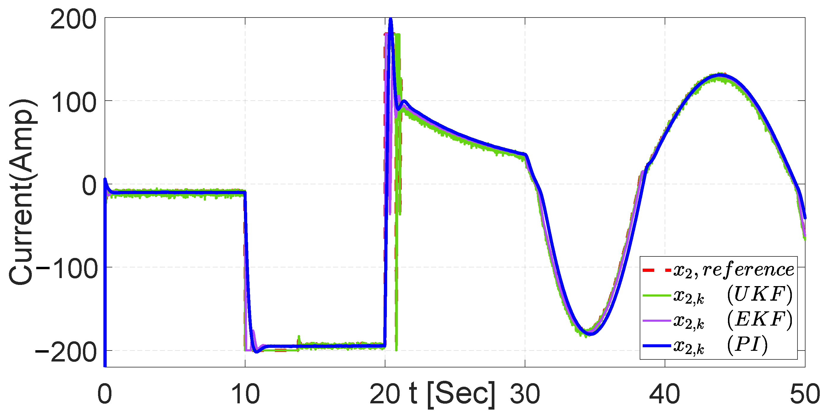
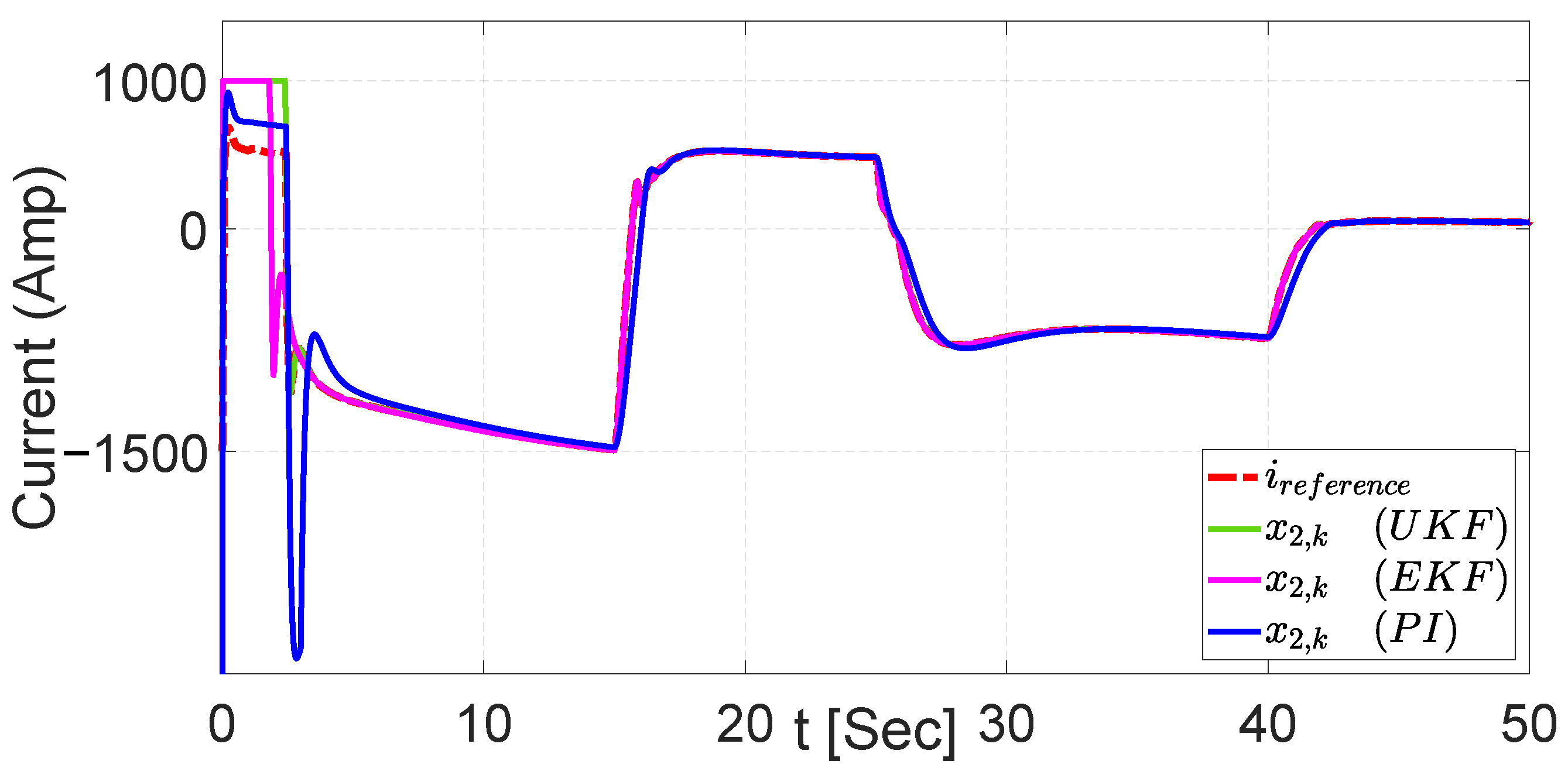
Figure 41.
Tracking trajectory with the three controllers for current .
Figure 41.
Tracking trajectory with the three controllers for current .
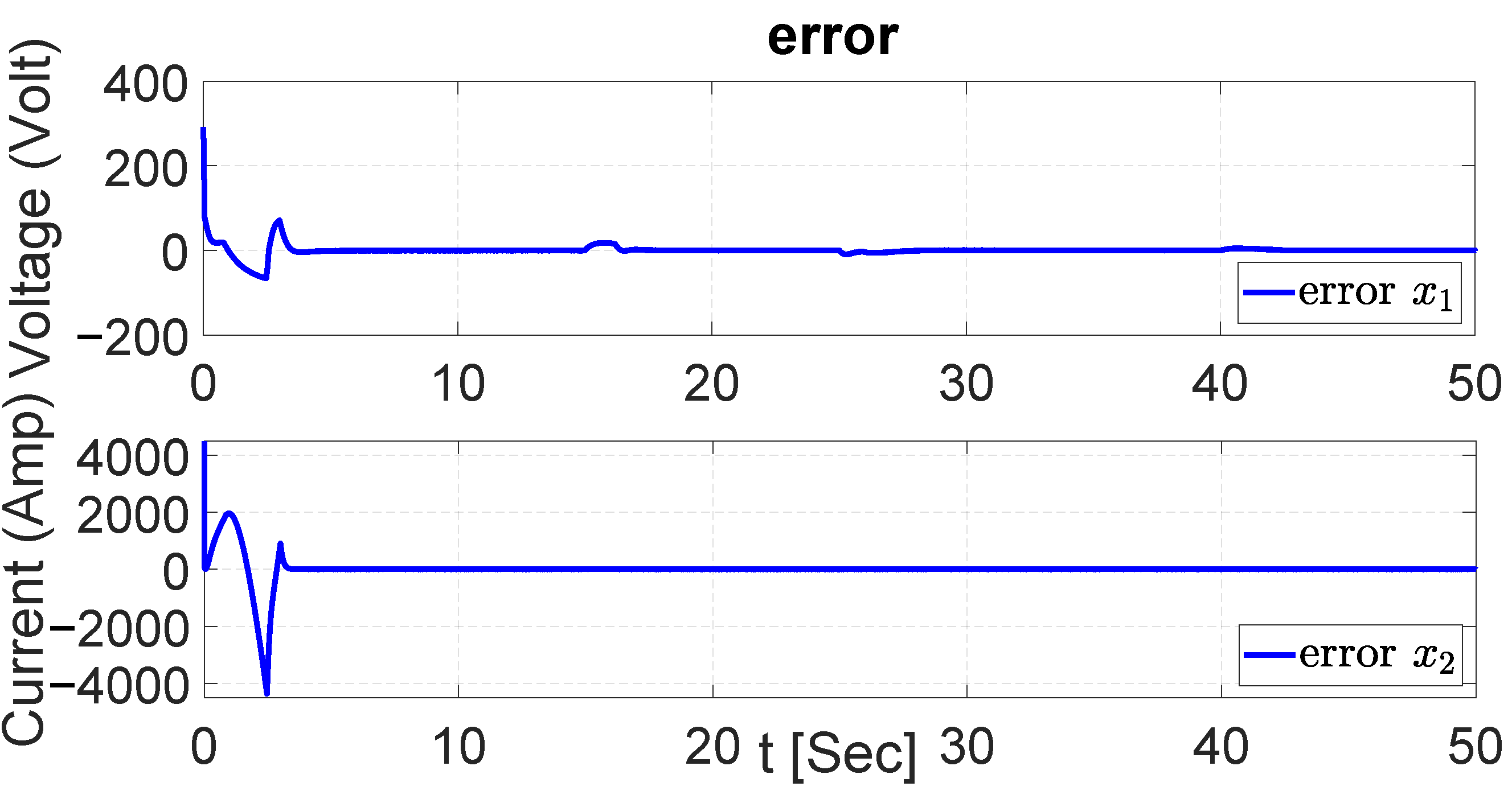
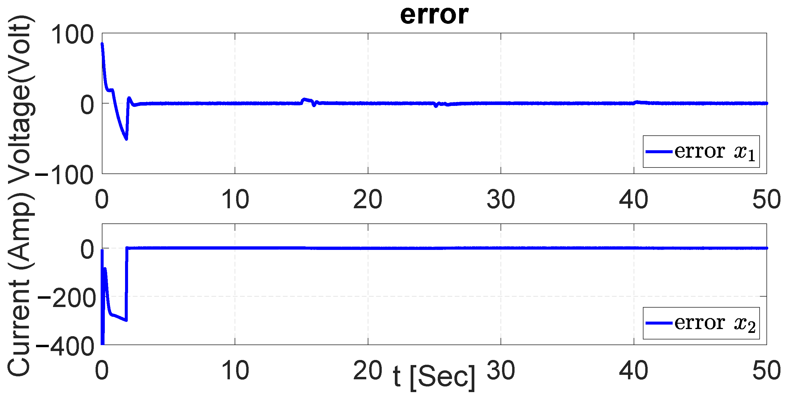
Figure 42.
Error in both dynamics with UKF.
Figure 42.
Error in both dynamics with UKF.
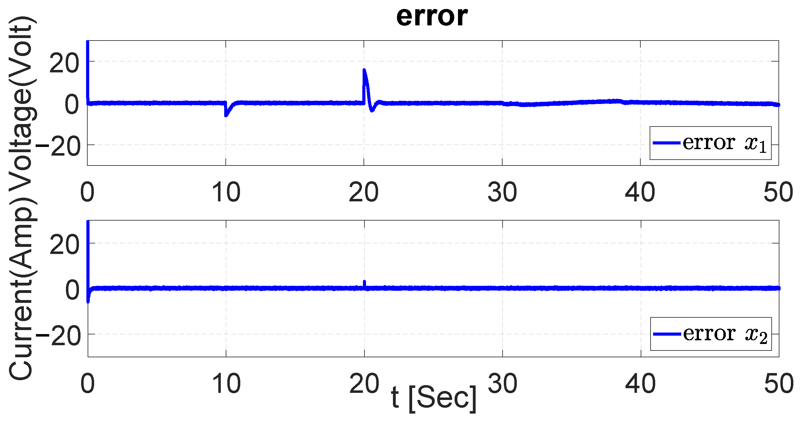
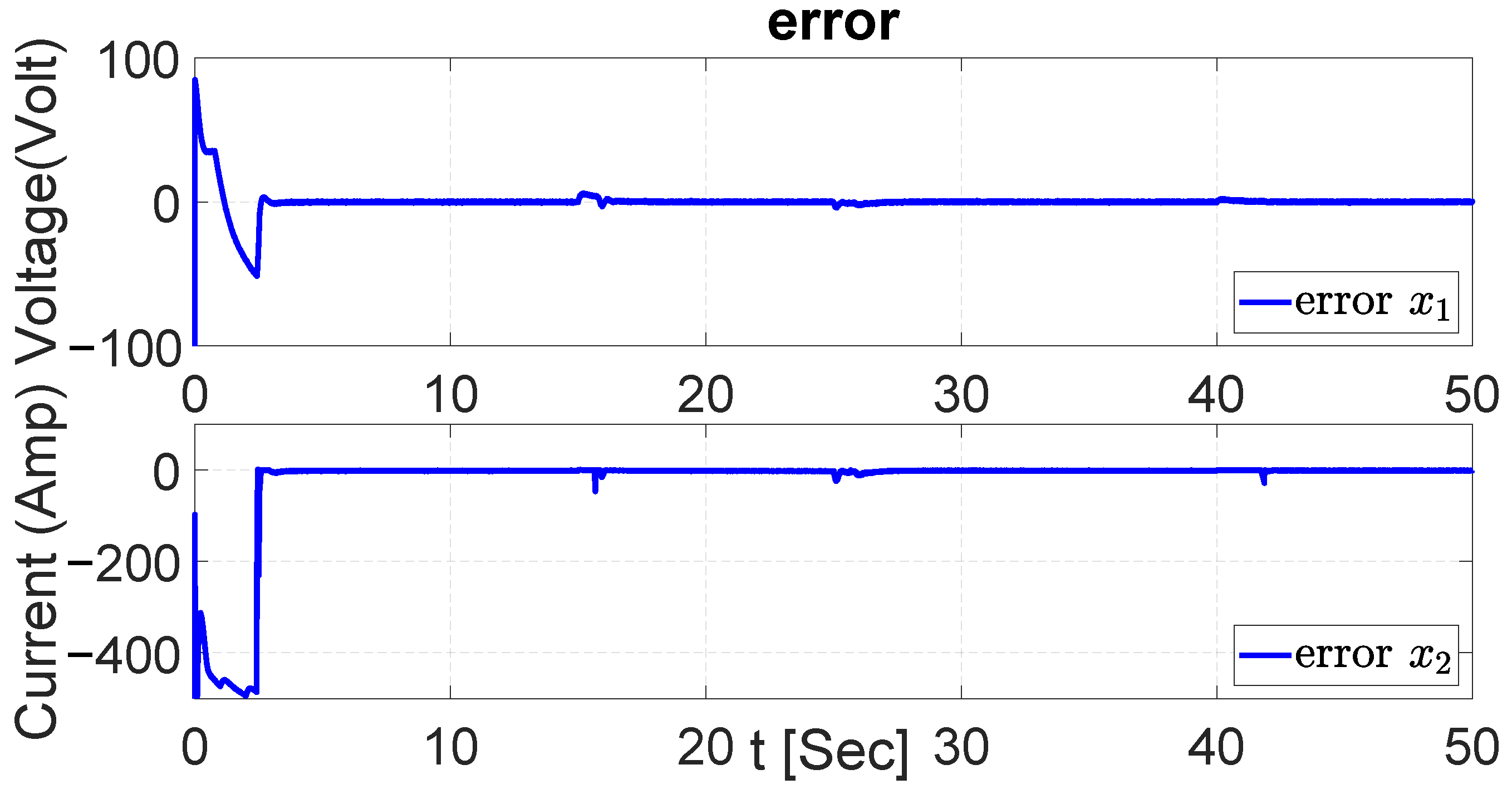
Figure 43.
Error in both dynamics with EKF.
Figure 43.
Error in both dynamics with EKF.
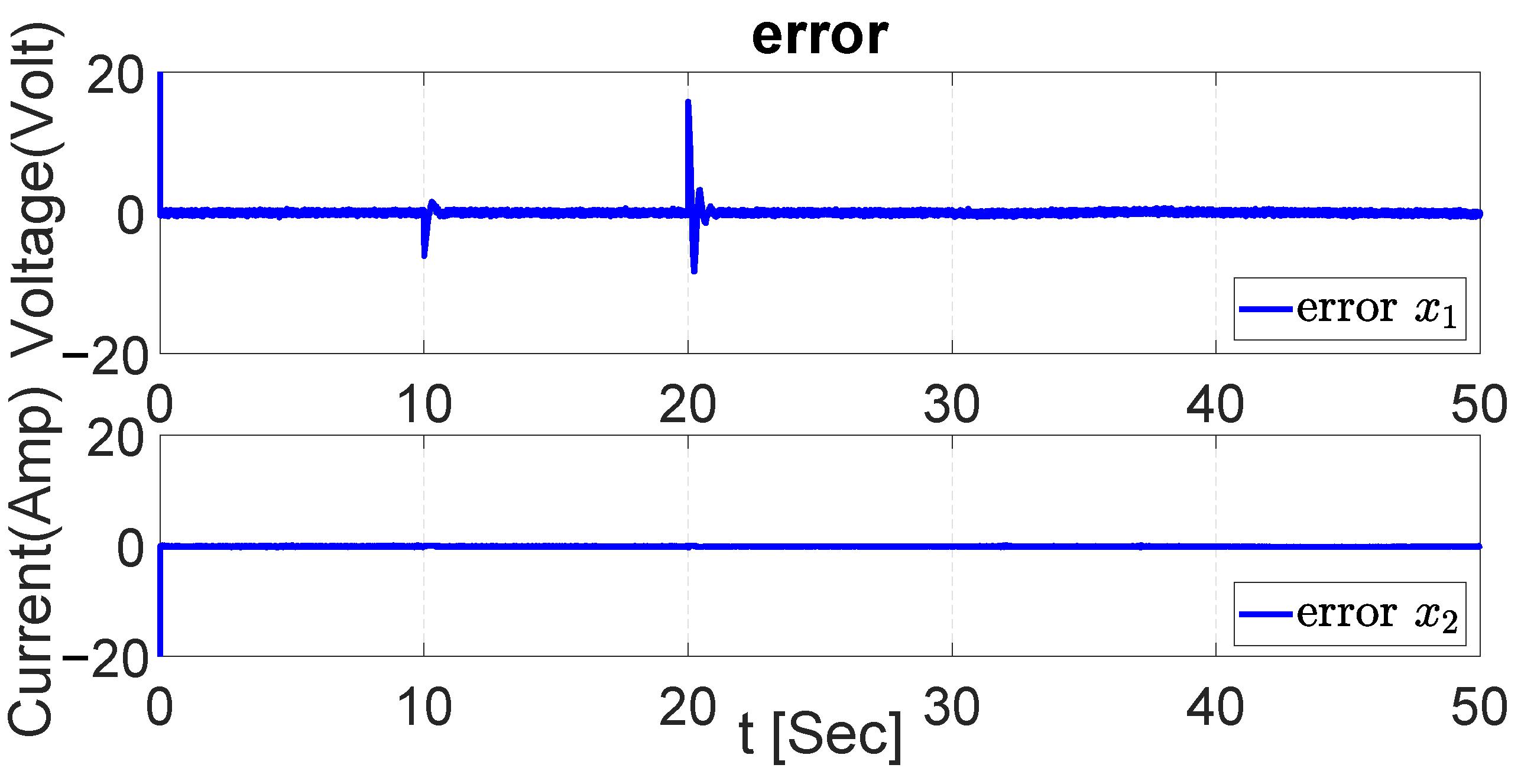
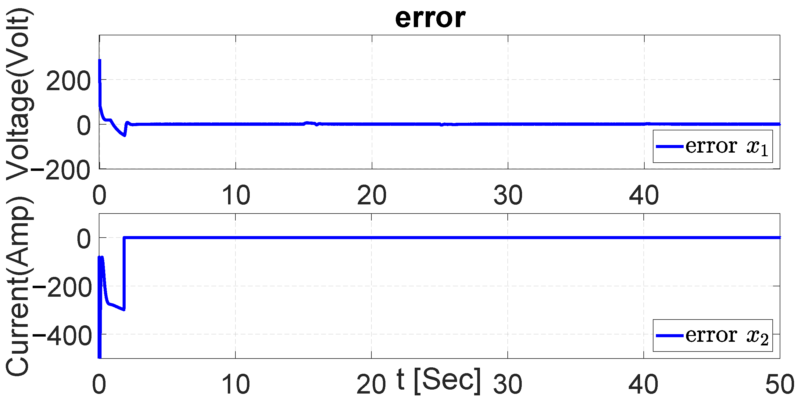
Figure 44.
Error in both dynamics with PI.
Figure 44.
Error in both dynamics with PI.
Figure 45.
Tracking trajectory with the three controllers for voltage with regenerative braking system.
Figure 45.
Tracking trajectory with the three controllers for voltage with regenerative braking system.
Figure 46.
Tracking trajectory with the three controllers for current with regenerative braking system.
Figure 46.
Tracking trajectory with the three controllers for current with regenerative braking system.
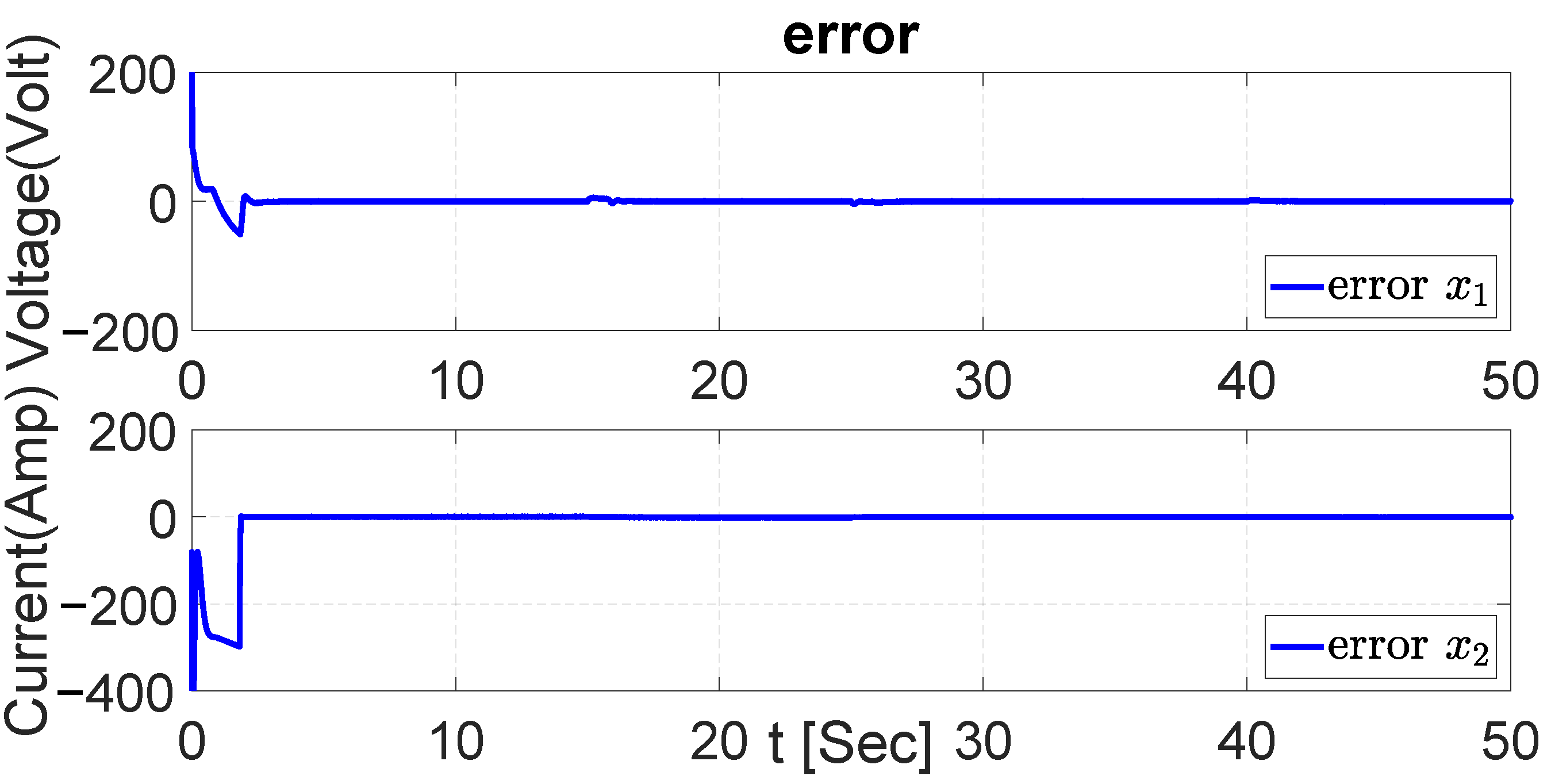
Figure 47.
Error in both dynamics during regenerative braking with UKF.
Figure 47.
Error in both dynamics during regenerative braking with UKF.
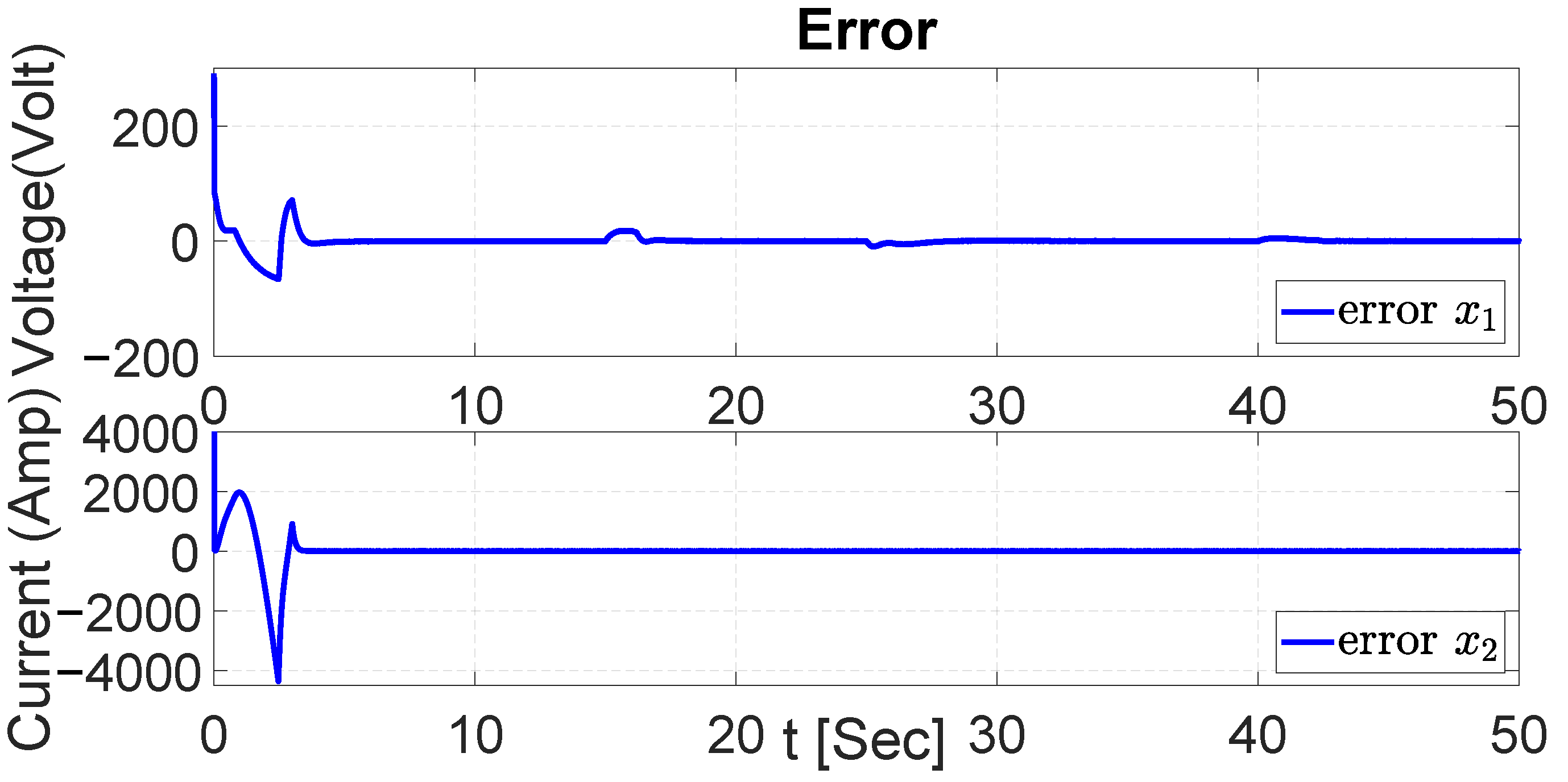
Figure 48.
Error in both dynamics during regenerative braking with EKF.
Figure 48.
Error in both dynamics during regenerative braking with EKF.
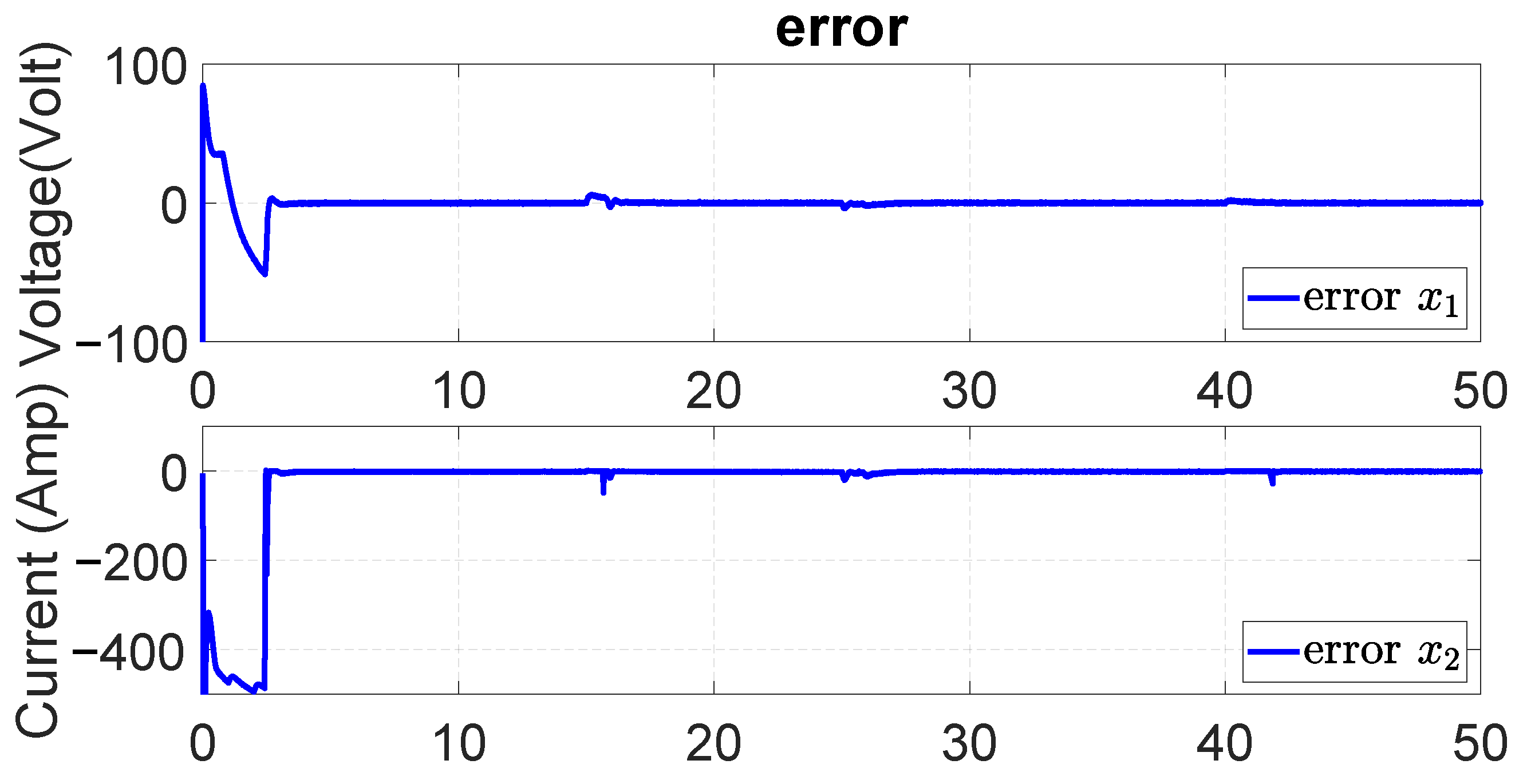
Figure 49.
Error in both dynamics during regenerative braking with PI.
Figure 49.
Error in both dynamics during regenerative braking with PI.
Figure 50.
Error in both dynamics with Gaussian noise with UKF.
Figure 50.
Error in both dynamics with Gaussian noise with UKF.
Figure 51.
Error in both dynamics with Gaussian noise with EKF.
Figure 51.
Error in both dynamics with Gaussian noise with EKF.
Figure 52.
Error in both dynamics with Gaussian noise with PI.
Figure 52.
Error in both dynamics with Gaussian noise with PI.
Figure 53.
Error in both dynamics with changes in buck–boost converter parameters with UKF.
Figure 53.
Error in both dynamics with changes in buck–boost converter parameters with UKF.
Figure 54.
Error in both dynamics with changes in buck–boost converter parameters with EKF.
Figure 54.
Error in both dynamics with changes in buck–boost converter parameters with EKF.
Figure 55.
Error in both dynamics with changes in buck–boost converter parameters with PI.
Figure 55.
Error in both dynamics with changes in buck–boost converter parameters with PI.
Table 1.
Differences between EKF and UKF training algorithms.
Table 1.
Differences between EKF and UKF training algorithms.
| Extended Kalman Filter (EKF) | Unscented Kalman Filter (UKF) |
|---|
| Design parameters |
Analytical Jacobian matrices
| Scaling parameters
|
| Initialization |
|
| Prediction |
| |
| Observation |
| |
| Update |
|
Table 2.
Parameters of the AES and MES.
Table 2.
Parameters of the AES and MES.
| Description | Unit |
|---|
| Buck–boost converter resistance R | |
| Buck–boost converter inductance L | 13 mH |
| Buck–boost converter capacitance | 2 mF |
| Buck–boost converter capacitance | 1 F |
| Supercapacitor voltage | 350 V |
| Battery bank voltage | 500 V |
| Initial SOC | 80% |
| Sampling time | 0.1 seg |
Table 3.
Chirp signal parameters.
Table 3.
Chirp signal parameters.
| Chirp Signals Parameters |
|---|
|
Controller
|
Initial Frequency
|
Target Time (s)
|
Frequency at Target Time (Hz)
|
|---|
| Chirp signal for voltage | 0.5 Hz | 25 | 0.6 Hz |
| Chirp signal for current | 0.5 Hz | 10 | 0.5 Hz |
Table 4.
Parameters of the DC motor.
Table 4.
Parameters of the DC motor.
| Description | Unit |
|---|
| Armature resistance | |
| Armature inductance | H |
| Field resistance | |
| Field inductance | 156 H |
| Field-armature mutual inductance | H |
| Power | 5 Hp |
| DC voltage | 240 v |
| Rated speed rpm | 1750 rpm |
| Field voltage | 300 v |
Table 5.
Parameters of the AES and MES with changes for the robustness test.
Table 5.
Parameters of the AES and MES with changes for the robustness test.
| Description | Unit |
|---|
| Buck–boost converter resistance R | |
| Buck–boost converter inductance L | 13 mH |
| Buck–boost converter capacitance | 14 mF |
| Buck–boost converter capacitance | 6 F |
| Supercapacitor voltage | 350 V |
| Battery bank voltage | 500 V |
| Initial SOC | 80% |
| Sampling time | seg |
Table 6.
MSE and EES in without regenerative braking system.
Table 6.
MSE and EES in without regenerative braking system.
| MSE and EES of Tracking Trajectories in |
|---|
|
Controller
|
MSE Value
|
EES Value
|
|---|
| NSMC with UKF | 72.9529 | |
| NSMC with EKF | 1.0585 | |
| PI | 1.7403 | |
Table 7.
MSE and EES in without regenerative braking system.
Table 7.
MSE and EES in without regenerative braking system.
| MSE and EES of Tracking Trajectories in |
|---|
|
Controller
|
MSE Value
|
EES Value
|
|---|
| NSMC with UKF | | |
| NSMC with EKF | 0.1362 | |
| PI | 270.1132 | |
Table 8.
MSE and EES in with regenerative braking system.
Table 8.
MSE and EES in with regenerative braking system.
| MSE and EES of Tracking Trajectories in |
|---|
|
Controller
|
MSE Value
|
EES Value
|
|---|
| NSMC with UKF | 45.2714 | |
| NSMC with EKF | 1.0321 | |
| PI | 132.4538 | |
Table 9.
MSE and EES in with regenerative braking system.
Table 9.
MSE and EES in with regenerative braking system.
| MSE and EES of Tracking Trajectories in |
|---|
|
Controller
|
MSE Value
|
EES Value
|
|---|
| NSMC with UKF | 1.9679 | |
| NSMC with EKF | 8.9223 | |
| PI | | |
Table 10.
MSE and EES in with Gaussian noise.
Table 10.
MSE and EES in with Gaussian noise.
| MSE and EES of Tracking Trajectories with Gaussian noise in |
|---|
|
Controller
|
MSE Value
|
EES Value
|
|---|
| NSMC with UKF | 73.4682 | |
| NSMC with EKF | 45.7588 | |
| PI | | |
Table 11.
MSE and EES in with Gaussian noise.
Table 11.
MSE and EES in with Gaussian noise.
| MSE and EES of Tracking Trajectories with Gaussian noise in |
|---|
|
Controller
|
MSE Value
|
EES Value
|
|---|
| NSMC with UKF | | |
| NSMC with EKF | | |
| PI | | |
Table 12.
MSE and EES in with changes in buck–boost converter parameters.
Table 12.
MSE and EES in with changes in buck–boost converter parameters.
| MSE and EES with Changes in Buck–Boost Converter Parameters in |
|---|
|
Controller
|
MSE Value
|
EES Value
|
|---|
| NSMC with UKF | | |
| NSMC with EKF | | |
| PI | | |
Table 13.
MSE and EES in with changes in buck–boost converter parameters.
Table 13.
MSE and EES in with changes in buck–boost converter parameters.
| MSE and EES with Changes in Buck–Boost Converter Parameters in |
|---|
|
Controller
|
MSE Value
|
EES Value
|
|---|
| NSMC with UKF | | |
| NSMC with EKF | | |
| PI | | |


 ,
, 


