Accelerated and Refined Lane-Level Route-Planning Method Based on a New Road Network Model for Autonomous Vehicle Navigation

Abstract

Lane-level route planning is a critical issue for a lane-level navigation system for autonomous vehicles. Current route-planning methods mainly focus on the road level and applying them directly to search for lane-level routes results in a reduction in search efficiency. In addition, previously developed lane-level methods lack consideration for vehicle characteristics and adaptability to multiple road network structures. To solve this issue, this study proposes an accelerated and refined lane-level route-planning algorithm based on a new lane-level road network model. First, five sub-layers are designed to refine the internal structure of the divided road and intersection areas so that the model can express multiple variations in road network structures. Then, a multi-level route-planning algorithm is designed for sequential planning at the road level, lane group level, lane section level, and lane level to reduce the search space and significantly improve routing efficiency. Last, an optimal lane determination algorithm considering traffic rules, vehicle characteristics, and optimization objectives is developed at the lane level to find the optimal lanes on roads with different configurations, including those with a constant or variable number of lanes while satisfying traffic rules and vehicle characteristics. Tests were performed on simulated road networks and a real road network. The results demonstrate the algorithm’s better adaptability to changing road network structures and vehicle characteristics compared with past hierarchical route planning, and its higher efficiency compared with direct route planning, past hierarchical route planning, and the Apollo route-planning method, which can better support autonomous vehicle navigation.

1. Introduction

Navigation systems based on digital maps can help drivers or intelligent vehicles choose the optimal route given an origin and a destination, and map and route planning are two major parts of a navigation system [1,2]. The convenience and efficiency of navigation technology are apparent, especially in complicated road and traffic conditions. Traditional navigation systems affect driving behavior by notifying a driver using a display and sound, which requires the driver to process the guidance information further and choose a trajectory in real time. However, for autonomous vehicles, the navigation system can provide more detailed guidance if it reaches the lane level, which can significantly relieve the computational burden and reduce the risk of failure of real-time perception and decision systems [3]. Lane-level localization is the basis for lane-level navigation. The global navigation satellite system (GNSS) [4] is used in navigation systems; it can reach the centimeter level in open areas with real-time kinematic (RTK) [5] technology. When the signal is blocked, high positioning accuracy can be attained by camera-based [6] or LiDAR-based [7] feature-matching technology. More details about localization are not discussed here, but can be found in the literature.

The map is a foundation for route planning. Traditional route planning only outputs road-level routes and falls short of providing more delicate route guidance since it is based on road-level maps, which lack the context of lane information. To meet the needs of lane-level navigation for autonomous driving, route planning should output routes accurately to the lane level, which relies on lane-level maps enhanced with lane-level details of the environment, compared with road-level maps [8].

Many researchers have focused on the lane-level road network model, the mathematical expression used to abstract and simplify an actual lane-level map. On the one hand, various road network geometric models have been proposed, including polylines [9], arc splines [10], clothoids [11,12], Cubic Hermite Spline [13], B-spline [14], and piecewise polynomial curves [15]. They have achieved centimeter-level mapping accuracy. On the other hand, the logical representation of lane-level road networks is developing rapidly. In 2007, the DARPA Urban Challenge Road Network Definition File (RNDF) and Mission Definition File (MDF) were used to define map and mission data [16]. Each road segment in the map data contained multiple lanes represented by numerous waypoints, and some waypoints were marked as entries or exits to build connections between the roads. Nevertheless, the model and information in the map files are too concise to express a complex road environment. Bétaille et al. [12] established a one-way road and lane model for each road and represented it with a centerline but ignored the intersection model, so the model was not adapted for lane-level route planning. Jiang K et al. [3] designed a multi-layer map model for lane-level route planning. However, the model could not express possible changes in the number of lanes on the road (for example, when a road changes from three to four lanes), which is a typical road network structure. Several map standards, such as the Navigation Data Standard (NDS) [17] and OpenDRIVE [18], could be employed for lane-level route planning. However, the standards store detailed map information, most of which is not required for a given route-planning task. The direct application of these standards to lane-level route planning lacks pertinence, flexibility, and efficiency.

Route planning in road networks is usually simplified to the shortest path problem on a graph. According to whether the edge weights in the road network change with time, route planning can be divided into two major categories: static route planning and dynamic route planning. In static route planning, the edge weights do not change with time, and the key to the problem at this point is how to search for the shortest path on the graph structure of the road network. The shortest path algorithms applied to static route planning include Dijkstra’s algorithm [19], Floyd’s algorithm [20], the A* algorithm [21], the ant colony algorithm [22], and so on. The Dijkstra algorithm and Floyd algorithm can find the global optimal route, but the number of iterations of the algorithm is high. The A* algorithm uses a heuristic function to optimize the Dijkstra algorithm, but the specific degree of optimization is closely related to the selection of the heuristic function. The ant colony algorithm takes its inspiration from the natural biological environment and is also known as the bionic intelligence algorithm. In addition, some scholars have improved the above algorithms, for example, Xu et al. [23]. used a bidirectional search strategy to improve the traditional A* algorithm as a way to speed up the efficiency of the search. Lee et al. [24]. used a genetic algorithm to improve the ant colony algorithm and proposed the IAACO algorithm, which improved the convergence performance and optimal-solution-finding ability of the algorithm. Jiang et al. [25]. proposed an intelligent optimization algorithm of adaptive ant colony and particle swarm optimization to improve efficiency. Lan et al. [26]. proposed an improved algorithm based on the A* algorithm fused with the ant colony algorithm to improve the convergence speed compared with the ant colony algorithm. In dynamic route planning problems, some studies consider real-time traffic conditions and model the uncertain edge weights [27,28,29]. The above algorithms are all considered at the road level. When they are applied directly to the lane level, the efficiency is greatly reduced due to the large increase in the number of vertices and edges, especially in the large-scale road network, which makes it challenging to meet the real-time requirements for autonomous driving. Heuristic rules and hierarchy structures have been exploited to realize efficient routing in large networks [30,31,32]. However, they focus on road-level maps and do not reach the lane level. On the other hand, more factors should be considered to plan the optimal lane-level routes, such as whether the routes involving lane changing and turning operations meet vehicle characteristics and traffic regulations and how to determine the best lane-level route on a road with a variable number of lanes. Jiang K et al. proposed a seven-layer map structure and developed a hierarchical route-searching algorithm to accelerate the planning process [3]. However, for one thing, the algorithm lacked the adaptability to determine the optimal lanes on a road with variable lane numbers; for another, the algorithm did not consider minimum allowable distance constraints for vehicle turns and lane changes, which may lead to unreasonable results.

To sum up, an applicable road network model is needed as a foundation for lane-level route planning. Specifically, this model should include the necessary traffic elements to demonstrate lane-level details and express various road network structures while also being simple enough for practical applications. Then, based on this map model, it is important a lane-level route-planning method be provided that can improve the efficiency of existing search algorithms in searching for lane-level routes and can find the optimal lane sequence in various road network structures while satisfying traffic rules and vehicle characteristics.

The goal of this study is to design a route planning algorithm that is compatible with existing graph search methods based on the designed multi-layer road network model, which can find optimal lanes in changing road network structures and further improve the existing methods’ efficiency when applied to lane-level route planning while also satisfying traffic rules and vehicle characteristics. This study’s primary research content is summarized in Figure 1. The main contributions are listed as follows:

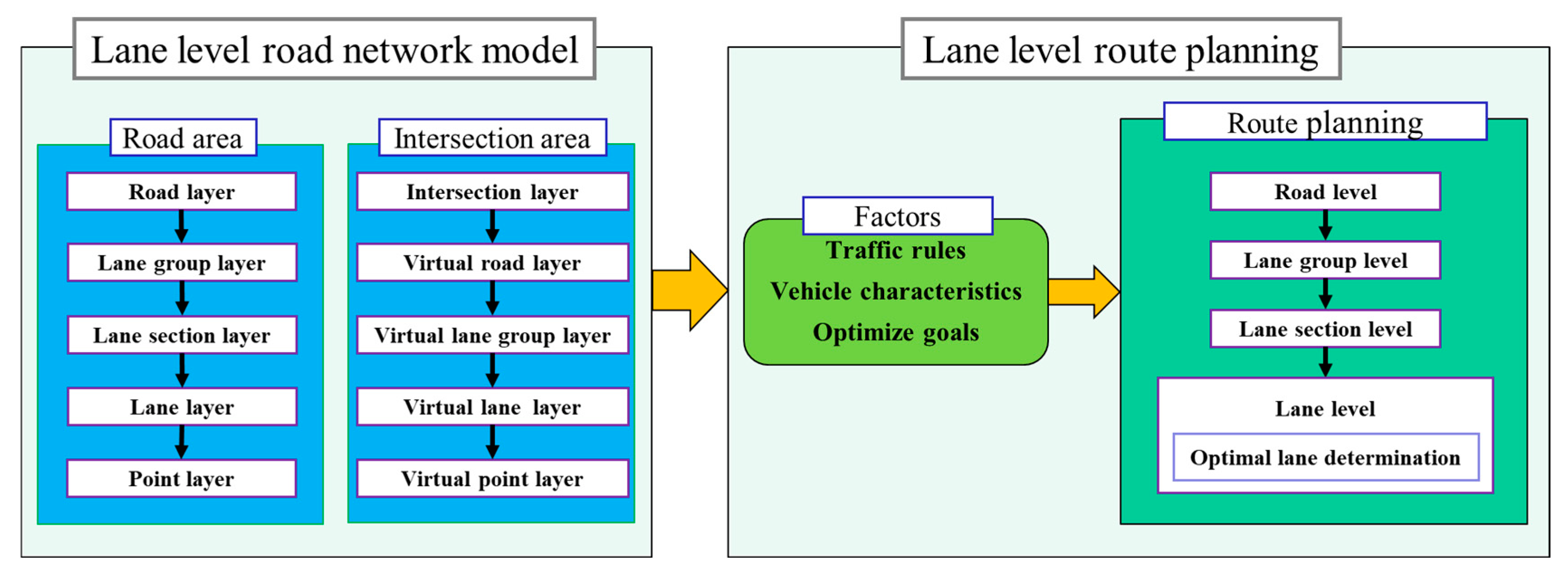
• A new road network model for lane-level route planning is proposed. The model is divided into the road and intersection areas containing five sub-layers. The model can express multiple road network structures and can facilitate more flexible, fine-grained, and efficient route planning.
• Based on the proposed road network model, an accelerated and refined lane-level route-planning method is proposed. First, a multi-level route-planning algorithm is designed for sequential planning at the road level, lane group level, lane section level, and lane level, reducing the number of nodes and edges traversed and improving routing efficiency. Then, an optimal lane determination algorithm considering traffic rules, vehicle characteristics, and optimization objectives is developed to find the optimal lanes at the lane level. The entire route-planning algorithm can remarkably improve existing search algorithms’ efficiency in searching lane-level routes and acquire optimal lanes satisfying traffic rules and vehicle characteristics on roads with different structures, including those with a constant or variable number of lanes.

The rest of this paper is organized as follows. Section 2 introduces the proposed road network model. Section 3 details the designed lane-level route-planning algorithm based on the model. Experiments are performed on simulated road networks and an actual road network to validate the route-planning algorithm, and the results and discussion are presented in Section 4. Finally, conclusions are given in Section 5.

2. Lane-Level Road Network Modeling

A new lane-level road network model, which is the foundation of the lane-level route planning elaborated upon later, is created in this section. The whole model consists of road and intersection areas containing five sub-layers, which are used to refine the structures of real roads and intersections. This multi-sub-layer modeling can express multiple variations in the road network structure and be adapted to the multi-level route-planning algorithm proposed in a later section.

The road network is expressed as follows:

$$G=(R,I)$$

(1)

where $G$ represents the complete road network, $R$ describes the road area consisting of a set of roads ${\left\{r_m\right\}}_{m=1}^{N_r}$, and $I$ is the intersection area comprising a group of intersections ${\left\{i_m\right\}}_{m=1}^{N_i}$.

2.1. Road Area

2.1.1. Road Layer

This article defines a set of lanes in the same direction on one road as a lane group. When the lanes on the road have two opposite directions, the road has two lane groups; if there is only a single direction, there is only one lane group. One road $r$ is

$$r=(LG,q_r,f,b)$$

(2)

where $LG$ is a set of lane groups ${\left\{l{g}_m\right\}}_{m=1}^{N_{lg}}$, $q_r$ represents common road attributes such as length, class, and type, and $f$ and $b$ indicate the intersection entering and leaving this road.

2.1.2. Lane Group Layer

One lane group in a road can be expressed as

$$lg=(LS,is\underset{¯}{}equal)$$

(3)

where $LS$ is a set of lane sections ${\left\{l{s}_m\right\}}_{m=1}^{N_{ls}}$, and one lane section is defined as a unit for which the number of lanes is constant. $is\underset{¯}{}equal$ can be 1 or −1, where 1 means that the lane group’s direction is the same as the forward direction defined by the road, and −1 is the opposite.

2.1.3. Lane Section Layer

One lane section in a lane group is

$$ls={\left\{l_m\right\}}_{m=1}^{N_l}$$

(4)

where ${\left\{l_m\right\}}_{m=1}^{N_l}$ is a set of lanes.

2.1.4. Lane Layer

One lane in a lane section can be characterized as

$$l=(seq,pre,suc,P_{geo},P_{attr},q)$$

(5)

where $seq$ denotes the sequence number of $l$ in $ls$; starting from the lane closest to the road centerline, the serial number increases from 1 in order. $pre$ and $suc$ define the intersection or lane connecting the start and end of $l$. $P_{geo}$ and $P_{attr}$ are point sets defined in the point layer. $q$ contains lane attributes such as the width, length and speed limit.

2.1.5. Point Layer

The point layer consists of the geometric control point set $P_{geo}$ and the attribute control point set $P_{attr}$ on each lane. $P_{geo}$ comprises the points characterizing the lane geometry. Each point $p_{geo}$ in $P_{geo}$ can be expressed as

$$p_{geo}=(n,x,y,z)$$

(6)

where $n$ is the serial number of $p_{geo}$ on the entire lane and $x,y,z$ indicate the X, Y, and Z coordinates in the ENU coordinate system.

$P_{attr}$ is a set of points on the lane markings reflecting lane property changes, which can be represented as

$$P_{attr}=(side,{\left\{p_{attr}{}^m\right\}}_{m=1}^{N_{p_{attr}}})$$

(7)

where $side$ can be “left” or “right”, indicating that the lane marking is located on the left or right side of the lane.

Each point $p_{attr}$ in $P_{attr}$ can be denoted as

$$p_{attr}=(x,y,z,s,h,type,lc)$$

(8)

where $x,y,z$ indicate the coordinates in the ENU coordinate system, $s$ is the length from the start point to this point along the lane, $h$ is the lateral distance of the point relative to the lane centerline, and $type$ indicates the point type which can take the values “start”, “end”, “lanechange”, or “typechange”. “start” and “end” represent the start and end of a lane marking, respectively. “lanechange” or “typechange” indicate that $p_{attr}$ is a demarcation point where the left or right lane marking type changes or the lane type changes. $lc$ is true if the interval of the lane marking following this point in the lane direction can allow a lane change; otherwise, it is false.

A road is taken as an example to illustrate the model in the road area, as shown in Figure 2; the road whose forward direction points to the right comprises two lane groups. $l{g}_1$ and $l{g}_2$ both have two lane sections, $l{s}_1$ and $l{s}_2$. $l{s}_1$ contains three lanes and $l{s}_2$ contains four lanes. The left and right lane markings of $l_3$ in $l{s}_2$ in $l{g}_2$ are used to illustrate the attribute control points: according to (8), the right lane marking has two attribute control points, the start and end points; since the left lane marking type changes, it has one more control point than the right lane marking, which marks the place where the lane marking type changes. For each lane marking, combining the value of $lc$ in (8) of attribute control points, the lane changeable interval can be known, facilitating the refined lane-level route-planning algorithm.

2.2. Intersection Area

2.2.1. Intersection Layer

An intersection $i$ is defined as

$$i=(VR,sig,P_{center})$$

(9)

where $VR$ represents a set of virtual roads ${\left\{v{r}_m\right\}}_{m=1}^{N_{vr}}$ that connect roads entering and leaving $i$, $sig$ indicates the intersection attributes, such as the number and position of traffic lights and the junction type, and $P_{center}$ includes the coordinates of the intersection center point.

2.2.2. Virtual Road Layer

One virtual road $vr$ can be indicated as

$$vr=(r_f,r_r,w,VLG)$$

(10)

where $r_f,r_r$ represent the roads entering or exiting the intersection and $w$ describes the passage method, including going straight, turning left, turning right, and making a U-turn.

2.2.3. Virtual Lane Group Layer

$VLG$ in (10) contains a set of virtual lane groups ${\left\{vl{g}_m\right\}}_{m=1}^{N_{vlg}}$.

One virtual lane group, $vlg$ in $VLG$, comprises all virtual lanes connecting to the same lane entering the intersection:

$$vlg=\left(seq,{\left\{v{l}_m\right\}}_{m=1}^{N_{vl}}\right)$$

(11)

where $seq$ denotes the sequence number of the lane entering the intersection and ${\left\{v{l}_m\right\}}_{m=1}^{N_{vl}}$ is a set of virtual lanes.

2.2.4. Virtual Lane Layer

One virtual lane $vl$ can be denoted as

$$vl=(l_f,l_r,P_{vl})$$

(12)

where $l_f,l_r$ represent the lanes entering or exiting the intersection.

2.2.5. Virtual Point Layer

$P_{vl}$ in (12) represents the control points approximating the possible turning trajectory of a vehicle traveling from lane $l_f$ to $l_r$. Each point $p_{vl}$ in $P_{vl}$ can be expressed as

$$p_{vl}=(n,x,y,z)$$

(13)

where $n$ is the serial number of $p_{vl}$ on the entire virtual lane and $x,y,z$ indicate the X, Y, and Z coordinates in the ENU coordinate system.

An intersection shown in Figure 3 illustrates the model in the intersection area. The figure depicts an intersection where four roads join. Each road has two lane groups represented by broad arrows on both sides of the road centerline, the direction of which indicates the lane group’s driving direction. Each lane group has only one lane section containing three lanes. The virtual roads with Road 3 as the entrance road are displayed. Only one lane entering the intersection is linked with $v{r}_1$, $v{r}_2$, or $v{r}_3$, so there is only one virtual lane group for them. $v{r}_4$, connecting Road 3 with Road 2, has two entering lanes; namely, it has two virtual lane groups. The first virtual lane group $vl{g}_1$ links with the middle lane of the lane section on Road 3. The second virtual lane group $vl{g}_2$ merges with the rightmost lane in Road 3: $v{l}_1$, $v{l}_2$, and $v{l}_3$, marked in Figure 3, are three virtual lanes in $vl{g}_2$.

2.3. Comparison with Other Map Models

In light of the preceding, the designed road area accounts for lane groups with different driving directions. The lane group considers different lane sections to represent changes in the lane number on real roads, and the change in lane type can be reflected in attribute control points. The designed intersection area contains virtual roads consisting of virtual lane groups with many virtual lanes, hierarchically representing the connections within the intersection. Therefore, the model can express multiple road network structures. The proposed model’s differences and advantages compared to the existing models are shown in

Table 1. Comparison of the proposed model with other map models.

Existing Map Models	The Proposed Model (Referred to Here as A)’s Differences and Advantages Compared to Those of the Existing Model (Referred to Here as B)
RNDF	A can express possible changes in the number of lanes on one road, but B cannot.
The model proposed by Bétaille et al. [12]	A contains the intersection model, but B ignores it, which is a basic requirement for lane-level route planning.
The model proposed by Jiang K et al. [3]	A can express possible changes in the number of lanes on one road, but B cannot.
OpenDRIVE	Compared with B, A defines lane groups and the point layer in the road area. In addition, the designed intersection area contains five sub-layers that hierarchically represent the connections within the intersection.

.

3. Lane-Level Route Planning

This section proposes an accelerated and refined lane-level route-planning method based on the established road network model. First, a multi-level route-planning algorithm is proposed and implemented in turn at the road, lane group, lane section, and lane level; the number of nodes and edges traversed can be decreased significantly to enhance routing efficiency. Then, at the lane level, an optimal lane determination algorithm considering traffic rules, vehicle characteristics, and optimization goals is designed to find the optimal lanes on roads with different configurations, including those with a constant or variable number of lanes. The route-planning method at each level is discussed in detail.

3.1. Route Planning at the Road Level

Route planning at the road level is based on the road layer and the virtual road layer, generating a feasible route with a road or an intersection as a unit. A road-level directed graph $G_R$ can be expressed as follows:

$$G_R=(V_R,E_R)$$

(14)

where $V_R$ and $E_R$ are a set of nodes comprising the intersections and edges that include roads.

When the starting point $O$ and end point $D$ are given in $G_R$, many existing graph search algorithms, such as Dijkstra and A*, can be used at this level. Finally, the result $V_R$ contains an intersection sequence to pass from the start to the end:

$$V_R=(O,i_1,\dots ,i_k,\dots ,i_n,D)$$

(15)

where $i_k$ is the $kth$ intersection in the sequence and $n$ is the number of intersections.

Then, the roads between the intersection sequence can be written as

$$E_R=(r_0,\dots ,r_k,\dots ,r_n)$$

(16)

where $r_0$ and $r_n$ are the roads where point $O$ and point $D$ are located, respectively, and $r_k$ is the road between $i_k$ and $i_{k+1}$.

3.2. Route Planning at the Lane Group Level

Route planning at the lane group level is based on the lane group layer and the virtual lane group layer.

According to the attribute $is\_equal$ in (3), the road sequence in $E_R$ can be refined into a result based on lane groups:

$$E_{LG}=(l{g}_{O-1},\dots ,l{g}_{(k-1)-k},\dots ,l{g}_{n-D})$$

(17)

where $l{g}_{O-1}$ represents the lane group between the origin $O$ and the first intersection, $l{g}_{n-D}$ represents the lane group between the $nth$ intersection and the destination $D$, $l{g}_{(k-1)-k}$ indicates the lane group between the $(k-1)th$ intersection and the $kth$ intersection, and $k=2,3,\dots ,n$.

According to (9) and (10), the intersection sequence in $V_R$ can be described based on virtual lane groups:

$$V_{VLG}=(VL{G}_1,\dots ,VL{G}_k,\dots ,VL{G}_n)$$

(18)

where $VL{G}_k$ indicates the set of virtual lane groups in the $kth$ intersection, and $k=1,2,\dots ,n$.

Figure 4 displays the route planning from the road level to the lane group level; the black lines mark the planned route. Suppose the route-planning result at the road level is the road and intersection sequence from $r_k$ to $r_{k+3}$; at the lane group level, it can be refined to the lane group sequence from $l{g}_{k-(k+1)}$ to $l{g}_{(k+3)-(k+4)}$.

3.3. Route Planning at the Lane Section Level

Route planning at the lane section level uses the correspondence between the lane group layer and the lane section layer. According to (3) and the route-planning result at the lane group level, the lane sections in the lane group $l{g}_{(k-1)-k}$ can be written as

$$L{S}_{(k-1)-k}=(l{s}_1,\dots ,l{s}_k,\dots ,l{s}_n)$$

(19)

where $l{s}_k$ is the $kth$ lane section in $l{g}_{(k-1)-k}$ and $n$ is the number of lane sections. $l{s}_1$ connects the previous intersection’s exit and $l{s}_n$ connects the entrance to the next intersection.

Then, the whole lane section sequence is

$$V_{LS}=(L{S}_{O-1},\dots ,L{S}_{(k-1)-k},\dots ,L{S}_{n-D})$$

(20)

where $L{S}_{O-1}$ represents the lane sections between the origin $O$ and the first intersection, $L{S}_{n-D}$ represents the lane sections between the $nth$ intersection and the destination $D$, $L{S}_{(k-1)-k}$ indicates the lane sections between the $(k-1)th$ intersection and the $kth$ intersection, and $k=2,3,\dots ,n$.

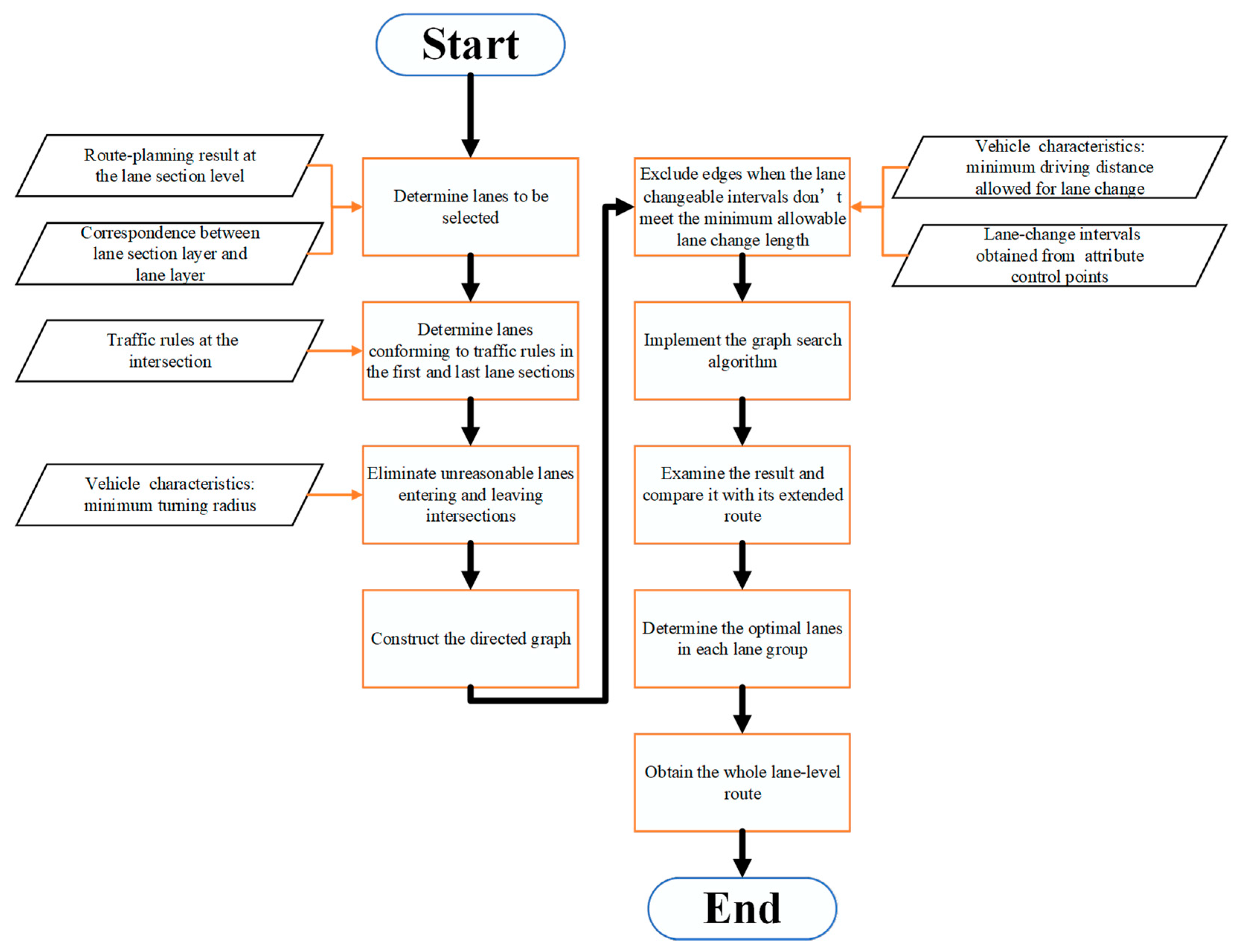
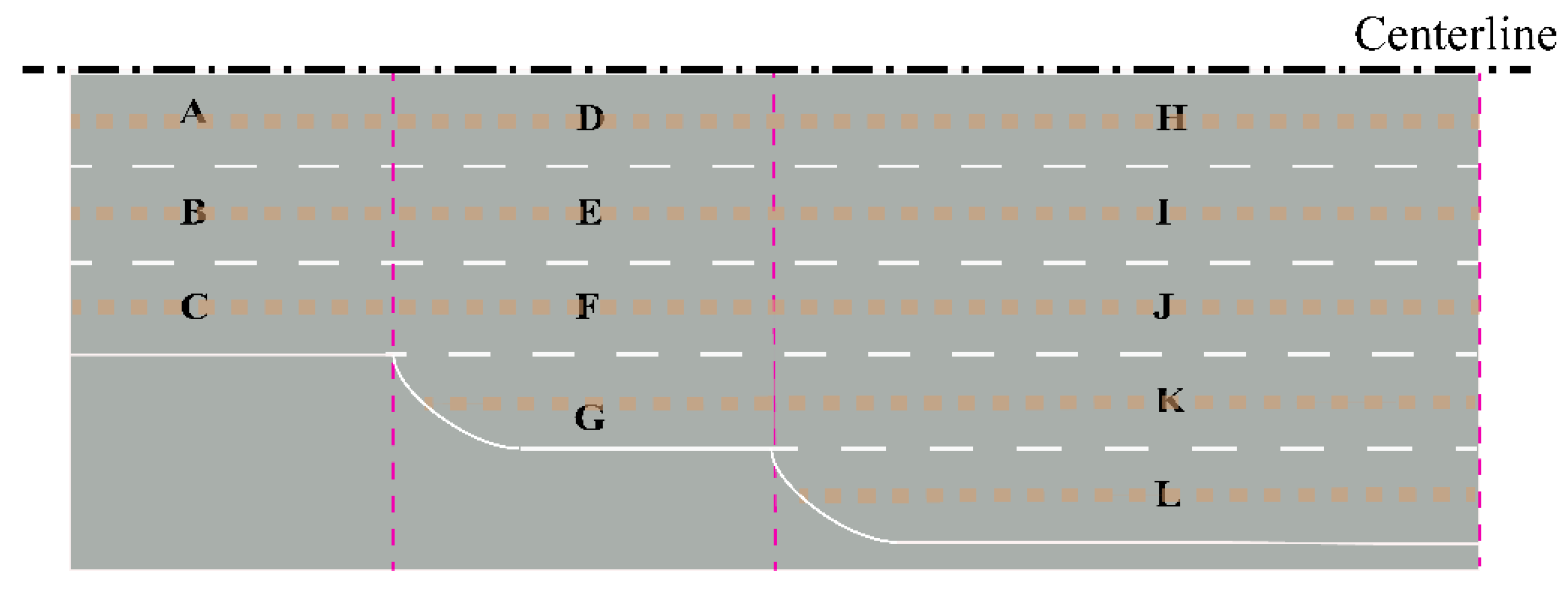
3.4. Route Planning at the Lane Level

Route planning at the lane level aims to find the optimal lanes in a sequence of lane sections in one lane group. Figure 5 displays route planning from the lane group level to the lane section level, and then to the lane level. Taking the lane group $l{g}_{(k+1)-(k+2)}$ as an example, it can be refined to the lane section sequence from $l{s}_1$ to $l{s}_2$ at the lane section level; at the lane level, the routing result is from $l_1$ to $l_2$. The route planning from the lane section level to the lane level adopts the optimal lane determination algorithm illustrated in Figure 6, which is designed as follows:

Step i: Referring to the correspondence between the lane section layer and the lane layer and the route-planning result at the lane section level, the lanes to be selected are determined.

Step ii: According to the traffic rules indicated by (12), infeasible lanes are screened out, and feasible lanes in both $l{s}_n$ in $L{S}_{(k-1)-k}$ entering $i_K$ and $l{s}_1$ in $L{S}_{k-(k+1)}$ leaving $i_K$ are determined. In other words, for each planned lane group, the lanes conforming to traffic rules in the first and last lane sections are determined.

Step iii: Vehicle characteristics are considered for the elimination of unreasonable lanes entering and leaving intersections. For example, a vehicle may not make a U-turn from the leftmost lane to the adjacent reverse lane considering the minimum turning radius of the vehicle.

Step iv: After excluding lanes that do not meet traffic rules and vehicle turning characteristics, a directed graph is constructed. The lane group displayed in Figure 7 is taken as an example. Since the lane marking between every two adjacent lanes is dashed, lane changes can occur between every two adjacent lanes. Figure 8 provides an abstraction of the directed graph; nodes represent lanes, and edges represent the transitions between every two lanes. Each node’s cost is the travel cost of driving along a single lane, and the cost of each edge perpendicular to lanes, such as that between A and B, is the travel cost of lane changing. These costs’ computing methods, which are not the focus of this study, refer to the method in Ref. [3]. The cost of each edge parallel to lanes, such as that between A and D, is zero.

Step v: The lane change intervals can be obtained according to attribute control points in the point layer. It is necessary to consider whether the lane change interval meets the minimum allowable length in combination with vehicle characteristic constraints. For example, if the lane change interval on the right lane marking of lane A is not enough for lane changing, the edge between A and B is eliminated.

Step vi: According to the predetermined first lane in $l{s}_1$ and last lane in $l{s}_n$ in Step ii and Step iii and the constructed directed graph in Step iv and Step v, a graph search algorithm, such as Dijkstra or A*, is implemented.

Step vii: The result in Step vi needs to be examined because the route can be extended at the last lane section, and the extended route could not be searched by Step vi. For example, if the result is route A-B-E-I, the route can be extended to route A-B-E-I-H-I, which means changing lanes from I to H, and then back to I in the last lane section. The costs of driving along lane I and driving from lane I to lane H and then back to I are compared. If the cost of the extended route is lower than that of the original route, the extended route replaces the result.

Step viii: After Step i–vii, the optimal lanes in each lane group are determined. The optimal lane sequence in $l{g}_{(k-1)-k}$ can be expressed as follows:

$$L_{(k-1)-k}=(l_1,\dots ,l_k,\dots ,l_n)$$

(21)

where $l_k$ is the $kth$ lane in order and $n$ is the number of lanes.

Step ix: The whole lane-level route can be obtained as

$$V_L=(L_{O-1},\dots ,L_{(k-1)-k},\dots ,L_{n-D})$$

(22)

where $L_{O-1}$ represents the lane sequence between the origin $O$ and the first intersection, $L_{n-D}$ is the lane sequence between $i_n$ and the destination $D$, $L_{(k-1)-k}$ indicates the lane sequence between $i_{k-1}$ and $i_k$, and $k=2,3,\dots ,n$.

4. Results and Discussion

A road network was first constructed to verify the lane-level routing algorithm using RoadRunner [33]. This interactive editor allows us to design 3D scenes for simulating and testing automated driving systems. Then, the OpenDrive file exported from RoadRunner was imported into SCANeR studio [34] to build an ultra-realistic virtual driving scene. SCANeR studio is a comprehensive software suite dedicated to automotive and transport simulation that provides all the tools and models necessary to create an ultra-realistic virtual world.

Figure 9 displays a constructed road network consisting of 16 intersections and 24 roads. All roads were bidirectional and comprised two lane groups; each lane group had one lane section containing three lanes. A green circle shows the host vehicle in the simulation. All of the road network parameters are given in

Table 2. Road network parameter settings.

Parameter	Value
The number of lanes in one lane section	3
The number of lane sections in one lane group	1
The number of lane groups in one road	2
Lane width	3.5 m
Intersection width	24 m
The average speed of each road: $v_{road}$ (km/h)	Randomly chosen from $\left\{80,60,40\right\}$
The average speed of each lane: $v_{lane}$ (km/h)	Inner: $v_{road}+20$; middle: $v_{road}$; outer: $v_{road}-20$
The traffic rules designed for the lanes	Inner: left; middle: forward; outer: right

. A partially enlarged intersection and corresponding virtual lanes in the intersection are displayed in Figure 10.

Figure 11 presents an abstraction of the simulated road network and the planned route from A to B. There are 16 vertices representing intersections and 24 edges representing roads. The average road speed is marked next to the road edge. The value on the coordinate axis shows the length of each edge. Taking the shortest total time as the goal, the route from vertex A on the lower left to vertex B on the upper right was planned using the algorithm proposed, and the red lines indicate the planned route. The average speed of the roads through the planned route is high, and the route meets the shortest time goal at the road level. The circles on the right side depict the lane-level details inside the indicated junctions: four roads enter the junction; the arrows represent the lanes’ driving directions, the dotted lines represent the roads’ centerlines, and the red lines show the planned route in the junction.

Two junctions are chosen to illustrate the lane-level routing results. At Junction 1, since a vehicle on the road left of the intersection must turn left when entering the intersection, it will travel in the inner lane, which meets the traffic regulations; on the other hand, after leaving the intersection, the inner lane with a high average speed is chosen, which satisfies the goal of achieving the shortest travel time. Similarly, at Junction 2, the vehicle will travel straight from the middle lane to the inner lane. This result reveals that the proposed algorithm based on the map model successfully chose the correct lanes on roads with a constant number of lanes to meet both the traffic rules and the routing goal; namely, the algorithm can find the optimal lane-level route in a road network.

Another test is shown in Figure 12, where the route from lane C to lane D is planned. To illustrate the main route-planning problem in this paper, it is assumed that the minimum turning radius, which can be estimated according to vehicle characteristics, is 8 m. The planned route can be obtained using the method in Ref. [3], and this study, it is represented by the green or red lines. We can see that the route planned by Ref. [3] goes from lane C to lane D directly; however, the minimum turning radius is larger than the two-lane width, such that the vehicle cannot directly U-turn from C to D; hence, the result is not feasible. In contrast, the route developed using the method in this study first includes a U-turn from C to E and then involves a change of lanes from E to D; although this route has a higher cost, it fits the vehicle turning characteristics. Therefore, the algorithm in this study can obtain a reasonable route considering vehicle turning characteristics, meeting the needs of practical applications.

Another road network, displayed in Figure 13, was constructed to verify the optimal lane determination algorithm at the lane level. The minimum length for lane changing, considering vehicle characteristics, was set to 10 m, so the interval CD was not available for a lane change; the interval AB and EF were allowed. The traffic rules designed on Lane 3–5 entering the intersection were left turn, forward and right turn, and forward and right turn, respectively. The average speeds in Lane 1–5 were 50 km/h, 30 km/h, 30 km/h, 60 km/h, and 30 km/h, respectively.

First, the lanes to be selected were determined according to Steps i–iii of the optimal lane determination algorithm at the lane level; the lanes chosen from $l{s}_1$ were Lane 1 and Lane 2, and the lanes chosen from $l{s}_2$ were Lane 4 and Lane 5. In contrast, Lane 3 was excluded due to the traffic rule. According to Steps iv–v, the directed graph was created as shown in Figure 14. Figure 15 illustrates all possible routes. After Step vi, Route 1 (Lane 1–Lane 4) in Figure 15a was chosen. Then, according to Step vii, Route 2 (Lane 1–Lane 4–Lane 3–Lane 4) in Figure 15a, which was the extended route of Route 1, was compared with Route 1. Finally, Route 1, with a lower cost than Route 2, was chosen as the optimal lane-level route. At the same time, the costs of all possible routes were calculated. By comparison, the cost of Route 1 was the lowest, which verified the correctness of the optimal lane determination algorithm.

This test demonstrates that the optimal lane determination algorithm could find the optimal lanes while satisfying traffic rules and vehicle characteristics on roads with a variable number of lanes. In contrast, the algorithm in Ref. [3] subdivides the road into a constant number of lanes and lacks the adaptability to this road structure; however, this road structure may result in the creation of an increased number of possible routes that need to be considered before one is chosen.

Whether the road has a constant or variable number of lanes, the directed graph can be constructed at the lane level. For example, if the lane number is constant at three, a simple directed graph consisting of three vertices and two edges can be constructed; if the road has a variable number of lanes, a more complex directed graph can be constructed. Then, the existing graph search algorithm can be applied to find the optimal route. The algorithm in Ref. [3] did not consider the lane sections as defined in this study, it could not adapt to the changing internal structure of the road. In addition, the lane change intervals are not considered in Ref. [3], meaning that the produced route may not be feasible. The tests, which assign different average speeds to different road and lanes, are mainly conducted to verify that the proposed algorithm can adapt to road networks with different structures while meeting the traffic rules and vehicle characteristics. In addition, the goal for the shortest time is satisfied under relative static conditions. The variable traffic conditions, which may influence the edges’ costs, are not considered here; however, some existing algorithms considering the real-time traffic conditions can be applied at the road level and lane level and improve the practicability in the actual traffic conditions, which needs further research in the future.

From the previous section, it can be inferred that the suggested route-planning algorithm can determine the optimal lanes on roads with different configurations, including those with a constant or variable number of lanes, while satisfying the need for the shortest time, as well as the requirements for traffic regulations and vehicle characteristics, which allows the planned route to match the actual vehicle navigation needs.

Next, the increasingly intricate road networks depicted in Figure 16 were built to assess the algorithm’s efficiency improvement in road networks of different sizes. To confirm the improved efficiency of our proposed algorithm, we compared the routing time of different routing algorithms, including direct lane-level route planning using the existing graph search algorithm, the route-planning method proposed in Ref. [3] and the route-planning algorithm proposed in this study, in the road networks detailed in Figure 9 and Figure 16.

Direct lane-level route planning searches the lane-level route directly on the road network. Figure 17 illustrates a road network comprising one road and an intersection. Following the directed graph abstraction of the road network (Figure 18), the direct routing can perform the existing graph search algorithm to search the lane-level route.

We implemented the algorithms in C++, maintaining consistency in the hardware setup and data structure and varying the algorithms themselves. To verify the improvement in efficiency in the proposed algorithm over the existing graph search algorithm, the A* algorithm was taken as an example.

Table 3. Time costs of different routing methods in three simulated road networks with different scales.

Number of Lanes	Routing Method	$\mathbf{Time}\left(\mathsf{\mu }\mathbf{s}\right)$	Time Saved (%)
288	Direct lane-level route planning	61
	Lane-level route planning proposed in Ref. [3]	38	37.7
	Lane-level route planning in this study	20	67.2
705	Direct lane-level route planning	383
	Lane-level route planning proposed in Ref. [3]	77	79.9
	Lane-level route planning in this study	35	90.1
10,088	Direct lane-level route planning	7832
	Lane-level route planning proposed in Ref. [3]	535	93.2
	Lane-level route planning in this study	304	96.1

compares different routing methods, and the time saved is relative to the time spent using direct route planning based on A*. Both the algorithm in this study and the process in Ref. [3] can improve the efficiency compared with direct route planning; however, the algorithm in this study has higher efficiency for both small or large networks, and the improvement in efficiency becomes more remarkable as the scale of the road network grows.

In this test, the A* algorithm was utilized at the road level in the proposed algorithm, which is consistent with Ref. [3], so the efficiency difference between this study and Ref. [3] is brought about by different hierarchical structures. The proposed algorithm directly eliminates the candidate lanes with different directions through the defined lane groups, which further reduces the search space compared to the method described in Ref. [3], which direct maps from roads to lanes, and thus speeds up the search speed. This proposed method is generally applicable to various road networks and can effectively reduce the search space of various algorithms, so the algorithm proposed in this paper can effectively improve the efficiency of existing algorithms when used for lane-level route planning. Although the test did not consider the changing traffic, which mainly affects the edges’ cost, the search space can also be reduced by the proposed algorithm in real-time changing traffic conditions, so it can be inferred that the existing algorithms’ efficiency can also be improved in dynamic traffic conditions. In conclusion, this simulation test validated the proposed method as having better efficiency in supporting lane-level navigation than the direct and past hierarchical routing methods.

The test was also conducted on the physical road network at Changchun, China, to validate the effectiveness of route-planning algorithm. High-precision point cloud maps were initially retrieved using the probe vehicle presented in Figure 19. Since LiDAR delivers a high-resolution 360-degree environment, the entire road geometry can be captured. Based on the results of the collected LiDAR data, a high-precision point cloud map of the test site was built first, as shown in Figure 20a, and then a lane-level electronic map was established, as shown in Figure 20b.

The red lines in Figure 21 demonstrate the routing outcome. It is clear that the proposed method picked the correct lanes to arrive at the destination, demonstrating that the method can obtain reasonable routes on the physical road network.

Table 4. Time costs of different routing methods in a real road network.

Number of Lanes	Routing Method	$\mathbf{Time}\left(\mathsf{\mu }\mathbf{s}\right)$	Time Saved (%)
323	Routing algorithm of Apollo	132
	Routing algorithm in this study	29	78.0

illustrates the time costs of the Apollo routing method [35] and the proposed algorithm. We can see that the proposed algorithm improved routing efficiency by 78.0% compared with the Apollo method, so the proposed algorithm can better meet the real-time requirements of autonomous driving.

5. Conclusions

In this study, which was aimed at providing better support for navigation systems in autonomous vehicles, an efficient lane-level route-planning algorithm based on a new lane-level road network model is proposed, which is manifested in the following aspects:

• A new road network model for lane-level route planning is proposed. The whole model is divided into the road area and the intersection area, containing five sub-layers, refining the structures of real roads and intersections. On the one hand, this multi-sub-layer modeling can express variations in the road network structure; on the other hand, it facilitates the proposed multi-layer route-planning algorithm, improving the overall routing efficiency.
• Based on the proposed road network model, an accelerated and refined lane-level route-planning method is proposed. First, a multi-layer route-planning algorithm is designed to plan sequentially at the road level, lane group level, lane section level, and lane level, resulting in remarkable improvements in routing efficiency, especially in large-scale road networks. Then, an optimal lane determination algorithm is developed at the lane level to find the optimal lanes while satisfying traffic rules and vehicle characteristics. The entire route-planning method can be seen as a framework compatible with existing algorithms, which means the existing graph search methods can be applied at the road and lane level to take advantage of the progress of existing research, and the routing efficiency can be dramatically improved compared to that of direct route planning using the graph search methods at the lane level. In addition, the proposed algorithm can better adapt to the changing road network structure and yield optimal lanes on roads with different configurations, including those with a constant or variable number of lanes. Tests were performed on simulated road networks and an actual road network. The results demonstrate the effectiveness, broader adaptability, and higher efficiency of the proposed algorithm compared with direct route planning, past hierarchical route planning, and the Apollo route-planning method. In particular, the efficiency can be improved by up to 96.1% compared with direct route planning using the graph search methods at the lane level. This study is complementary to existing studies and better supports autonomous vehicle navigation.

This proposed algorithm can effectively improve the efficiency of existing algorithms when used for lane-level route planning by reducing the search space. However, it is more theoretical than practical due to the lack of consideration of the influence of real driving conditions. Although it can be inferred that the search space can also be reduced by the proposed algorithm in real-time changing traffic conditions, to increase the utility of the method in practical navigation applications, further research will consider the traffic conditions, weather, and other factors that influence the actual travel costs in order to obtain the optimal route in practice. At the same time, considering these factors increases the complexity of routing, and a balance between routing complexity and efficiency will be considered in the future.

References

1. Groves, P.D. Principles of GNSS, Inertial, and Multisensor Integrated Navigation Systems, 2nd ed.; Artech House: London, UK, 2013; 776p, ISBN 978-1-60807-005-3. [Google Scholar]
2. Brügger, A.; Richter, K.-F.; Fabrikant, S.I. How does navigation system behavior influence human behavior? Cogn. Res. Princ. Implic. 2019, 4, 1. [Google Scholar] [CrossRef] [PubMed] [Green Version]
3. Jiang, K.; Yang, D.; Liu, C.; Zhang, T.; Xiao, Z. A flexible multi-layer map model designed for lane-level route planning in autonomous vehicles. Engineering 2019, 5, 305–318. [Google Scholar] [CrossRef]
4. Gyagenda, N.; Hatilima, J.V.; Roth, H.; Zhmud, V. A review of GNSS-independent UAV navigation techniques. Robot. Auton. Syst. 2022, 152, 104069. [Google Scholar] [CrossRef]
5. Zhang, J.; Wen, W.; Huang, F.; Wang, Y.; Chen, X.; Hsu, L.-T. GNSS-RTK Adaptively Integrated with LiDAR/IMU Odometry for Continuously Global Positioning in Urban Canyons. Appl. Sci. 2022, 12, 5193. [Google Scholar] [CrossRef]
6. Upadhyay, V.; Balakrishnan, M. Monocular Localization Using Invariant Image Feature Matching to Assist Navigation. In Computers Helping People with Special Needs, Proceedings of the 18th International Conference, ICCHP-AAATE 2022, Lecco, Italy, 11–15 July 2022; Proceedings, Part I; Springer International Publishing: Cham, Switzerland, 2022; pp. 178–186. [Google Scholar]
7. Zhang, Y.; Wang, L.; Jiang, X.; Zeng, Y.; Dai, Y. An efficient LiDAR-based localization method for self-driving cars in dynamic environments. Robotica 2022, 40, 38–55. [Google Scholar] [CrossRef]
8. Zheng, L.; Li, B.; Yang, B.; Song, H.; Lu, Z. Lane-level road network generation techniques for lane-level maps of autonomous vehicles: A survey. Sustainability 2019, 11, 4511. [Google Scholar] [CrossRef] [Green Version]
9. Sivaraman, S.; Trivedi, M.M. Dynamic probabilistic drivability maps for lane change and merge driver assistance. IEEE Trans. Intell. Transp. Syst. 2014, 15, 2063–2073. [Google Scholar] [CrossRef]
10. Schindler, A.; Maier, G.; Janda, F. Generation of high precision digital maps using circular arc splines. In Proceedings of the IEEE Intelligent Vehicles Symposium, Alcala de Henares, Spain, 3–7 June 2012; pp. 246–251. [Google Scholar]
11. Guo, C.; Meguro, J.I.; Kojima, Y.; Naito, T. Automatic lane-level map generation for advanced driver assistance systems using low-cost sensors. In Proceedings of the IEEE International Conference on Robotics and Automation, Hong Kong, China, 31 May–7 June 2014; pp. 3875–3982. [Google Scholar]
12. Bétalille, D.; Toledo-Moreo, R. Creating enhanced maps for lane-level vehicle navigation. IEEE Trans. Intell. Transp. Syst. 2010, 11, 786–798. [Google Scholar] [CrossRef]
13. Zhang, T.; Arrigoni, S.; Garozzo, M.; Yang, D.; Cheli, F. A lane-level road network model with global continuity. Transp. Res. Part C Emerg. Technol. 2016, 71, 32–50. [Google Scholar] [CrossRef]
14. Jo, K.; Sunwoo, M. Generation of a precise roadway map for autonomous cars. IEEE Trans. Intell. Transp. Syst. 2014, 15, 925–937. [Google Scholar] [CrossRef]
15. Gwon, G.-P.; Hur, W.-S.; Kim, S.-W.; Seo, S.-W. Generation of a precise and efficient lane-level road map for intelligent vehicle systems. IEEE Trans. Veh. Technol. 2016, 66, 4517–4533. [Google Scholar] [CrossRef]
16. DARPA. Urban Challenge: Route Network Definition File (RNDF) and Mission Data File (MDF) Formats; Defense Advanced Research Projects Agency: Arlington, VA, USA, 2007.
17. NDS Open Lane Model 1.0 Release. Available online: http://www.openlanemodel.org/ (accessed on 19 June 2019).
18. Dupuis, M.; Hekele, E.; Biehn, A. OpenDRIVE® v1.4 Format Specification; VIRES Simulationstechnologie GmbH: Bad Aibling, Germany, 2015. [Google Scholar]
19. Zhu, Z.; Li, L.; Wu, W.; Jiao, Y. Application of improved Dijkstra algorithm in intelligent ship path planning. In Proceedings of the Chinese Control and Decision Conference, Kunming, China, 22–24 May 2021; pp. 4926–4931. [Google Scholar]
20. Pandika, I.K.L.D.; Irawan, B.; Setianingsih, C. Apllication of optimization heavy traffic path with Floyd-Warshall algorithm. In Proceedings of the International Conference on Control Electronics Renewable Energy and Communications, Bandung, Indonesia, 5–7 December 2018; pp. 57–62. [Google Scholar]
21. Candra, A.; Budiman, M.A.; Hartanto, K. Dijkstra’s and AStar in finding the shortest path: A tutorial. In Proceedings of theInternational Conference on Data Science, Artificial Intelligence and Business Analytics, Medan, Indonesia, 16–17 July 2020; pp. 28–32. [Google Scholar]
22. Jangra, R.; Kait, R. Analysis and comparison among ant system ant colony system and Max-Min ant system with different parameters setting. In Proceedings of the International Conference on Computational Intelligence & Communication Technology, Ghaziabad, India, 9–10 February 2017; pp. 1–4. [Google Scholar]
23. Xu, Z.; Liu, X.; Chen, Q. Application of improved Astar algorithm in global path planning of unmanned vehicles. In Proceedings of the Chinese Automation Congress, Hangzhou, China, 22–24 November 2019; pp. 2075–2080. [Google Scholar]
24. Lee, M.; Yu, K. Dynamic path planning based on an improved ant colony optimization with genetic algorithm. In Proceedings of the IEEE Asia-Pacific Conference on Antennas and Propagation, Auckland, New Zealand, 5–8 August 2018; pp. 1–2. [Google Scholar]
25. Jiang, C.; Fu, J.; Liu, W. Research on vehicle routing planning based on adaptive ant colony and particle swarm optimization algorithm. Int. J. Intell. Transp. Syst. Res. 2021, 19, 83–91. [Google Scholar] [CrossRef]
26. Lan, X.; Lv, X.; Liu, W.; He, Y.; Zhang, X. Research on robot global path planning based on improved A-star ant colony algorithm. In Proceedings of the 2021 IEEE 5th Advanced Information Technology, Electronic and Automation Control Conference (IAEAC), Chongqing, China, 12–14 March 2021; pp. 613–617. [Google Scholar]
27. Rossi, F.; Zhang, R.; Hindy, Y.; Pavone, M. Routing autonomous vehicles in congested transportation networks: Structural properties and coordination algorithms. Auton. Robot. 2018, 42, 1427–1442. [Google Scholar] [CrossRef] [Green Version]
28. Zheng, W.; Thangeda, P.; Savas, Y.; Ornik, M. Optimal routing in stochastic networks with reliability guarantees. In Proceedings of the IEEE International Intelligent Transportation Systems Conference (ITSC), Indianapolis, IN, USA, 19–22 September 2021; pp. 3521–3526. [Google Scholar]
29. Bailey, C.; Jones, B.; Clark, M.; Buck, R.; Harper, M. Electric Vehicle Autonomy: Realtime Dynamic Route Planning and Range Estimation Software. In Proceedings of the 2022 IEEE 25th International Conference on Intelligent Transportation Systems (ITSC), Macau, China, 8–12 October 2022; pp. 2696–2701. [Google Scholar]
30. Bucher, D.; David, J.; Raubal, M. A heuristic for multi-modal route planning. In Progress in Location-Based Services 2016; Springer: Cham, Switzerland, 2017; pp. 211–229. [Google Scholar]
31. Dibbelt, J.; Strasser, B.; Wagner, D. Customizable contraction hierarchies. J. Exp. Algorithmics 2016, 21, 1–49. [Google Scholar] [CrossRef] [Green Version]
32. Wu, Y.; Song, W.; Cao, Z.; Zhang, J.; Lim, A. Learning improvement heuristics for solving routing problems. IEEE Trans. Neural Netw. Learn. Syst. 2021, 33, 5057–5069. [Google Scholar] [CrossRef] [PubMed]
33. Kanakagiri, A. Development of a Virtual Simulation Environment for Autonomous Driving Using Digital Twins. Ph.D. Thesis, Technische Hochschule Ingolstadt, Ingolstadt, Germany, 2021. [Google Scholar]
34. That, T.N.; Casas, J. An integrated framework combining a traffic simulator and a driving simulator. Procedia Soc. Behav. Sci. 2011, 20, 648–655. [Google Scholar] [CrossRef] [Green Version]
35. Available online: https://github.com/ApolloAuto/apollo (accessed on 12 October 2022).
Figure 1. The main research content of this study.
Wevj 14 00098 g001
Figure 2. A road used to illustrate the model. The marked numbers are the sequence numbers of lanes.
Wevj 14 00098 g002
Figure 3. An intersection used to illustrate the model.
Wevj 14 00098 g003
Figure 4. The route planning from the road level to the lane group level.
Wevj 14 00098 g004
Figure 5. The route planning from the lane group level to the lane section level, and then to the lane level.
Wevj 14 00098 g005
Figure 6. The flowchart of the optimal lane determination algorithm.
Wevj 14 00098 g006
Figure 7. A lane group is shown, which comprises three lane sections that contain three, four, and five lanes, respectively. Each lane is identified by a capital letter from A to L.
Wevj 14 00098 g007
Figure 8. The directed graph abstracted from the lane group shown in Figure 7. The arrows indicate the travel directions. Two-way arrows represent mutual access; for example, the two-way arrow between D and E indicates that the vehicle can move from D to E and E to D.
Wevj 14 00098 g008
Figure 9. The road network and the corresponding driving scene. (a) The road network constructed by RoadRunner. (b) The driving scene created using SCANeR studio.
Wevj 14 00098 g009
Figure 10. An intersection and corresponding virtual lanes. (a) An intersection and four connecting roads are shown. (b) The virtual lanes in the intersection shown in (a) are displayed.
Wevj 14 00098 g010
Figure 11. Abstraction of the simulated road network. The red lines show the planned route. A and B are the start and end of the route.
Wevj 14 00098 g011
Figure 12. The constructed road network includes four roads and an intersection. Each road has six lanes, each with a width of 3.5 m. The lanes on the left road are represented by A–F. The average speed on all six lanes is set to be the same. Lane A, B, and C enter the intersection, and Lane D, E, and F exit. The traffic rules on Lane C allow for left turns and U-turns. The lane-level route from Lane C to Lane D is demonstrated. The green route is obtained using the method in Ref. [3].
Wevj 14 00098 g012
Figure 13. The road had two lane sections, l s 1 and l s 2 , containing two and three lanes numbered from 1 to 5. A–F are attribute control points stored in the point layer, and the dotted line between the two points indicates that lane changes are allowed.
Wevj 14 00098 g013
Figure 14. The directed graph of Figure 13.
Wevj 14 00098 g014
Figure 15. (a). Three possible routes with Lane 1 as the start lane. (b). Three possible routes with Lane 2 as the start lane.
Wevj 14 00098 g015
Figure 16. Two road networks were constructed, and the length of each road was randomly set. (a) A road network containing 6 roads in horizontal and vertical directions. (b) A road network containing 21 roads in horizontal and vertical directions.
Wevj 14 00098 g016
Figure 17. A road (green) with one lane group comprising two lane sections entering an intersection (orange). The lanes are treated as edges represented as A–G, the start and end nodes of which are expressed with P.
Wevj 14 00098 g017
Figure 18. The abstracted directed graph. Blue dots represent nodes, and red lines represent edges.
Wevj 14 00098 g018
Figure 19. Vehicle for recording mapping data, equipped with RTK-GPS, LiDAR, and cameras.
Wevj 14 00098 g019
Figure 20. (a) Point cloud map of the test site at Changchun, China. (b) Lane-level electronic map of the test site at Changchun, China.
Wevj 14 00098 g020
Figure 21. The blue lines represent the lane centerlines in the map demonstrated in Figure 20, and the red lines highlight the planned route.
Wevj 14 00098 g021