
Estimation of Public Charging Demand Using Cellphone Data and Points of Interest-Based Segmentation


Abstract
1. Introduction
2. Literature Review
2.1. Charging Type Independent Approaches
2.1.1. Demand Estimation
2.1.2. Optimization Models
2.2. Charging Type Dependent Approaches
2.3. A New Approach
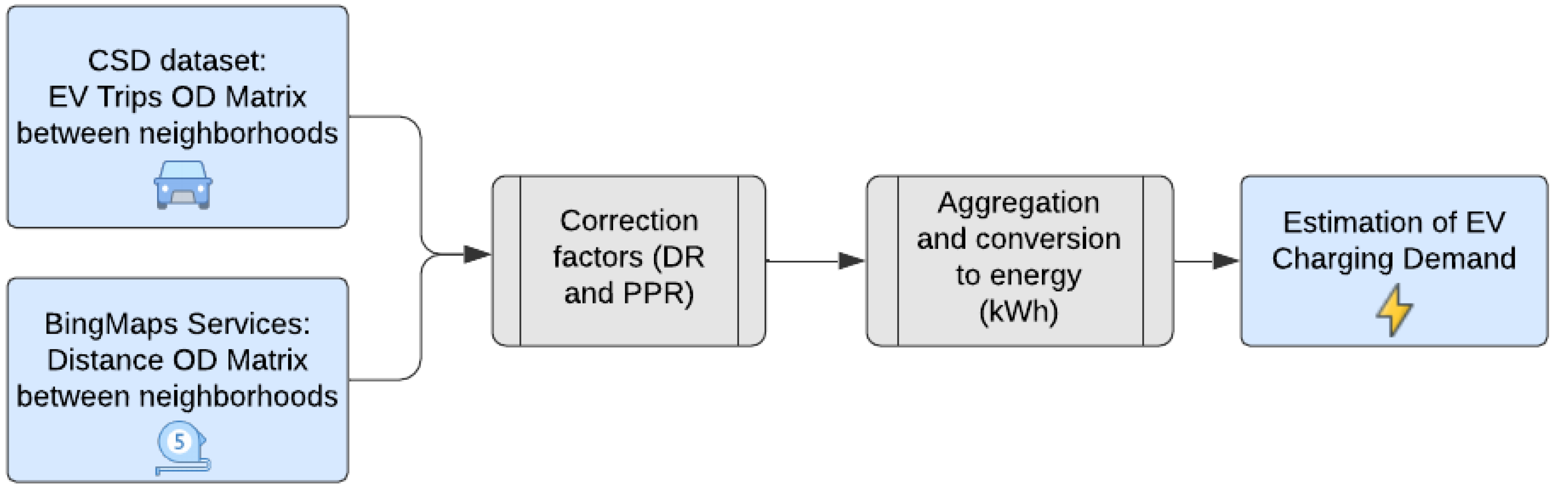
3. Materials and Methods
3.1. Demand Estimation
3.1.1. Methodology Overview
3.1.2. Origin–Destination Matrix
3.1.3. Correction Factors
3.1.4. Conversion to Energy
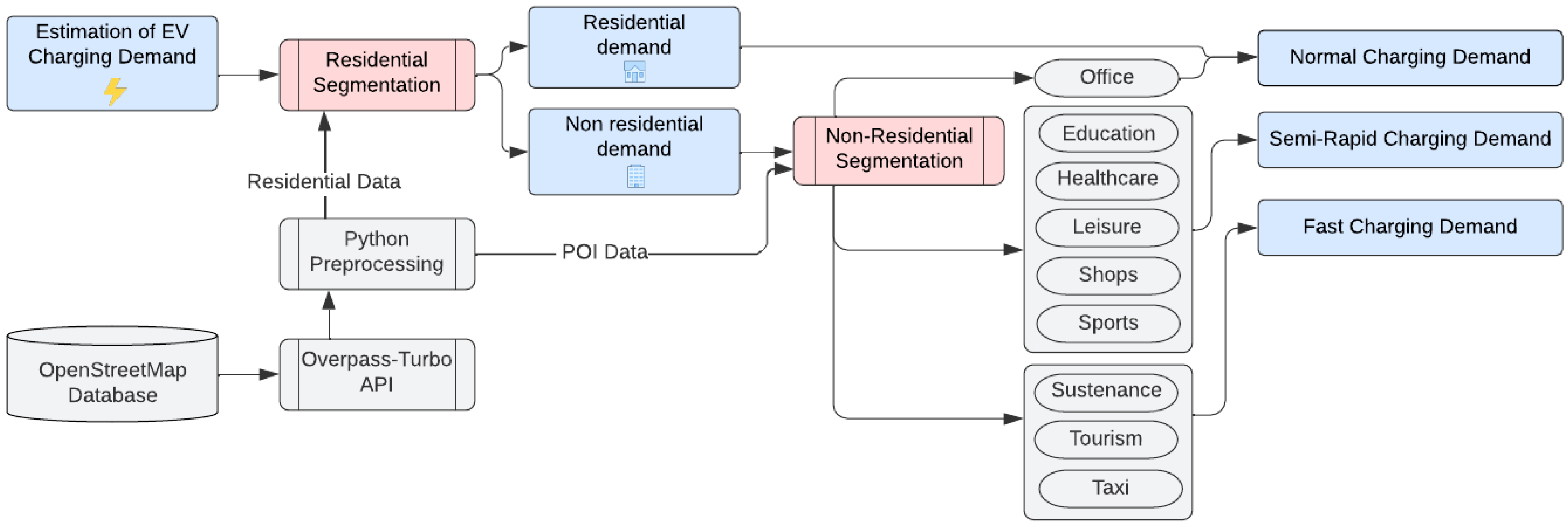
3.2. Demand Segmentation
3.2.1. Methodology Overview
3.2.2. Residential Segmentation
3.2.3. Non Residential Segmentation
4. Results
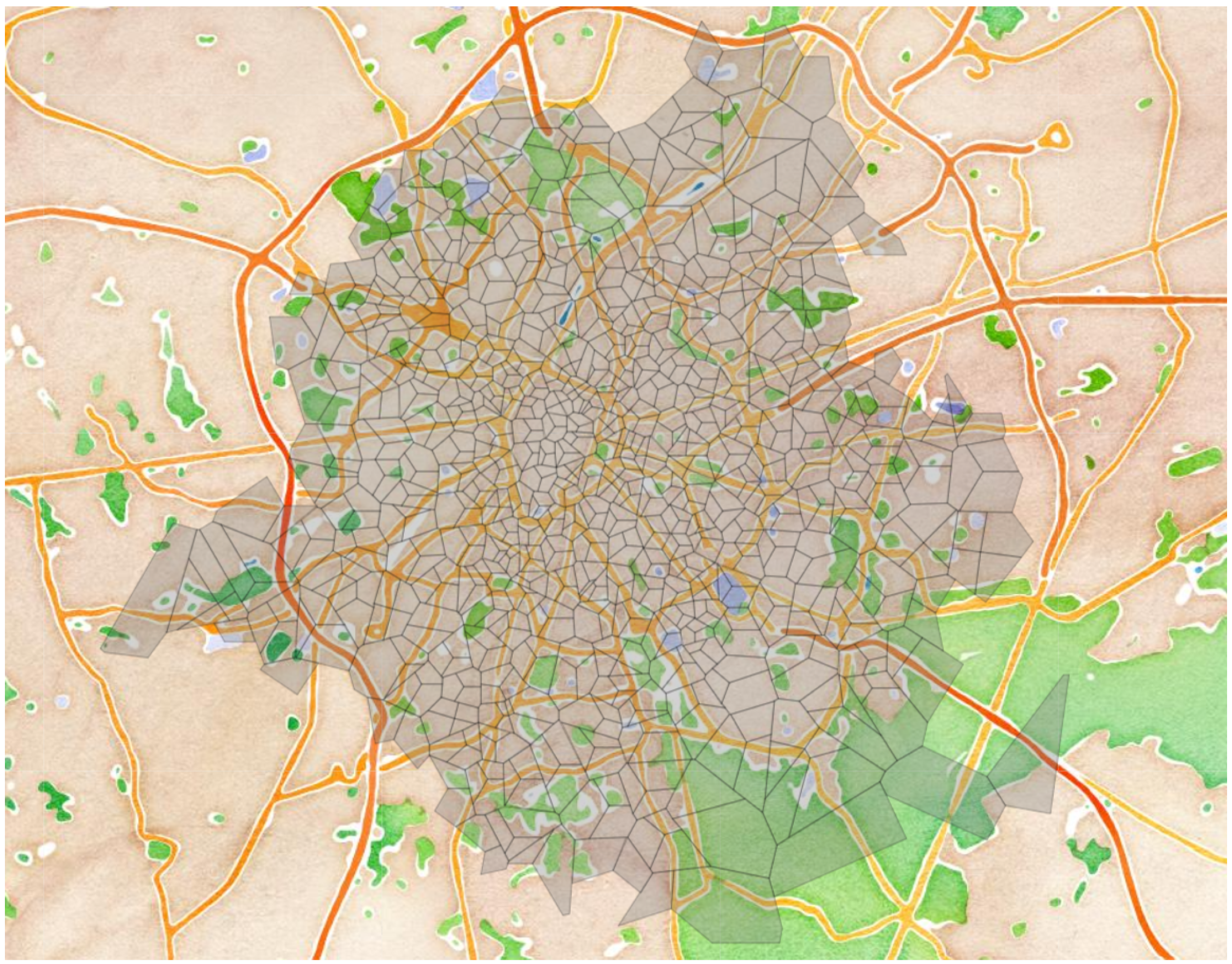
4.1. Case Study Of Brussels
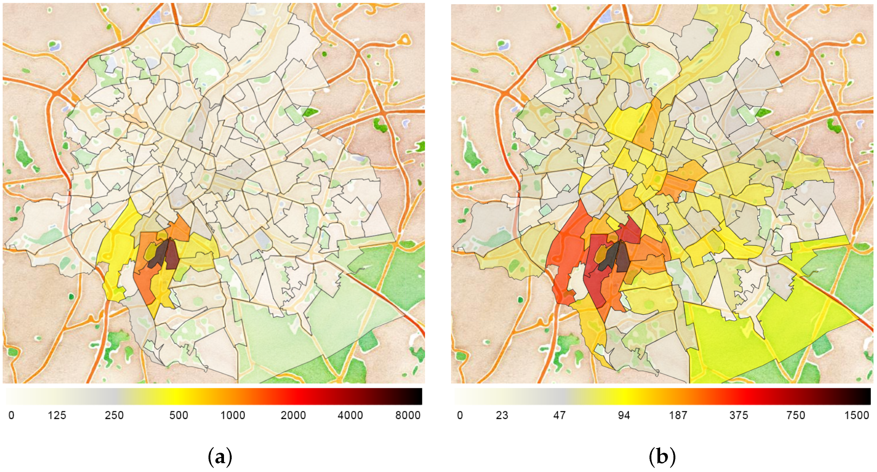
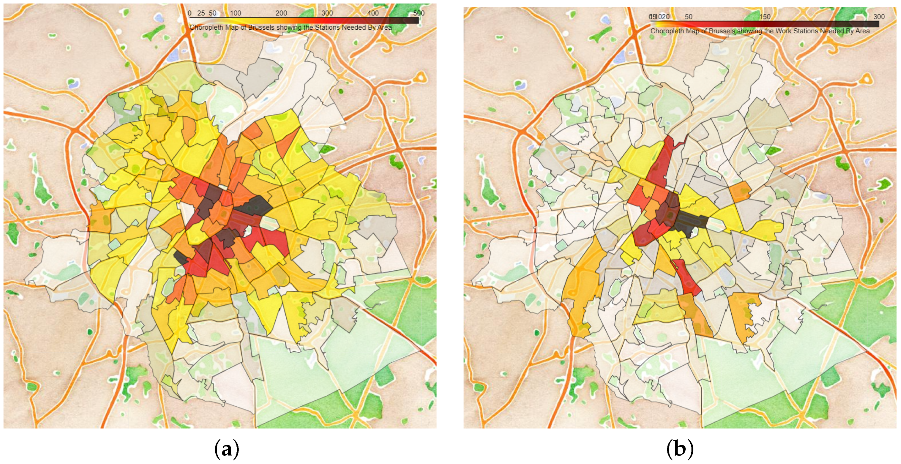
4.1.1. Estimation Results
 ,
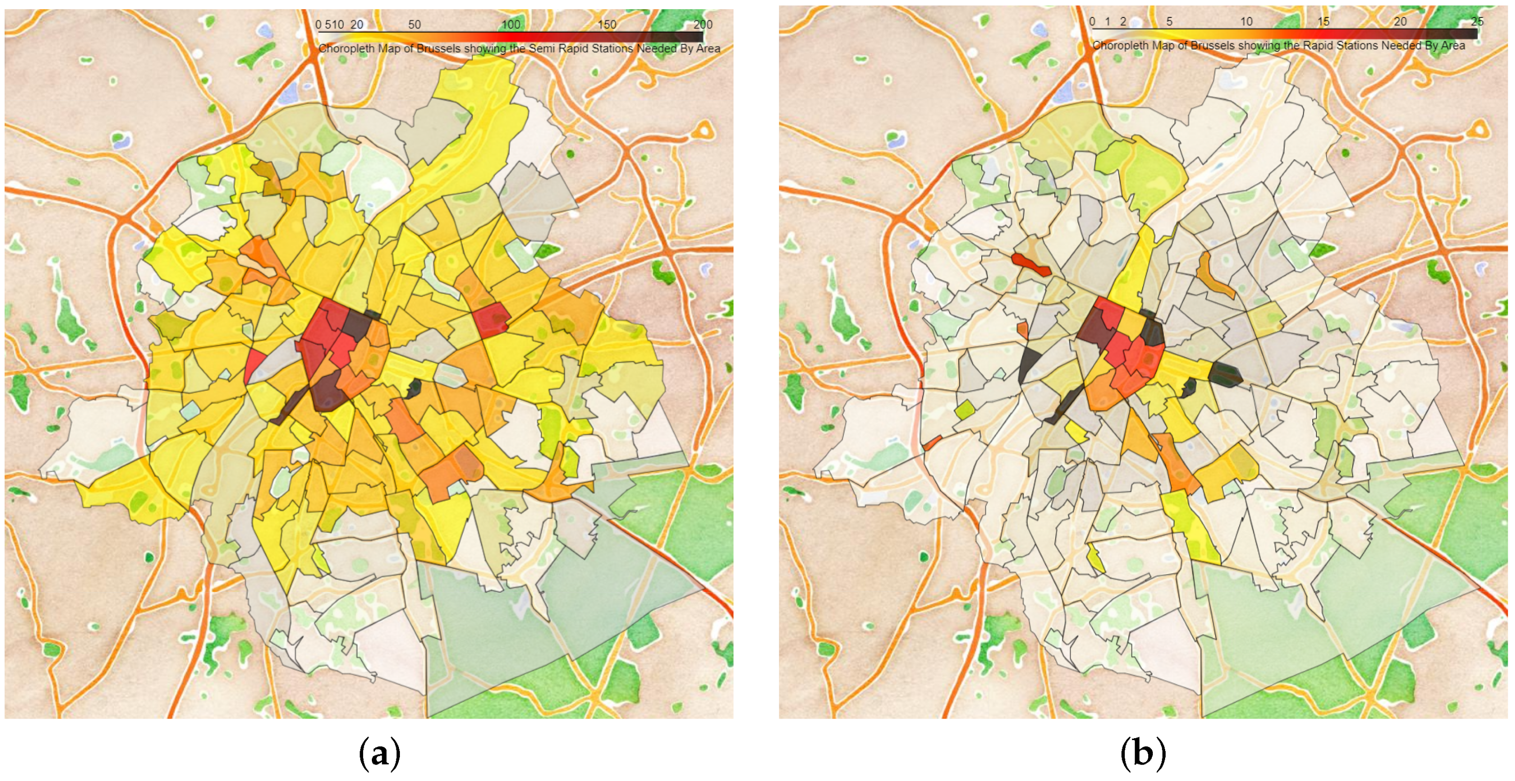
, ) neighborhoods in the south are both highly residential. Nevertheless, there is a significant charging demand difference between them, which may, at first, seem paradoxical. The left one, Homborch, exceeds 5.2 MWh (around 50 stations needed), whereas the right one, Viver d’Oie, has the lowest charging demand of all districts, 0 MWh. How is this difference possible? Vivier d’Oie accommodates mainly large detached houses, which leads to a PPR close to 1 and makes it independent from public infrastructures. On the contrary, Homborch accommodates subsidized housings with a low PPR, which justifies the higher density of public chargers. Note that a null charging demand for Viver d’Oie is probably unrealistic as under-estimated. The demand is set to 0 because the PPR means more private parking lots than households. This extreme example highlights the importance of the PPR. If we want the chargers to be ultimately homogeneously dispatched around the city, the PPR value may be capped at 95% to prevent such situations.
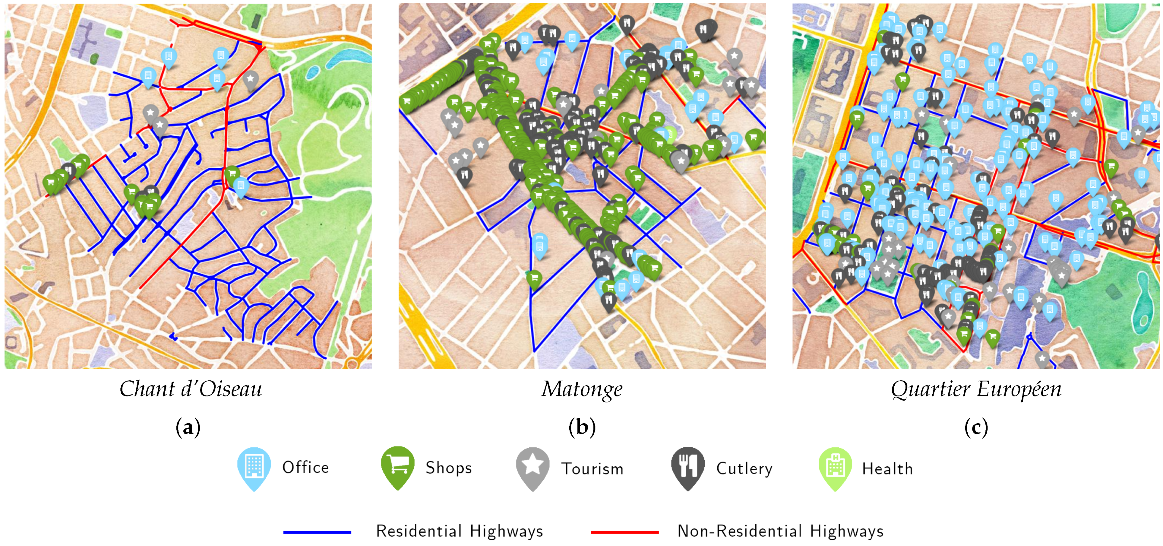
 ) in the city center represents the Quartier Européen, a working district. Its high charging demand makes sense, but, as we shall show in Section 4.1.2, companies may partly support it. The two light-blue apartment (
 ) icons show residential areas where many people live in apartments with a very low PPR Ratio. The light-green cross (
 ) icon represents the Delta neighborhood, hosting the city’s largest hospital. The purple-train icon (
 ) shows a bustling district that includes one of the city’s main train stations in Brussels. In such areas, it is understandable that charging needs will be higher. Finally, the green-tree icons (
 ) symbolize poorly populated district, such as parks, forests, or cemeteries, which explains the poor (or null) charging demand (white tiles).
4.1.2. Segmentation Results
5. Discussion
Underlying Assumptions and Possible Improvements
6. Conclusions
Future Work
Author Contributions
Funding
Data Availability Statement
Conflicts of Interest
Abbreviations
| EV | Electric Vehicle |
| AC | Alternating Current |
| DC | Direct Current |
| TACS | Technology Agnostic Cell Sector |
| OD | Origin-Destination |
| API | Application Process Integration |
| CSD | Cellular Signaling Sata |
| DR | Driving Ratio |
| GDPR | General Data Protection Regulation |
| PPR | Private Parking Ratio |
| IEA | International Energy Agency |
| POI | Point Of Interest |
| OSM | OpenStreetMap |
References
- Brown, D.; Flickenschild, M.; Mazzi, C.; Gasparotti, A.; Panagiotidou, Z.; Dingemanse, J.; Bratzel, S. The Future of the EU Automotive Sector. 2021. Available online: https://www.europarl.europa.eu/RegData/etudes/STUD/2021/695457/IPOL_STU(2021)695457_EN.pdf (accessed on 22 February 2022).
- Balko, L.; Urbanič, B.; Franková, Z. Infrastructure for Charging Electric Vehicles: More Charging Stations but Uneven Deployment Makes Travel Across the EU Complicated. 2021. Available online: https://www.eca.europa.eu/Lists/ECADocuments/SR21_05/SR_Electrical_charging_infrastructure_EN.pdf (accessed on 22 February 2022).
- Jia, J.; Liu, C.; Wan, T. Planning of the Charging Station for Electric Vehicles Utilizing Cellular Signaling Data. Sustainability 2019, 11, 643. [Google Scholar] [CrossRef]
- Zhou, X.; Taylor, J. DTALite: Light-weight Dynamic Traffic Assignment Engine. Cogent Eng. 2015, 1, 961345. [Google Scholar] [CrossRef]
- Cao, W.; Wan, Y.; Wang, L.; Wu, Y. Location and capacity determination of charging station based on electric vehicle charging behavior analysis. IEEJ Trans. Electr. Electron. Eng. 2021, 16, 827–834. [Google Scholar] [CrossRef]
- He, S.; Kuo, Y.H.; Wu, D. Incorporating institutional and spatial factors in the selection of the optimal locations of public electric vehicle charging facilities: A case study of Beijing, China. Transp. Res. Part C Emerg. Technol. 2016, 67, 131–148. [Google Scholar] [CrossRef]
- Frade, I.; Ribeiro, A.; Gonçalves, G.; Pais Antunes, A. Optimal Location of Charging Stations for Electric Vehicles in a Neighborhood in Lisbon, Portugal. Transp. Res. Rec. 2011, 2252, 91–98. [Google Scholar] [CrossRef]
- Efthymiou, D.; Chrysostomou, K.; Morfoulaki, M.; Ayfantopoulou, G. Electric vehicles charging infrastructure location: A genetic algorithm approach. Eur. Transp. Res. Rev. 2017, 9, 27. [Google Scholar] [CrossRef]
- Baouche, F.; Billot, R.; Trigui, R.; El Faouzi, N.E. Efficient Allocation of Electric Vehicles Charging Stations: Optimization Model and Application to a Dense Urban Network. IEEE Intell. Transp. Syst. Mag. 2014, 6, 33–43. [Google Scholar] [CrossRef]
- Trigui, R.; Jeanneret, B.; Badin, F. Modélisation systémique de véhicules hybrides en vue de la prédiction de leurs performances énergétiques et dynamiques. Construction de la bibliothèque de modèles VEHLIB. Rech. Transp. Sécurisé 2004, 21, 129–150. [Google Scholar] [CrossRef]
- Florescu, A.; Turker, H.; Bacha, S.; Vinot, E. Energy management system for hybrid electric vehicle: Real-time validation of the VEHLIB dedicated library. In Proceedings of the 2011 IEEE Vehicle Power and Propulsion Conference, Chicago, IL, USA, 6–9 September 2011; pp. 1–6. [Google Scholar] [CrossRef]
- Cavadas, J.; Homem de Almeida Correia, G.; Gouveia, J. A MIP model for locating slow-charging stations for electric vehicles in urban areas accounting for driver tours. Transp. Res. Part E Logist. Transp. Rev. 2015, 75, 188–201. [Google Scholar] [CrossRef]
- Chen, T.D.; Kockelman, K.M.; Khan, M. Locating Electric Vehicle Charging Stations: Parking-Based Assignment Method for Seattle, Washington. Transp. Res. Rec. 2013, 2385, 28–36. [Google Scholar] [CrossRef]
- Shen, Z.J.M.; Feng, B.; Mao, C.; Ran, L. Optimization models for electric vehicle service operations: A literature review. Transp. Res. Part B Methodol. 2019, 128, 462–477. [Google Scholar] [CrossRef]
- Upchurch, C.; Kuby, M.; Lim, S. A model for location of capacitated alternative-fuel stations. Geogr. Anal. 2009, 41, 85–106. [Google Scholar] [CrossRef]
- Sweda, T.; Klabjan, D. An agent-based decision support system for electric vehicle charging infrastructure deployment. In Proceedings of the 2011 IEEE Vehicle Power and Propulsion Conference, Chicago, IL, USA, 6–9 September 2011; pp. 1–5. [Google Scholar] [CrossRef]
- Xi, X.; Sioshansi, R.; Marano, V. Simulation–optimization model for location of a public electric vehicle charging infrastructure. Transp. Res. Part D Transp. Environ. 2013, 22, 60–69. [Google Scholar] [CrossRef]
- Zhang, Y.; Iman, K. A multi-factor GIS method to identify optimal geographic locations for electric vehicle (EV) charging stations. Proc. ICA 2018, 1, 127. [Google Scholar] [CrossRef]
- Wolbertus, R.; van den Hoed, R.; Kroesen, M.; Chorus, C. Charging infrastructure roll-out strategies for large scale introduction of electric vehicles in urban areas: An agent-based simulation study. Transp. Res. Part A Policy Pract. 2021, 148, 262–285. [Google Scholar] [CrossRef]
- Morrissey, P.; Weldon, P.; O’Mahony, M. Informing the Strategic Rollout of Fast Electric Vehicle Charging Networks with User Charging Behavior Data Analysis. Transp. Res. Rec. 2016, 2572, 9–19. [Google Scholar] [CrossRef]
- Wang, Y.W.; Chuan-Chih, L. Locating multiple types of recharging stations for battery-powered electric vehicle transport. Transp. Res. Part E Logist. Transp. Rev. 2013, 58, 76–87. [Google Scholar] [CrossRef]
- Cai, H.; Jia, X.; Chiu, A.S.; Hu, X.; Xu, M. Siting public electric vehicle charging stations in Beijing using big-data informed travel patterns of the taxi fleet. Transp. Res. Part D Transp. Environ. 2014, 33, 39–46. [Google Scholar] [CrossRef]
- Wang, X.; Yuen, C.; Hassan, N.U.; An, N.; Wu, W. Electric Vehicle Charging Station Placement for Urban Public Bus Systems. IEEE Trans. Intell. Transp. Syst. 2017, 18, 128–139. [Google Scholar] [CrossRef]
- Boscoe, F.P.; Henry, K.A.; Zdeb, M.S. A nationwide comparison of driving distance versus straight-line distance to hospitals. Prof. Geogr. J. Assoc. Am. Geogr. 2012, 64, 188–196. [Google Scholar] [CrossRef]
- Boon, D.; Thiry, C. Plan Piéton Stratégique—Bruxelles, Ville Pétonne; Bruxelles Mobilité: Bruxelles, Belgium, 2012. [Google Scholar]
- Derauw, S.; Gelaes, S.; Pauwels, C. Enquête Monitor sur la mobilité des Belges; Bruxelles Mobilité: Bruxelles, Belgium, 2019. [Google Scholar]
- Figenbaum, E. Battery Electric Vehicle Fast Charging–Evidence from the Norwegian Market. World Electr. Veh. J. 2020, 11, 38. [Google Scholar] [CrossRef]
- Webasto Charging Systems Inc. Home Charging Becoming More Popular among EV Owners; Webasto Charging Systems Inc.: Monrovia, CA, USA, 2021. [Google Scholar]
- Speidel, S.; Bräunl, T. Driving and charging patterns of electric vehicles for energy usage. Renew. Sustain. Energy Rev. 2014, 40, 97–110. [Google Scholar] [CrossRef]
- Jabeen, F.; Olaru, D.; Smith, B.; Braunl, T.; Speidel, S. Electric vehicle battery charging behaviour: Findings from a driver survey. In Proceedings of the Australasian Transport Research Forum, ATRF 2013—Proceedings, Brisbane, QLD, Australia, 2–4 October 2013. [Google Scholar]
- IEA. Global EV Outlook 2019; IEA: Paris, France, 2019; p. 51. [Google Scholar] [CrossRef]
- Dziuba, A. Choosing a Map API for Your Next App: Mapbox, Google Maps, OpenStreetMap. 2021. Available online: https://mapsplatform.google.com/ (accessed on 16 February 2022).
- Schläpfer, M.; Dong, L.; O’Keeffe, K.; Santi, P.; Szell, M.; Salat, H.; Anklesaria, S.; Vazifeh, M.; Ratti, C.; West, G.B. The universal visitation law of human mobility. Nature 2021, 593, 522–527. [Google Scholar] [CrossRef]
- Environment Brussels. Zero Emission Mobility Brussels—Roadmap 1.0; Environment Brussels: Bruxelles, Belgium, 2020. [Google Scholar]
- Wolbertus, R.; van den Hoed, R. Managing parking pressure concerns related to charging stations for electric vehicles: Data analysis on the case of daytime charging in The Hague. In Proceedings of the European Battery, Hybrid & Fuel Cell Electric Vehicle Congress, Geneva, Switzerland, 14–16 March 2017. [Google Scholar]
- Gnann, T.; Funke, S.; Jakobsson, N.; Plötz, P.; Sprei, F.; Bennehag, A. Fast charging infrastructure for electric vehicles: Today’s situation and future needs. Transp. Res. Part D Transp. Environ. 2018, 62, 314–329. [Google Scholar] [CrossRef]
- Hardman, S.; Jenn, A.; Tal, G.; Axsen, J.; Beard, G.; Daina, N.; Figenbaum, E.; Jakobsson, N.; Jochem, P.; Kinnear, N.; et al. A review of consumer preferences of and interactions with electric vehicle charging infrastructure. Transp. Res. Part D Transp. Environ. 2018, 62, 508–523. [Google Scholar] [CrossRef]
- Craps, R.; Vijghen, A.; Welde, L.V.; Vanhaverbeke, L.; Hollander, S.; Sury, D.; Sergeant, N.; Gerard, A.; Duprez, L. Zero Emission Mobility Brussels—Roadmap 1.0; Bruxelles Environnement: Brussel, Belgium, 2021. [Google Scholar]
- Majhi, R. A systematic review of charging infrastructure location problem for electric vehicles. Transp. Rev. 2020, 41, 432–455. [Google Scholar] [CrossRef]


| Altitude 100 | Boondael | Vivier d’oie | Université | Observatoire | ... | |
|---|---|---|---|---|---|---|
| Altitude 100 | 0 | 5.937 | 5.906 | 5.430 | 3.386 | ... |
| Boondael | 5.616 | 0 | 5.930 | 1.486 | 4.590 | ... |
| Vivier d’oie | 6.181 | 4.868 | 0 | 6.478 | 3.594 | ... |
| Université | 5.516 | 1.582 | 7.609 | 0 | 4.809 | ... |
| Observatoire | 3.579 | 4.334 | 4.028 | 4.422 | 0 | ... |
| ... | ... | ... | ... | ... | ... | ... |
| Distance | Drive | Public Tr. | Bike | Walk | Other |
|---|---|---|---|---|---|
| 0–1 km | 17% | 2% | 14% | 62% | 5% |
| 1–2 km | 40% | 5% | 26% | 29% | 0% |
| 2–5 km | 59% | 9% | 19% | 12% | 1% |
| 5–10 km | 72% | 11% | 11% | 4% | 2% |
| 10–20 km | 78% | 13% | 5% | 2% | 3% |
| 20–50 km | 74% | 22% | <1% | <1% | <4% |
| Charger | Sector | Type of Building | OSM Features | Total | Area |
|---|---|---|---|---|---|
| Normal charging | Home | Residential areas | highway = “residential” | NA | NA |
| Work | Office areas | Amenity = “office” | 1094 | 0.82 | |
| Semi-Rapid charging | Universities | amenity = “university” | |||
| Schools | amenity = “school” | ||||
| Education | Kindergarten | amenity = “kindergarten” | 606 | 5.39 | |
| Music Schools | |||||
| Cinemas | |||||
| Entertainment | Theaters | amenity = “entertainment” | 451 | 0.49 | |
| Supermarkets | |||||
| Furnitures | |||||
| Health & Beauty | |||||
| Clothing | |||||
| Shops | Other | amenity = “shops” | 4510 | 1.29 | |
| Hospital | amenity = “clinic” | 19 | |||
| Healthcare | Clinic | amenity = “hospital” | 50 | 1.21 | |
| Sports | Sport facilities | amenity = “sport” | 808 | 1.24 | |
| Fast/Ultra-fast charging | Bars | amenity = “bar” | 802 | ||
| Cafes | amenity = “café” | 569 | |||
| Fast foods | amenity = “fast_food” | 917 | |||
| Ice Cream | amenity = “ice_cream” | 30 | |||
| Pub | amenity = “pub” | 1136 | |||
| Sustenance | Restaurant | amenity = “restaurant” | 3057 | 0.54 | |
| Tourism | Monuments, Hotels, etc | amenity = “tourism” | 1231 | 1.31 | |
| Taxi | Specific areas | amenity = “taxi” | 669 | 0.007 |
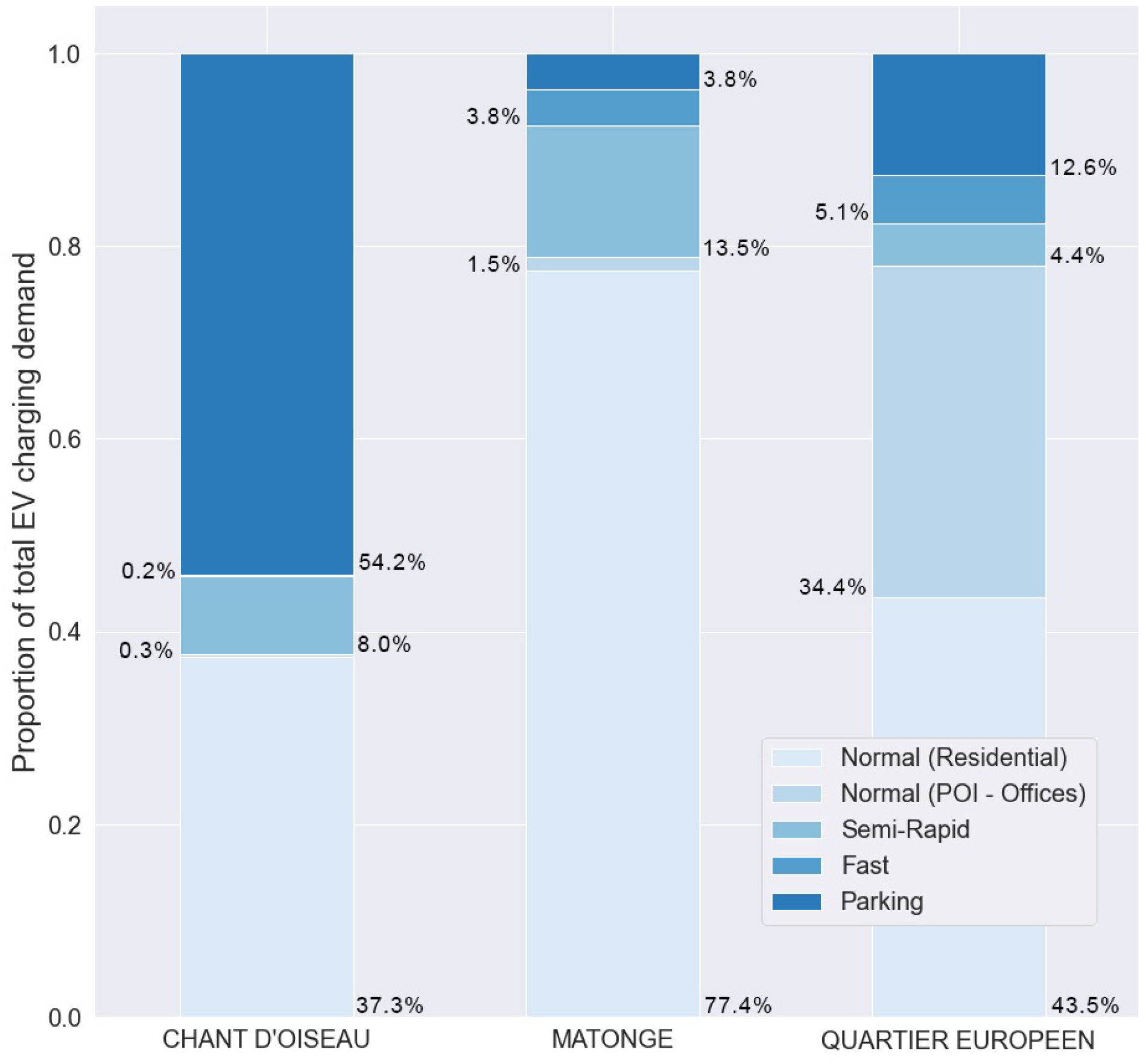
| Neighborhood | Normal (Res) () | Normal (Poi) () | Semi-Rapid () | Rapid () | Parking () |
|---|---|---|---|---|---|
| Chant d’Oiseau | 37.3% | 0.3% | 8.0% | 0.2% | 54.2% |
| Matonge | 77.4% | 1.5% | 13.5% | 3.8% | 3.8% |
| Quartier Européen | 43.5% | 34.4% | 4.4% | 5.1% | 12.6% |
| Charger | Assumption | Value |
|---|---|---|
| Normal | Theoretical Power | 7 kW |
| Avg. Pow. Delivery | 80% | |
| Occupancy Rate | 50% | |
| Opening hours | 24 h/24 h | |
| Semi-Rapid | Theoretical Power | 22 kW |
| Avg. Pow. Delivery | 80% | |
| Occupancy Rate | 80% | |
| Opening hours | 10 h–20 h | |
| Rapid | Theoretical Power | 100 kW |
| Avg. Pow. Delivery | 80% | |
| Occupancy Rate | 25 % | |
| Opening hours | 24 h/24 h |
| Charging Type | Nbr. Stations |
|---|---|
| Normal (Residential) | 11,766 |
| Normal (Work) | 1047 |
| Semi-Rapid | 3004 |
| Rapid | 312 |
| Full Normal | 24,413 |
| Charging Type | Candidate Location |
|---|---|
| Normal (Residential) | On-Street parking, large public parking, etc. |
| Semi-Rapid | Shopping malls, semi-private parking, supermarket parking lots, etc. |
| Rapid | Fuel Stations, intersection of major highways, motorway entrances, etc. |
Disclaimer/Publisher’s Note: The statements, opinions and data contained in all publications are solely those of the individual author(s) and contributor(s) and not of MDPI and/or the editor(s). MDPI and/or the editor(s) disclaim responsibility for any injury to people or property resulting from any ideas, methods, instructions or products referred to in the content. |
© 2023 by the authors. Licensee MDPI, Basel, Switzerland. This article is an open access article distributed under the terms and conditions of the Creative Commons Attribution (CC BY) license (https://creativecommons.org/licenses/by/4.0/).
Share and Cite
Radermecker, V.; Vanhaverbeke, L. Estimation of Public Charging Demand Using Cellphone Data and Points of Interest-Based Segmentation. World Electr. Veh. J. 2023, 14, 35. https://doi.org/10.3390/wevj14020035
Radermecker V, Vanhaverbeke L. Estimation of Public Charging Demand Using Cellphone Data and Points of Interest-Based Segmentation. World Electric Vehicle Journal. 2023; 14(2):35. https://doi.org/10.3390/wevj14020035
Chicago/Turabian StyleRadermecker, Victor, and Lieselot Vanhaverbeke. 2023. "Estimation of Public Charging Demand Using Cellphone Data and Points of Interest-Based Segmentation" World Electric Vehicle Journal 14, no. 2: 35. https://doi.org/10.3390/wevj14020035
APA StyleRadermecker, V., & Vanhaverbeke, L. (2023). Estimation of Public Charging Demand Using Cellphone Data and Points of Interest-Based Segmentation. World Electric Vehicle Journal, 14(2), 35. https://doi.org/10.3390/wevj14020035