Abstract
Intelligent connected vehicles (ICVs) technologies will bring significant changes to future transportation, and urban intersections will be an important scenario for the application of ICVs. There exists one significant challenge to address for the control of ICVs in unsignalized, multi-intersection road networks, that is, how to realize the comprehensive optimization of traffic efficiency and energy saving. To solve this problem, the distributed and hierarchical optimal control architecture is first established in this paper, consisting of a cloud decision layer and a vehicle control layer. For the cloud decision layer, the distributed model predictive control (DMPC) method is utilized for distributed optimization control of multi-intersection road network systems, to achieve optimization in terms of traffic efficiency. For the vehicle control layer, based on the reference speed optimized from the cloud decision layer, the DMPC method is further utilized for distributed optimal control of each vehicle platoon, to achieve optimization in terms of energy saving. Finally, the comparative simulation tests are carried out based on MATLAB and SUMO. The feasibility and effectiveness of the proposed method were verified, and the improvement of traffic efficiency and energy saving was achieved.
1. Introduction
ICVs integrate the advantages of information sharing, advanced sensor technology, and intelligent decision-making technology, which can efficiently exchange information with other ICVs and infrastructure through highly effective communication networks, to realize safe driving for ICVs and improve traffic efficiency at intersections. Compared with one isolated intersection, an unsignalized multi-intersection road network is more complex due to a higher number of intersections and stronger coupling relationship of ICVs’ spatial trajectories in the road segments and intersections [1,2], and in such scenarios, what occurs in an isolated intersection will influence the states of the adjacent intersections and the overall road network. Thus, for urban multi-intersections, the problems of traffic efficiency and fuel consumption are more serious. Therefore, it is of great significance to investigate an optimal control method for ICVs to improve traffic efficiency and energy saving at multi-intersections.
Most studies focus on the cooperative control method of ICVs at one isolated intersection. It mainly uses an intersection management (IM) controller to collect information on the status of all ICVs entering an intersection’s subregions in real time through vehicle-to-infrastructure (V2I) communication and achieve global, multi-objective optimization of the system [2]. Then, the vehicle passing order [3,4], arrival time [5,6,7] or traffic trajectory [8,9,10] can be assigned to each vehicle through V2I communication in real time to realize the cooperative scheduling of ICVs.
However, an urban scenario generally consists of multiple intersections interconnected with each other. In such scenarios, some researchers designed optimization approaches to further improve traffic efficiency at multi-intersections. For example, Wuthishuwong et al. [11,12,13,14] proposed a discrete-time consensus algorithm to balance the traffic flow density of adjacent intersections to improve traffic efficiency. Zhang et al. [15] and Du et al. [16] proposed an optimal control strategy with maximized traffic flow. Pei et al. [17] proposed a distributed strategy to minimize traffic delay for vehicles passing through multi-intersection areas. Doctor et al. [18] presented a sliding mode control with a dynamic boundary method to track congested boundaries and adjust boundary flows according to the state of traffic, to decrease the network’s travel delay. In general, they mainly focused on adjusting the traffic volume from upstream and downstream adjacent intersections to speed up the traffic volume balance, to improve traffic efficiency, but the optimization of ICVs control performances has not yet been considered. To improve the control performance of each ICV, some researchers focused on multi-objective optimization by jointly considering vehicle safety and energy conservation at unsignalized multi-intersections. Zhang et al. [19] presented a decentralized optimal control framework, in which the optimal acceleration/deceleration at any time for each vehicle is obtained, to minimize fuel consumption and ensure driving safety. Wang et al. [20] further proposed a composite strategy for route planning by coordinating the driving speed of ICVs in road networks, to improve vehicle safety and save energy at multi-intersection road networks. Mahbub et al. [21,22] and Zhao et al. [23] formulated a decentralized optimization problem to derive a closed-form analytical solution that yields the optimal control input for each ICV, to decrease fuel consumption. In general, most of the current cooperative control approaches focused on optimizing the ICV control performance by speed harmonization, but the coordination of traffic flow among multi-intersections has not yet been considered.
In summary, the existing research on overall optimization has not yet considered the harmonization of macro-traffic flow density for unsignalized multi-intersection road networks with micro-velocity coordinated control for ICVs. In this paper, we aim to solve the above problems, and the main contributions of this paper are as follows:
(1) A distributed and hierarchical optimal control architecture is developed by considering two layers of optimization objectives: a cloud decision layer and a vehicle control layer. With this architecture, the traffic flow density control (cloud decision layer) and optimal speed control (vehicle control layer) can be organically combined, which makes it possible to achieve a global comprehensive optimization model for traffic efficiency and vehicle control performances at unsignalized multi-intersection road networks.
(2) Different from the existing strategy that only adjusts the traffic flow from adjacent intersections to improve traffic efficiency or only considers multi-objective optimization control for ICVs to improve vehicle control performance, we further extend the results in [16] to propose a multi-objective collaborative optimization control method based on a DMPC algorithm. With this method, the large-scale system with multi-intersection road networks and multi-vehicle groups are decoupled into several intersection subsystems and vehicle subsystems that can interact with each other. On this basis, traffic efficiency and energy consumption are comprehensively considered.
The rest of this paper is organized as follows: Section 2 presents the system architecture. Section 3 presents the DMPC method to realize the comprehensive optimization of traffic efficiency and vehicle consumption at multi-intersection road networks. Numerical experiments are given in Section 4, and we conclude the paper in Section 5.
2. Distributed and Hierarchical Optimal Control Architecture
Benefited from the vehicle-to-vehicle (V2V), V2I, and infrastructure-to-infrastructure (I2I) communications, ICVs can perceive the state of traffic in multi-intersection networks. On this basis, the distributed and hierarchical optimal control architecture is introduced in this paper. By using this architecture, the traffic flow density control (cloud decision layer) and optimal speed control (vehicle control layer) can be organically combined, which makes it possible to realize the global comprehensive optimization of traffic efficiency and energy saving for the ICVs. Moreover, the computational dimension of the optimization problem is also reduced based on the DMPC method for multi-intersection and multi-vehicle systems, which guarantees that a simpler control problem with a lower dimension can be addressed at a time. Figure 1 illustrates the control architecture of this approach consisting of two layers—a cloud decision layer and a vehicle control layer.
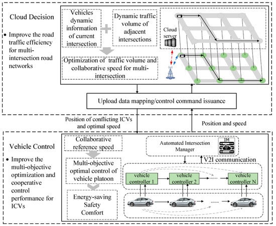
Figure 1.
Distributed and hierarchical optimal control architecture.
For the cloud decision layer, an IM controller is placed at each intersection, to integrate ICVs’ dynamic information entering the current intersection and send the optimized variables and trajectories of conflicts with approaching ICVs, to target ICVs through data mapping upload and control command issuance module. On this basis, we constructed a series of optimization controllers (IM controllers), to improve traffic efficiency based on the DMPC method for multi-intersection road networks. The aim of each optimization controller is to provide optimal reference velocity for ICV controllers and optimal reference traffic flow density for the adjacent IM controllers.
For the vehicle control layer, we designed a distributed controller that focuses on multi-objective control based on the DMPC method according to the optimal reference speed information obtained from upper levels. For each vehicle platoon controller, vehicle safety, energy saving, and passenger comfort were comprehensively considered.
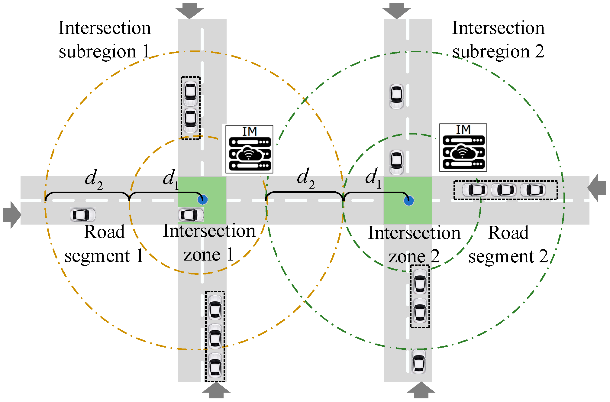
Additionally, since multi-intersection scenario generally consists of multiple intersections interconnected with each other, we divided such scenarios into several intersection subregions. As shown in Figure 2, we took two intersections as an example, and each intersection subregion was divided into two zones, i.e., road segment and intersection zone. In the road segment zone, ICVs were grouped according to driving direction and car-following distance, and then, ICVs had to realize the driving formation of each vehicle platoon according to the optimal reference velocity from the cloud decision layer. In the intersection zone, ICVs adjusted the movement to achieve no-conflict passing at the intersection zone through V2I communication [24]. As the process of dynamic formation is not the focus of this paper, we do not provide a detailed introduction here.
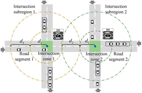
Figure 2.
Studied scenarios of two intersections.
3. Methodology
3.1. Controller Design for Multi-Intersection Road Networks at the Cloud Decision Layer
The DMPC method fully considers the complexity of the whole system with distributed structure, decomposes the large-scale system into several subsystems that can interact with each other, and then transforms the optimization problem into a model solution for each subsystem, which reduces the complexity of the problem and improves the control performance of the system [25]. Additionally, this method was also employed to tackle the uncertainties in the system model [26]. Therefore, an optimal scheduling scheme based on the DMPC method for multi-intersection systems is proposed in this section. This method can improve traffic efficiency through the flexible scheduling of traffic flow and coordination of each adjacent intersection subsystem at multi-intersection road networks.
As shown in Figure 3, we defined a suboptimization predictive problem on each current IM controller (DMPC controller) according to the states of ICVs at current intersections and the traffic states at adjacent intersections. The first optimal control input variable obtained by repeated online optimization is applied to the corresponding ICVs, and the other sequence is transmitted to the adjacent IM controllers through I2I information communications.
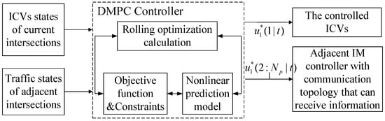
Figure 3.
Control schematic diagram of IM controller based on DMPC method.
Further, it is necessary to solve each single-point model’s predictive optimization problem for all IM controllers at each optimization moment. In the process of distributed model predictive control, the optimal input variables of each IM controller obtained at the last optimization moment was used as the forecasting input at the current moment, and the transfer process of rolling horizon optimization for all IM controllers based on the DMPC algorithm is shown in Figure 4.
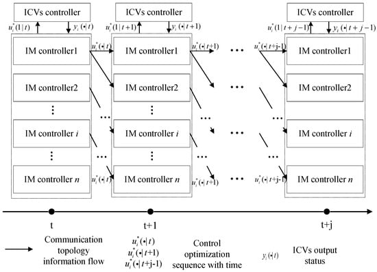
Figure 4.
Flowchart of the DMPC algorithm.
The control goal of the IM controller is to provide optimal speed guidance for ICVs entering the current intersection subregion and to provide predicted information on road traffic flow density for the adjacent IM controllers. We defined the predicted output of the IM controller as , and the expected states of the IM controller as . Additionally, the Greenshield model [16] was used as the prediction model, which provides a simple, linear, functional relationship between average velocity and traffic density. It can be expressed as follows:
where is the road velocity, is the mapping from road density to the road velocity, is the free-flow density, is the free-flow velocity, and is the slope.
In this paper, the cost function can be defined as having two parts: the first is the cost function for traffic efficiency at each intersection, and the second is the cost function of traffic efficiency in the entire road network.
The cost function of traffic efficiency for each intersection is defined as follows:
The first part is to make the predicted states consistent between each road under the control of the IM controller —namely, the states tracking error tend to zero. The second part is to make the predicted states tend toward the desired value, that is, the difference between the current states and the desired states of each road under the control of the IM controller will become smaller and even closer to zero as the control action is applied. It can be expressed as follows:
where is the weighting coefficient of the tracking error between the adjacent IM controllers, and is the weighting coefficient of the tracking error with the desired state. In this paper, the desired road average velocity is calculated to speed up density balancing between road segments, which is similar to [11,12,13,14], and it can be calculated with the following equation:
The cost function of traffic efficiency for the entire road network is defined as follows:
The first part is to make the predicted states between the intersection region and the adjacent region consistent, and the second part is to make the predicted states tend toward the desired value. It can be expressed as follows:
where and , respectively, represent the weighting coefficient.
The optimization problem is described as follows:
Moreover, considering that the traffic system is a real physical system, and in order to ensure the stability of the system, we defined two constraints as follows:
- Speed constraints:
- Traffic flow density constraints:
- where , is the prediction step, represents the maximum road speed, and represents the maximum road density.
3.2. Controller Design for ICVs at the Vehicle Control Layer
The vehicles on the road in a platoon are dynamically decoupled through V2V/V2I communication. Each vehicle node is assigned a local open-loop optimal control problem based on the DMPC algorithm for distributed multi-objective optimization relying on the information from the neighboring nodes and the cloud decision layer.
In this study, we considered the influence of nonlinear characteristics of vehicle dynamics for the approaching ICVs. Additionally, we used nonlinear vehicle longitudinal dynamics models [27] as the prediction models, which are composed of driveline, brake system, aerodynamic drag, tire friction, rolling resistance, and gravitational force, to represent the dynamics of the ICVs. The nonlinear dynamic equation is discretized as follows:
where and are the displacement and velocity of the vehicle , respectively; is the actual driving torque of the vehicle; is the expected driving torque; is the mechanical efficiency of the transmission system; is the delay coefficient of the longitudinal dynamic system; is the mechanical transmission ratio; is the wheel rolling radius; is the air drag coefficient of the vehicle; is the frontal area of the vehicle; is the air density; is the rolling resistance coefficient of the vehicle; is the acceleration of gravity; is the road slope.
In addition, we adopted the fuel consumption model in [28] to calculate the energy consumption of all ICVs; the model is discretized as follows:
where represents the ICVs’ current velocity; , , and are the rolling resistance term and the wind resistance coefficient of the tire; is the mass of the vehicle; is the acceleration of the vehicle; is the engine idle fuel consumption rate; and are the fuel consumption model coefficients.
In this paper, we aimed to design vehicle controllers for a pilot vehicle and the following vehicle, respectively. We assumed that the ego vehicle system output is , . The optimal velocity of the IM controller is , and the corresponding desired location for the vehicle is , so the expected state of the pilot vehicle is . The expected state with regard to the ego vehicle and the pilot vehicle is , where , is the time headway, and is the minimum car-following distance. The expected state of the ego vehicle and the preceding vehicle is , , where .
(1) Objective function and constraints of the pilot vehicle.
The design goal of the pilot vehicle controller is to receive IM controller messages in real time and consider the influence of the upstream and downstream traffic density in multi-intersection road networks on its own torque and driving speed. According to the expected road traffic speed sent by the IM controller, the most economical vehicle torque is calculated and transmitted to the following vehicles. The cost function can be defined in three parts—the first is the tracking error function, the second is the energy-saving function, and the third is the passenger comfort function.
In order to maintain the tracking performance between the cloud control layer and the pilot vehicle, we defined a function that minimizes the tracking error between the desired state of the optimal reference velocity from the IM controller and the actual velocity of the pilot vehicle. Additionally, the tracking error between the expected conflict-free position and actual position also needs to be minimized. The expected conflict-free position can be easily calculated by the minimum safe time headway with the conflict preceding ICVs [19] through the IM controller. ICVs with conflict trajectories can further coordinate the movements of themselves to maintain a safe headway as a result of conflict-free movements, and then, vehicles can pass through the intersection in an orderly manner.
The tracking error cost functions define as follows:
where is the weighting coefficient of the tracking error with the pilot vehicle.
In order to guarantee comfortable ride experiences, we also defined a function to minimize the input torque variation between the predictive control variable and expected control variable, where the desired control variable is obtained from the optimal reference speed of the corresponding IM controller. Therefore, the passenger comfort function is
where is the weighting coefficient of passenger comfort, is the expected torque while the vehicle is driving at the reference speed, and it can be calculated by the following formula: .
The minimum vehicle energy consumption during the predicted time domain is obtained by calculating the minimum vehicle energy consumption accumulated in steps. Therefore, the energy-saving function is
where is the weighting coefficient of energy saving, is the energy consumption function of the pilot vehicle.
The control problem is described as follows:
Additionally, we also designed some constraints as follows:
- Speed constraints: ,
- Acceleration constraints: ,
- Torque constraints: ,
- Speed terminal constraint: ,
- Position terminal constraint: ,
- Torque terminal constraint: ,
- where and , respectively, represent the minimum and maximum speed of the vehicles; and respectively, represent the minimum and maximum acceleration of the vehicles; and , respectively, represent the minimum and maximum torque of the vehicles.
In addition, we designed terminal constraints; for example, the speed of the vehicle at each predicted terminal should be the same as the expected speed; the predicted position should be consistent with the expected position; the vehicle torque needs to be the same as that at the optimum reference speed, to keep the terminal system stable.
(2) Objective function and constraints of the following vehicle.
The design goal of the following vehicle controller is to ensure that its own vehicle runs at the most economical speed while ensuring the safe states of both the car following the pilot vehicle and the preceding vehicle, and establish constraints to ensure the stability of the entire vehicle platoon.
The cost function can also be defined as having three parts—the first is the tracking error function, the second is the comfort function, and the third is the energy-saving function.
The first part is the tracking error between the ego vehicle and the pilot vehicle, while the second part is the tracking error between the ego vehicle and the adjacent vehicles. It is calculated by
where and are the weighting coefficient of the tracking error with the leading vehicle and the adjacent vehicles. and are the position and velocity of the adjacent vehicles.
Passenger comfort and energy-saving functions, respectively, are expressed as follows:
where is the weighting coefficient of comfort, is the weighting coefficient of energy saving, is the energy consumption of each ICV, and is the vehicle torque of the leading vehicle; it can be calculated by the following equation: .
The control problem is described as follows:
There are also some constraints designed as follows:
- Speed constraints:
- Acceleration constraints:
- Torque constraints:
- Speed terminal constraint:
- Position terminal constraint with the preceding vehicle:
- Position terminal constraint with the pilot vehicle:
- Torque terminal constraint:
In the equation, in order to ensure the stability of the vehicle platoon controller, four terminal constraints were also designed. The prediction speed of each prediction terminal needs to be the same as that of the previous vehicle. The predicted position of the ego driving vehicle should be consistent with the expected position of the pilot vehicle and the preceding vehicle. In order to make the terminal system in a stable state, the vehicle torque needs to be consistent with that of the preceding vehicle’s state.
In general, the process of optimization control at the vehicle control layer is similar to the algorithm in the cloud decision layer. We should note that for such a nonlinear constrained optimization-control problem, it is usually necessary to solve the Hamilton–Jacobi–Bellman equation. Since we cannot obtain the analytical solution of the equation, a numerical method is needed for the calculation. The fmincon function in the MATLAB toolbox can calculate iteratively along the descending direction of cost function under the condition of giving initial point and can converge to a locally optimal solution through continuous iterative optimization, so we used this method to solve the constrained nonlinear programming problem.
4. Numerical Experiments
4.1. Scenario Settings and Parameters
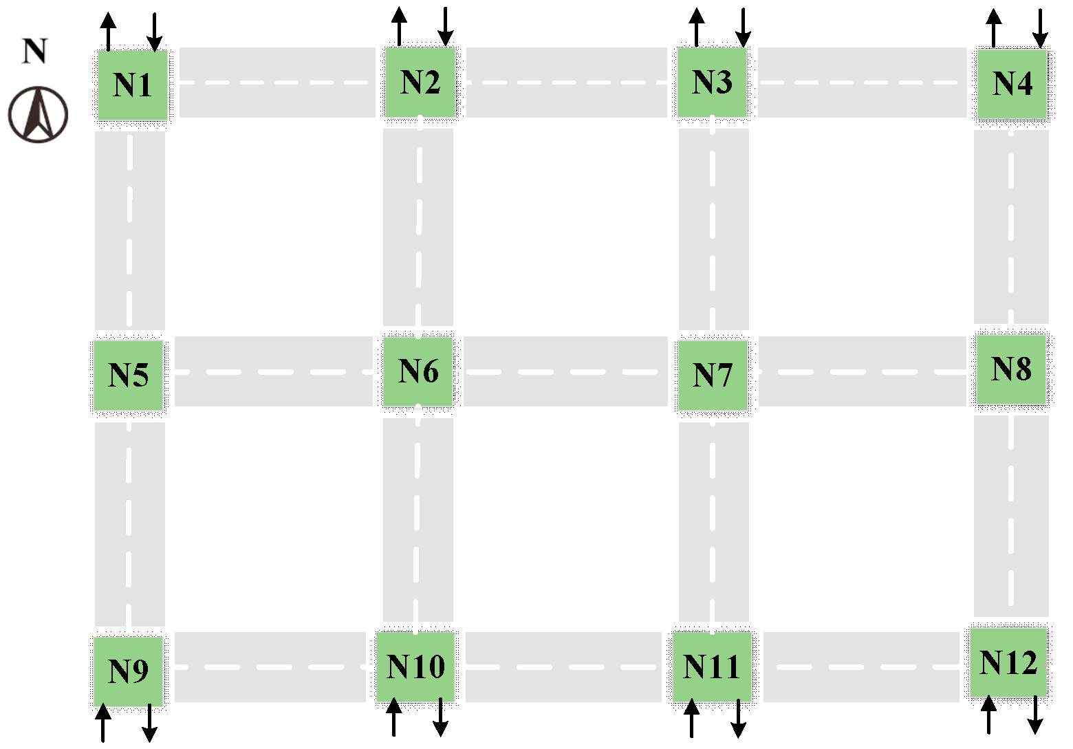
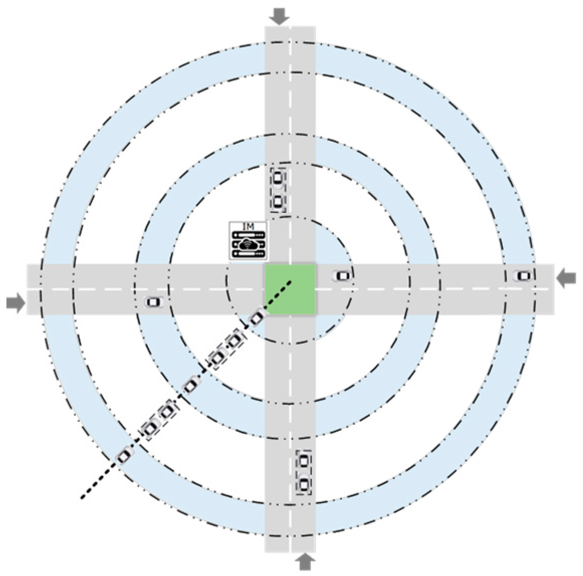
In order to verify the feasibility of the algorithm, in this paper, the joint simulation platform was created by MATLAB and SUMO. Traffic simulation was conducted in SUMO, which is widely used in traffic research [29]. The multi-intersection road networks comprised eight entrances and four intersections (N5–N8), as shown in Figure 5. The distance of adjacent intersections within the control area is 200 m, and the intersection zone is 80 m. In particular, to resolve the trajectories of conflicts with approaching vehicles, such as cross-conflict and confluence conflict at each intersection, as shown in Figure 6, we projected the approaching vehicle platoons from different entrance lanes into virtual lanes according to their location in relation to the intersection origin and constructed a virtual platoon. Further, the conflicting vehicles can coordinate the movements of themselves to pass through the intersection in an orderly manner, while vehicles can realize conflict-free movements.
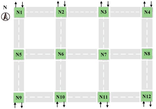
Figure 5.
A schematic diagram of the simulated multi-intersection road networks.
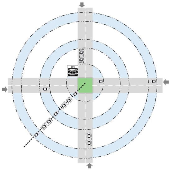
Figure 6.
Virtual platoon projection.
In this paper, the ICVs’ driving direction at each typical intersection was set as follows: 15% of the ICVs go straight, while 10% of the ICVs turn left. In this study, we set the time step as , and the prediction time domain as . The weighting coefficients of the IM controller were, respectively, set as follows: , , , , , and the weighting coefficients of the pilot vehicle controller were, respectively set as follows: , , , and the weighting coefficients of the following vehicle controller in the formation were, respectively, set as follows:, , , . Other key characteristics of the system model are shown in Table 1.

Table 1.
System model characteristics.
4.2. Results
4.2.1. Comparison Tests of Traffic Efficiency and Energy-Saving under Different Traffic Flows
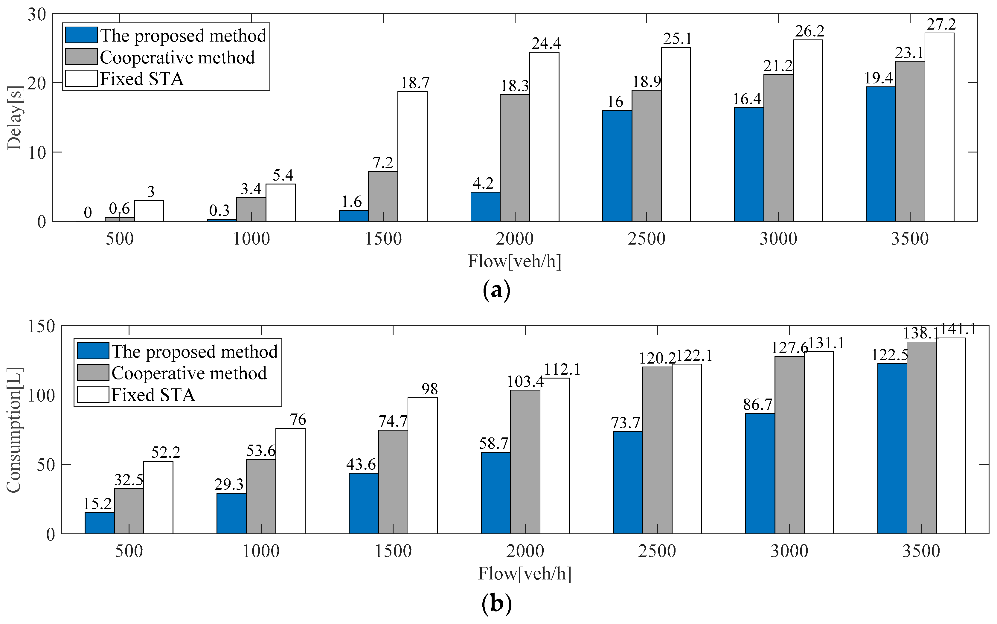
In this scenario, we analyzed the impact of different traffic flows on the performance of the proposed method. The random traffic flow was set from 500 veh/h to 3500 veh/h. Each working condition was simulated 5 times, and simulations ran for 500 steps under different traffic flow conditions. We compared three methods—the proposed method, the cooperative method, and the fixed-signal time assignment (STA) method. In the cooperative method [23], the local IM controller coordinates each vehicle to pass through with a first-in, first-out strategy at each intersection. In addition, there is no coordinated optimization strategy between the adjacent intersection regions as well as no optimization strategy for ICVs. The cycle time of the fixed STA with four phases is 40 s. To verify the effectiveness of the proposed method, the test results of the multi-intersection road networks were calculated. As shown in Figure 7, the comparison results of the delay and consumption with three strategies were calculated using Equations (19) and (20). The improvement effect of the traffic delay and vehicle consumption was calculated with Equation (21).
where represents the intersection regions, and represents the road number in the intersections.
where represents the various flows; represents the delay/consumption of the proposed method under a certain flow; represents the delay/consumption of the benchmark method under a certain flow.
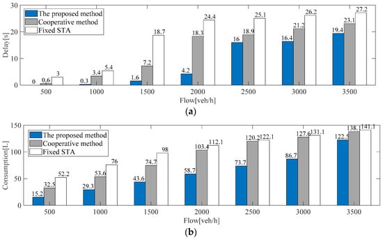
Figure 7.
Comparison results of three methods under different flows: (a) comparison results of delay; (b) comparison results of consumption.
In Figure 7a, compared with the cooperative method, the proposed strategy reduces average delays by about 52.98% on average under different traffic conditions. Compared with fixed STA, the proposed strategy reduces average delays by about 63.13% on average under different traffic conditions. In Figure 7b, compared with the cooperative method, the proposed strategy can reduce fuel consumption by around 37.92% on average in different flows. Compared with the fixed STA method, the proposed strategy can reduce the fuel consumption by about 46.02% on average in different flows. The simulation results illustrate that the proposed method can reduce both traffic delay and fuel consumption of ICVs in multi-intersection road networks.
For the intersection subregions (N5–N8), as can be seen from Figure 8, compared with the benchmark algorithm, the proposed method can also decrease traffic delays and fuel consumption of ICVs under different traffic flow conditions. It may be noted that traffic delay and consumption depend on the traffic flow density of the current intersection subregion as well as the adjacent subregions. Thus, if one subregion has a high traffic delay, and its adjacent subregions have relatively lower delays, the desired velocity for ICVs would be increased according to Equation (7) for the denser subregions, to achieve improvement in road traffic conditions and fuel consumption.
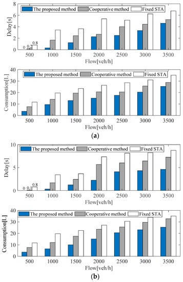

Figure 8.
Comparison results of three methods at intersection subregions under different flows: (a) test results in the intersection subregion N5; (b) test results in the intersection subregion N6; (c) test results in the intersection subregion N7; (d) test results in the intersection subregion N8.
4.2.2. Comparison Tests of Traffic Efficiency and Energy Saving under Sensitivity Analysis
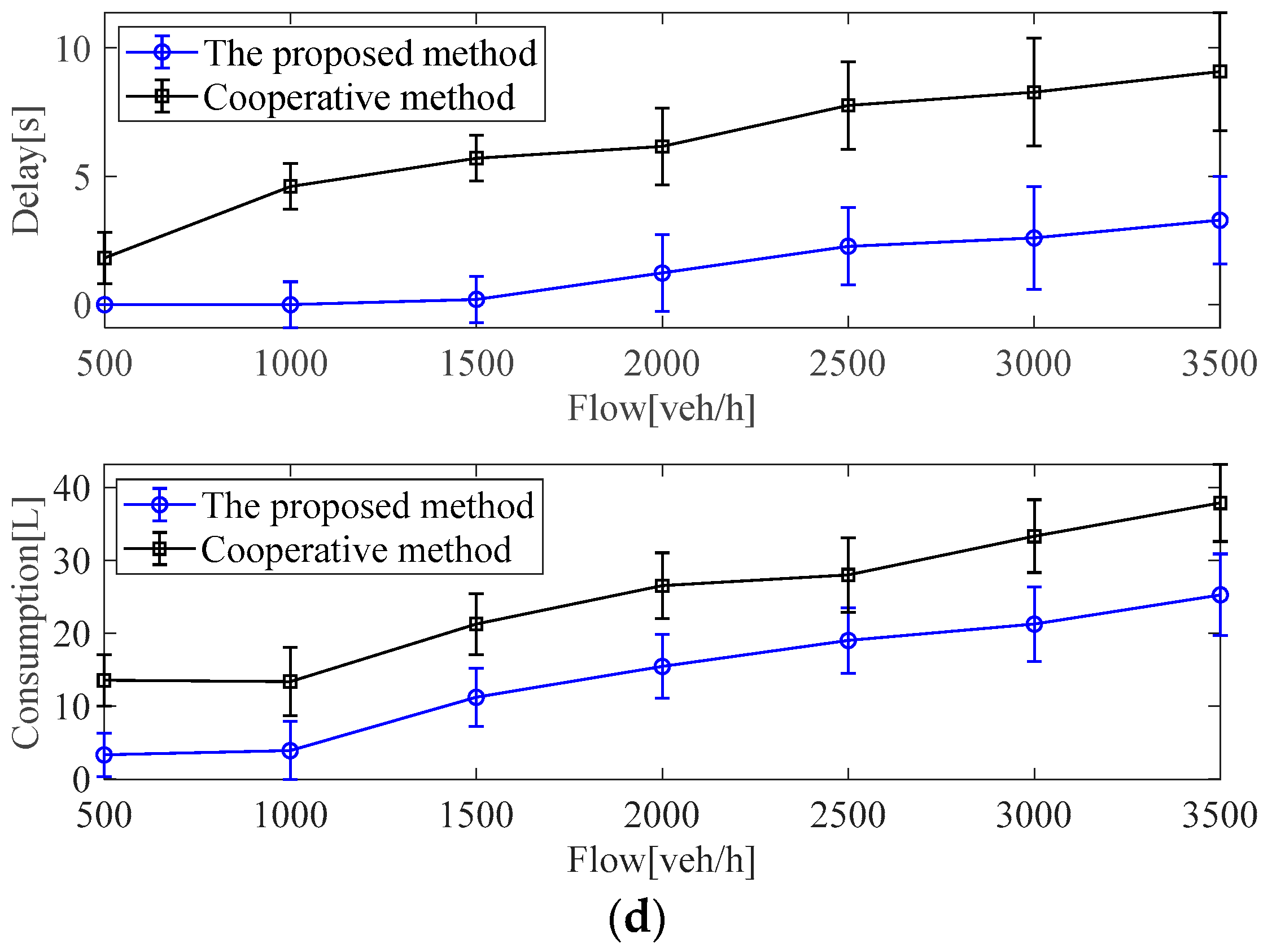
As can be seen from Figure 1, the IM controller can integrate the dynamic position information of ICVs entering the current intersection and regulate the movement of approaching ICVs accurately through V2I communication. However, during this process, the data transmission delay and packet losses between the uplink (status information of ICVs uploaded to the IM controller) and downlink (the control variables from the IM controller downloaded to target ICVs) through V2I communication within a non-ideal communication environment are inevitable. In this scenario, we focused on sensitivity analysis of traffic flow with a time-varying communication time-delay on the control strategy in view of road traffic efficiency and consumption. The random traffic flow was set from 500 veh/h to 3500 veh/h. The tests of traffic delay and fuel consumption under different traffic conditions were uniformly simulated 5 times, and the simulations ran for 500 steps. The bounded time-varying propagation delay of each vehicle satisfied the Rician distribution, as shown in Formula (22), which can reflect the amplitude changes of the transmission signal. To verify the effectiveness of the proposed method, the test results of the multi-intersection road networks were calculated with Equations (19) and (20).
where represents the envelope of sinusoidal (cosine) signal plus narrowband Gaussian random signal, represents the peak value of the main signal amplitude, is the power of the multipath signal component, and , represents a modified Bessel function of order 0 of the first kind, and .
In Figure 9, compared with the cooperative method, the proposed strategy can reduce traffic delays by around 65.56% and can reduce fuel consumption by around 36.02% on average under different traffic flow conditions. The simulation results illustrate that the proposed method can improve the traffic efficiency and fuel consumption of ICVs under different traffic flow conditions with time-varying communication time-delay in multi-intersection road networks.
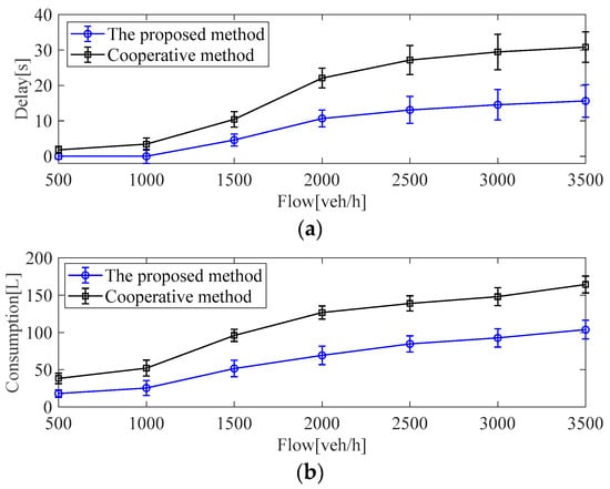
Figure 9.
Test results with two methods under different traffic flow conditions in multi-intersection road networks: (a) comparison results of traffic delay; (b) comparison results of fuel consumption.
For the average delay and consumption in the intersection subregions (N5–N8), as can be seen from Figure 10, compared with the benchmark algorithm in the intersection subregions, the proposed method can decrease the traffic delays and consumption of ICVs under different traffic flow conditions. For benchmark algorithm, due to the time-varying communication time delay, the ICVs cannot track the reference speed sent by the IM controller in time and, thus, cannot realize efficient coordination of the vehicle groups, which causes traffic congestion in the intersection regions, and traffic efficiency and consumption increase rapidly.
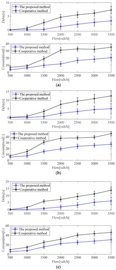
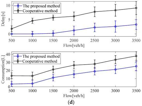
Figure 10.
Test results with two methods under different traffic flow conditions in the intersection subregions: (a) test results in the intersection subregion N5; (b) test results in the intersection subregion N6, (c) Test results in the intersection subregion N7, (d) Test results in the intersection subregion N8.
5. Conclusions
In this paper, a distributed and hierarchical optimal control method was presented to realize the global comprehensive optimization of traffic efficiency and energy saving at unsignalized multi-intersection road networks. With this method, the large-scale system with the multi-intersection road networks and multi-vehicle groups were decoupled into several intersection subsystems and vehicle subsystems that can interact with each other, and thus, a simpler control problem with a lower dimension could be further addressed based on the DMPC method at a time. For the vehicle control layer, the DMPC method was further utilized for a distributed optimal control of each vehicle platoon to achieve the optimization of energy saving based on the reference speed optimized from the cloud decision layer. Simulation results show that, compared with the fixed STA method and the cooperative method, the proposed strategy can, respectively, reduce traffic delays by about 63.13% and 52.98%, and reduce fuel consumption by about 46.02% and 37.92%, respectively, on average, under the different flow conditions, which outperformed the above two baseline methods both in delays and energy consumption. Under the conditions of time-varying communication time delay, compared with the cooperative method, the proposed strategy can reduce delays by around 65.56% and reduce fuel consumption by around 36.02% on average under the different flow conditions, which also outperformed the baseline method in both in delay and energy consumption.
The proposed strategy paves the way for traffic organizers to schedule the movements of large-scale ICVs on a network in real time, to reduce congestion and improve networkwide traffic efficiency, and ICVs can eventually reduce fuel consumption by tracking speed advisory strategies, as well as improving network performance. However, this study did not address traffic problems involving mixed traffic flows in which human-driven vehicles and ICVs share road networks. Our future research extends this approach to mixed traffic scenarios, to provide optimal driving speed reference for human-driven vehicles and ICVs.
Author Contributions
This paper was developed by a research team from the State Key Laboratory of Automotive Safety and Energy. Conceptualization, methodology, and software, J.Y.; formal analysis, investigation, and resources, J.Y. and Y.L.; data curation, J.Y. and Y.L.; writing—original draft preparation, J.Y. and Y.L.; writing—review and editing, J.Y., F.J., Y.L. and W.K.; visualization, J.Y., F.J., Y.L. and W.K.; supervision, F.J. and Y.L. All authors have read and agreed to the published version of the manuscript.
Funding
This study was supported by the independent scientific research project of the State Key Laboratory of Automotive Safety and Energy under Grant ZZ2021-062.
Conflicts of Interest
The authors declare no conflict of interest.
References
- Febbraro, A.D.; Gallo, F.; Giglio, D.; Sacco, N. A traffic management system for smart road networks reserved for self-driving cars. IET Intell. Transp. Syst. 2020, 14, 1013–1024. [Google Scholar] [CrossRef]
- Buzachis, A.; Celesti, A.; Galletta, A.; Fazio, M.; Fortino, G.; Villari, M. A multi-agent autonomous intersection management (MA-AIM) system for smart cities leveraging edge-of-things and Blockchain. Inf. Sci. 2020, 522, 148–163. [Google Scholar] [CrossRef]
- Medina AI, M.; Van De Wouw, N.; Nijmeijer, H. Cooperative intersection control based on virtual platooning. IEEE Trans. Intell. Transp. Syst. 2017, 19, 1727–1740. [Google Scholar] [CrossRef] [Green Version]
- Du, W.; Abbas-Turki, A.; Koukam, A.; Galland, S.; Gechter, F. On the v2x speed synchronization at intersections: Rule based system for extended virtual platooning. Procedia Comput. Sci. 2018, 141, 255–262. [Google Scholar] [CrossRef]
- Yang, K.; Guler, S.I.; Menendez, M. Isolated intersection control for various levels of vehicle technology: Conventional, connected, and automated vehicles. Transp. Res. Part C 2016, 72, 109–129. [Google Scholar] [CrossRef]
- Tallapragada, P.; Cortés, J. Hierarchical-distributed optimized coordination of intersection traffic. IEEE Trans. Intell. Transp. Syst. 2016, 21, 2100–2113. [Google Scholar] [CrossRef]
- Andreas AMalikopoulos Cassandras, C.G.; Yue, J.Z. A decentralized energy-optimal control framework for connected automated vehicles at signal-free intersections. Automatica 2018, 93, 244–256. [Google Scholar]
- Makarem, L.; Gillet, D. Model predictive coordination of autonomous vehicles crossing intersections. In Proceedings of the 16th International IEEE Conference on Intelligent Transportation Systems, The Hague, The Netherlands, 6–9 October 2013; pp. 1799–1804. [Google Scholar]
- Kamal, M.; Imura, J.I.; Hayakawa, T.; Ohata, A.; Aihara, K. A vehicle-intersection coordination scheme for smooth flows of traffic without using traffic lights. IEEE Trans. Intell. Transp. Syst. 2015, 16, 1136–1147. [Google Scholar] [CrossRef]
- Dai, P.; Kai, L.; Zhuge, Q.; Sha, H.M.; Sang, H.S. Quality-of-experience-oriented autonomous intersection control in vehicular networks. IEEE Trans. Intell. Transp. Syst. 2016, 17, 1–12. [Google Scholar] [CrossRef]
- Wuthishuwong, C.; Traechtler, A. Coordination of multiple autonomous intersections by using local neighborhood information. In Proceedings of the International Conference on Connected Vehicles & Expo(ICCVE), Las Vegas, NV, USA, 2–6 December 2013; pp. 48–53. [Google Scholar]
- Wuthishuwong, C.; Traechtler, A. Consensus-based local information coordination for the networked control of the autonomous intersection management. Complex Intell. Syst. 2016, 3, 17–32. [Google Scholar] [CrossRef] [Green Version]
- Wuthishuwong, C.; Traechtler, A. Stability of the consensus in the network of multiple Autonomous Intesections Management. In Proceedings of the International Conference on Automation and Computing (ICAC), Cranfield, UK, 12–13 September 2014; pp. 295–300. [Google Scholar]
- Wuthishuwong, C.; Traechtler, A. Consensus Coordination in the Network of Autonomous Intersection Management. In Proceedings of the International Conference on Informatics in Control, Automation and Robotics (ICINCO), Vienna, Austria, 21–23 July 2015; pp. 794–801. [Google Scholar]
- Zhang, Y.J.; Malikopoulos, A.A.; Cassandras, C.G. Optimal control and coordination of connected and automated vehicles at urban traffic intersections. In Proceedings of the International Conference on American Control Conference (ACC), Boston, MA, USA, 1–3 July 2015; pp. 6227–6232. [Google Scholar]
- Du, Z.; Homchaudhuri, B.; Pisu, P. Hierarchical distributed coordination strategy of connected and automated vehicles at multiple intersections. J. Intell. Transp. Syst. 2018, 22, 144–158. [Google Scholar] [CrossRef]
- Pei, H.; Zhang, Y.; Tao, Q.; Feng, S.; Li, L. Distributed cooperative driving in multi-intersection road networks. IEEE Trans. Veh. Technol. 2021, 70, 5390–5403. [Google Scholar] [CrossRef]
- Ding, H.; Di, Y.; Feng, Z.; Zhang, W.; Zheng, X.; Yang, T. A perimeter control method for a congested urban road network with dynamic and variable ranges. Transp. Res. Part B Methodol. 2022, 155, 160–187. [Google Scholar] [CrossRef]
- Zhang, Y.; Malikopoulos, A.A.; Cassandras, C.G. Decentralized optimal control for connected automated vehicles at intersections including left and right turns. In Proceedings of the International Conference on 2016 IEEE 56th Annual Conference on Decision and Control (CDC), Melbourne, Australia, 12–14 December 2016; pp. 4428–4433. [Google Scholar]
- Mahbub AM, I.; Malikopoulos, A.A.; Zhao, L. Decentralized optimal coordination of connected and automated vehicles for multiple traffic scenarios. Automatica 2020, 117, 108958. [Google Scholar] [CrossRef] [Green Version]
- Mahbub, A.I.; Zhao, L.; Assanis, D.; Malikopoulos, A.A. Energy-optimal coordination of connected and automated vehicles at multiple intersections. In Proceedings of the 2019 American Control Conference (ACC), Philadelphia, PA, USA, 10–12 July 2019; pp. 2664–2669. [Google Scholar]
- Zhao, L.; Malikopoulos, A.A. Decentralized Optimal Control of Connected and Automated Vehicles in a Corridor. In Proceedings of the 2018 IEEE International Conference on Intelligent Transportation Systems (ITSC), Maui, HI, USA, 4–7 November 2018; pp. 1252–1257. [Google Scholar]
- Wang, Y.; Cai, P.; Lu, G. Cooperative autonomous traffic organization method for connected automated vehicles in multi-intersection road networks. Transp. Res. Part C Emerg. Technol. 2020, 111, 458–476. [Google Scholar] [CrossRef]
- Xu, B.; Li, S.E.; Bian, Y.; Li, S.; Ban, X.J.; Wang, J.; Li, K. Distributed conflict-free cooperation for multiple connected vehicles at unsignalized intersections. Transp. Res. Part C Emerg. Technol. 2018, 93, 322–334. [Google Scholar] [CrossRef]
- Parys, R.V.; Pipeleers, G. Distributed mpc for multi-vehicle systems moving in formation. Robot. Auton. Syst. 2017, 97, 144–152. [Google Scholar] [CrossRef]
- Karimi, M.; Roncoli, C.; Alecsandru, C.; Papageorgiou, M. Cooperative merging control via trajectory optimization in mixed vehicular traffic. Transp. Res. Part C Emerg. Technol. 2020, 116, 102663. [Google Scholar] [CrossRef]
- Zheng, Y.; Li, S.E.; Wang, J.; Cao, D.; Li, K. Stability and scalability of homogeneous vehicular platoon: Study on the influence of information flow topologies. IEEE Trans. Intell. Transp. Syst. 2015, 17, 14–26. [Google Scholar] [CrossRef] [Green Version]
- Zhao, W.; Ngoduy, D.; Shepherd, S.; Liu, R.; Papageorgiou, M. A platoon based cooperative eco-driving model for mixed automated and human-driven vehicles at a signalised intersection. Transp. Res. Part C Emerg. Technol. 2018, 95, 802–821. [Google Scholar] [CrossRef] [Green Version]
- Lopez, P.A.; Behrisch, M.; Bieker-Walz, L.; Erdmann, J.; Flötteröd, Y.-P.; Hilbrich, R.; Lücken, L.; Rummel, J.; Wagner, P.; WieBner, E. Microscopic traffic simulation using sumo. In Proceedings of the 2018 21st International Conference on Intelligent Transportation Systems (ITSC), Maui, HI, USA, 4–7 November 2018; pp. 2575–2582. [Google Scholar]


Publisher’s Note: MDPI stays neutral with regard to jurisdictional claims in published maps and institutional affiliations. |
© 2022 by the authors. Licensee MDPI, Basel, Switzerland. This article is an open access article distributed under the terms and conditions of the Creative Commons Attribution (CC BY) license (https://creativecommons.org/licenses/by/4.0/).