Optimal Speed Regulation Control of the Hybrid Dual Clutch Transmission Shift Process ^†

Abstract

This paper presents a gear shift method for the dual clutch transmission (DCT) with integrated electric motor in pure electric drive mode. In contrast to clutch-to-clutch shift in conventional DCT, a good gear shifting process relies on the coordinated control of the motor and synchronizer in electric drive mode of the hybrid DCT. To shorten the torque interruption time and reduce the wear of the synchronizer during engagement, the key point is to adjust the oncoming gear speed to the output shaft speed rapidly. This study provides a speed regulation control framework based on model predictive control (MPC) and disturbance observer (DO), where the MPC controller is designed to achieve a good tracking performance and the DO is to eliminate effects from exogenous disturbances. Simulation and experimental results demonstrate that the proposed approach can attain a rapid and robust gear shifting performance.

1. Introduction

Dual clutch transmission (DCT) has been widely used around conventional vehicle systems because of its advantages in having a simple structure, high efficiency and shifting smoothness. Stringent environmental regulations and fuel consumption limits require more advanced powertrain systems. Electrified DCT has emerged as an applicable technology to electric and hybrid electric vehicle powertrain system [1,2,3,4]. Figure 1 shows the schematic diagram and 3D model of a Motor-Integrated 6-Speed DCT, where the electric motor is coupled onto the shaft with the odd gears (1st, 3rd and 5th) and reverse gear. The hybrid DCT powertrain system provides various driving patterns, including pure electric drive mode, conventional engine drive mode, compound drive mode and regenerative brake mode, meanwhile, the integrated electric motor can also be employed to improve the gear shift quality. Plug-in hybrid electric vehicle equipped with the hybrid DCT will operate in pure electric drive mode until the battery state of charge (SOC) drops to the threshold of charge-sustaining (CS) state. Therefore, to realize a wider range of torque application and higher energy efficiencies than fixed gear ratio, gear shift among the odd gears is necessary. To avoid confusion, the gear shift process discussed in this paper refers to situations when the vehicle is in pure electric drive mode. In this circumstance, the hybrid DCT can be seen as a clutchless automatic manual transmission (CLAMT). Previous research on the CLAMT system can inspire developing an improved gear shift control strategy in the hybrid DCT. Unlike the clutch-to-clutch shift method applied in conventional DCT, a good gear shift process of the CLAMT system relies on the coordinated control of the motor and synchronizer. Regardless of the specifics of these gear shift methods, it is critical that the speed of the oncoming gear can be adjusted to that of the output shaft rapidly and smoothly.

Liu et al. introduced a CLAMT powertrain system in an electric bus, where the clutch and synchronizer within the traditional automatic manual transmission (AMT) are both omitted. Since there are no friction elements, to abate “kick tooth” phenomenon, the electric motor must have a high-precise speed adjustment ability to make the speed completely equal between two engaging elements [5]. However, the abolition of clutch and synchronizer makes the function of mode transition and gear preselection impossible. Tseng et al. parsed out the process of the CLAMT gear change into several phases: gear release, gear select, motor speed regulation (electronic synchronization), gear engagement (mechanical synchronization) and torque recover. This study demonstrated that the precision of the motor speed adjustment can highly affect the subsequent gear engagement phase. The electronic synchronization phase accounts for nearly 65% of the total gear shift time in some cases [6]. Walker et al. proposed a common proportional-integral-derivative (PID) controller to enable closed-loop speed control for motor speed synchronization [7]. To reduce the time of speed adjustment, some advanced control strategies have already been adopted. The fixed-gain PID controller can be replaced by a sliding mode controller (SMC) [8]. Zhu et al. designed a robust speed synchronization control scheme which combined preview control, integral control and state-feedback control together. By employing the H${}_{\infty }$ performance index for investigating and optimizing the controller, the controller design problem is transformed into a linear matrix inequality (LMI) problem [9]. The CLAMT systems in the above study are all applied in electric vehicles, so the transient speed regulation phase is achieved by the electric motor. Some researchers have discussed the possibility of canceling the clutch in the traditional automatic manual transmission (AMT) car. Zhong et al. utilized a combined control algorithm based on feed-forward, bang-bang and PID control for an accurate engine speed control in a conventional AMT [10]. In a vehicle Controller Area Network (CAN) based control system, the network-induced delays can lead to an oscillation phenomenon in the speed regulation phase of gear shift. To guarantee the robustness of the speed regulation controller, various methods, such as energy-to-peak performance-based control and an active period-scheduling approach, are presented [11,12,13]. Overall, whether used in conventional vehicles or hybrid electric vehicles, these studies on CLAMT powertrain control highlight the significance of realizing a rapid and robust motor speed synchronization process.

It is worth noting that the gear shift process of the hybrid DCT shown in Figure 1 confronts some other challenges. A big gear ratio difference between adjacent odd gears and large inertia to be synchronized may consume more gear shift time. Due to the cooling and lubrication requirements, the motor rotor within the hybrid DCT gearbox is cooled by automatic transmission fluid (ATF). As a result, the motor output torque may be disturbed by oil stirring resistance during gear change [14]. For the problem of unknown disturbance torque in the motor speed synchronization process, the common practice is to integrate robust controller designs, like H${}_{\infty }$ control scheme [9,15,16], sliding mode control (SMC) [12,17,18]. However, H${}_{\infty }$ control needs to make a tradeoff between robustness and transient responses and may be over-conservative. As for SMC, it tends to cause chattering and a boundary layer is usually needed, which can deteriorate its capability of disturbances rejection.

In this paper, a combined speed regulation controller for the hybrid DCT is proposed. The model predictive control (MPC) controller is adopted to ensure good tracking performance and the disturbance observer (DO) is applied to improve the robustness of the transient performance. The rest of the paper is organized as follows. In Section 2, the gear shift process of the hybrid DCT and the powertrain mathematical modeling are introduced. Section 3 presents the designed gear shift method. Section 4 shows the simulation and experiment results. Conclusions are drawn in Section 5.

2. Problem Formulation

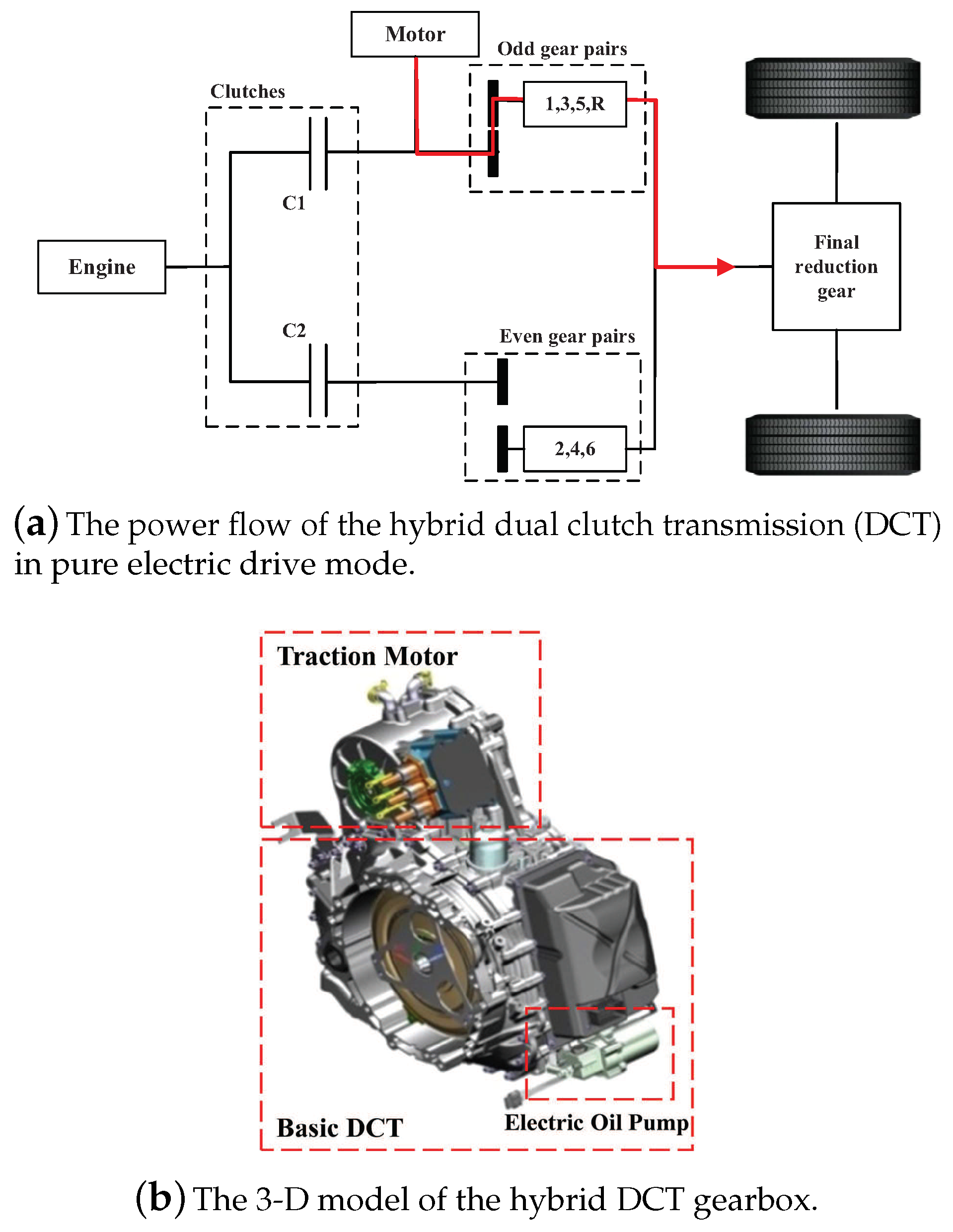
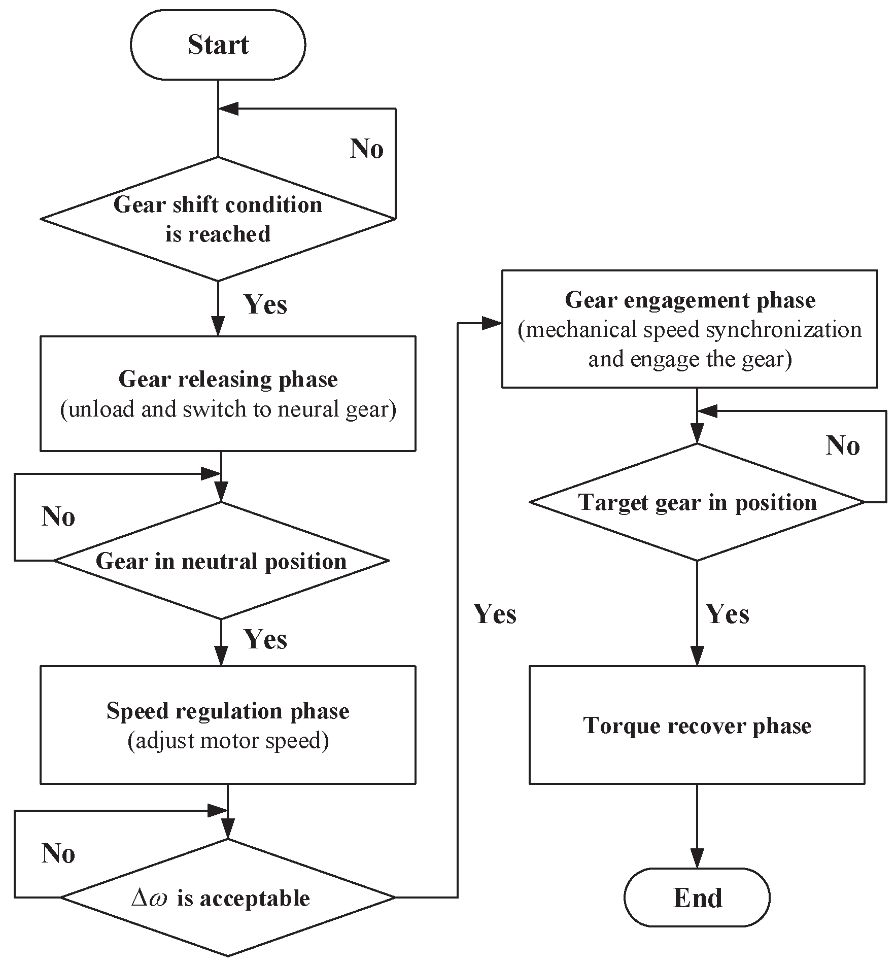
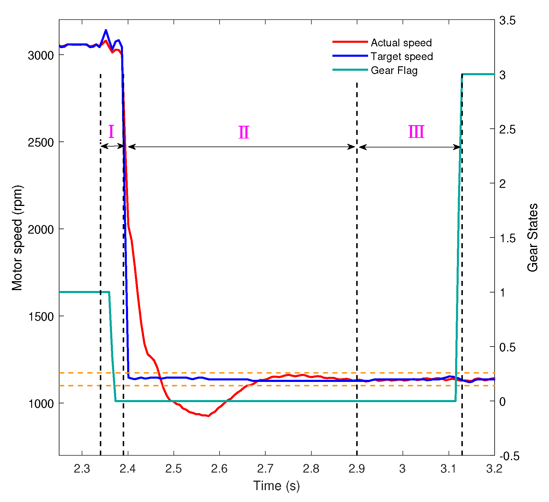
2.1. Gear Shift Process in Pure Electric Drive Mode

The structural details and electrical connections of the hybrid DCT powertrain system are depicted in Figure 2. The CAN bus allows to exchange measurement and control signals among controller units. Vehicle control unit (VCU) provides an overarching control of the hybrid powertrain system and it coordinates the work between other controller units such as Motor control unit (MCU), Transmission control unit (TCU), Battery management system (BMS) and Engine control unit (ECU) during mode transition and gear shift process.

Figure 3 shows the flowchart of the gear shift process. VCU will determine whether a gear shift event is activated based on gear shift schedule and send the gearshift request signal to MCU and TCU once the gear shift condition is met. Then MCU controls the motor to unload quickly and sends the motor output torque signal through CAN in real time. When TCU detects that the motor output torque is reduced to zero, it can manipulate the shift force control solenoid to disengage synchronizer from the current engaged gear.

The gear shift process can forward to the speed regulation phase if the synchronizer is totally released. The motor control unit (MCU) will adjust the motor speed to the target value according to the proposed algorithm deployed in the vehicle control unit (VCU). The process of the speed adjustment will last until the speed difference is within an acceptable range. The chosen threshold depends on the mechanical characteristics of the gears and synchronizers and can be determined by synchronizer bench test [5]. The transmission control unit (TCU) will drive the synchronizer to engage the oncoming gear after the motor speed is stabilized around the target speed for a certain time. The synchronizer can generate friction torque to make the speed of the two engaging elements completely equal. Since the motor speed has been very close to the target speed after the speed regulation phase, the wear and tear of the gears and synchronizers during engagement will be substantially reduced. After the gear engagement phase is finished, MCU will response to the torque request signal from VCU on the basis of energy management strategy.

2.2. Powertrain Model and Parameters Identification

This paper mainly concerns with how to reduce the speed regulation time while ensuring a smooth gear engagement process by suppressing the motor speed and torque fluctuation before engagement. Since the clutches and synchronizers are fully disengaged in speed regulation phase, the dynamic model of the hybrid DCT powertrain system is degenerated into a 2-DOF model. The equations of the system are as follows:

$$J_{e,m}{\dot{\omega }}_m=T_m-b_{e,m}{\omega }_m-T_f$$

(1)

$$J_v{\dot{\omega }}_v=-(Mgrsin\theta +\frac{1}{2}{\rho }_{air}A{C}_D{V}^{2}r+Mgfrcos\theta ),$$

(2)

where ${\omega }_m$ and ${\omega }_v$ are the rotational speed of the motor and wheel, r is the radius of the tire, $J_v$ is the vehicle inertia, $b_{e,m}$ is the lumped viscous damping coefficient at the motor output shaft, $T_f$ can be treated as an unknown disturbance torque, $T_m$ is the motor output torque. The right three parts of Equation (2) are known as incline resistance, aerodynamic resistance and rolling resistance, where M is vehicle mass, g is gravity, $\theta$ is incline angle, ${\rho }_{air}$ is air density, A is vehicle frontal area, $C_D$ is drag coefficient, V is vehicle velocity and f is the rolling resistance coefficient. It should be noted that $J_{e,m}$ denotes the equivalent inertia converted to the motor output shaft such as clutch driven plates, solid primary shaft, motor rotor and shaft, the gears which are rigidly connected to the shaft.

The aim of the speed regulation phase is to adjust the motor speed ${\omega }_m$ to the target speed ${\omega }_m^{Tg}$. The target speed of the motor can be calculated as:

$${\omega }_m^{Tg}={\omega }_v·i_{g,NG},NG=1,3,5,$$

(3)

where $i_{g,NG}$ is the ratio of the oncoming gear. Because the vehicle inertia is comparatively large and there is no power output during gear shift process, the vehicle speed is assumed to be constant. It is obviously that the motor speed should decrease to the target speed in upshift scenario and increase to that in downshift process. According to the analysis of the preceding gear shift process, the speed regulation phase control can be simplified as a tracking problem, where the reference trajectory can be obtained from Equation (3).

The effectiveness of the controller depends to a great extent on the accuracy of the controlled model. The dynamic characteristics of the motor shaft during the speed regulation process are mainly determined by parameters like $J_{e,m}$ and $b_{e,m}$. These parameters need to be identified off-line from experimental data. The test scenarios are as follows: The hybrid DCT powertrain is in neutral gear and MCU receives a constant motor command from VCU. Once the motor is driven to a certain speed, MCU controls the motor to be de-energized. For example, in test case 1, the motor is driven to about ${\omega }_m=3000$ rpm by a constant positive torque command $T_m=4$ Nm and then shut off. The motor torque command and the ramp up and down of the actual speed trajectory are used as input and output for identification in System Identification Toolbox of MATLAB/Simulink.

Figure 4 shows that the simulated outputs using the identified parameters can be well matched with the measured outputs, which demonstrates a good accuracy of the identification of the model parameters. However, it can be seen that there are still some deviations exist even in the case of a quite small output torque. Under real speed synchronization circumstance, a large speed adjustment in a short time needs a big and time-varying motor torque command, which may result in worse response. Therefore, a robust controller against disturbance is necessary.

The identified and default parameters of the powertrain system are listed in

Table 1. Main parameters used in controller design.

Symbol	Variable Name	Value	Unit
$J_{e,m}$	Equivalent inertia of the motor shaft	0.0192	$\mathrm{kg}·{\mathrm{m}}^2$
$b_{e,m}$	Lumped viscous damping coefficient	0.0011	$\mathrm{Nm}·\mathrm{s}/\mathrm{rad}$
$i_{g,1}$	First gear ratio (reduction gear included)	27.086	/
$i_{g,3}$	Second gear ratio	10.318	/
$i_{g,5}$	Third gear ratio	5.872	/

.

3. Controller Design

To ensure smooth gear engagement in the following phase, a combined speed regulation controller of the motor speed adjustment is introduced. The overall control scheme is illustrated in Figure 5. The MPC controller is adopted to achieve a good tracking performance. The predicted behavior is taken into account, thus not only the current tracking error can be suppressed but also the future errors [19]. Considering that the model parameters’ error or external disturbances exist, a discrete-time DO is combined to enhance the robustness of the nominal controller.

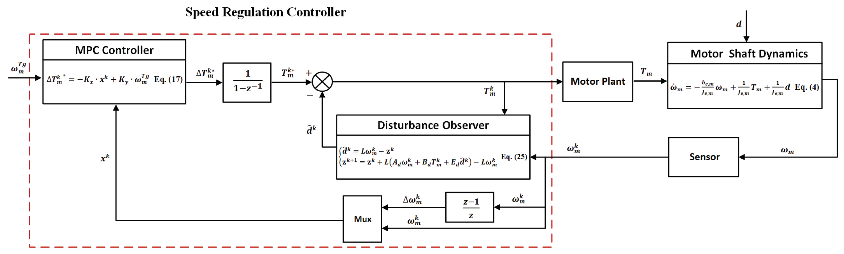
3.1. MPC Controller Design

According to Equation (1), the motor shaft dynamics can be represented as:

$${\dot{\omega }}_m=-\frac{b_{e,m}}{J_{e,m}}{\omega }_m+\frac{1}{J_{e,m}}{T}_m+\frac{1}{J_{e,m}}d,$$

(4)

where d denotes the lumped disturbance torque acting on the motor output shaft. In automotive applications, it is convenient to represent the system in discrete-time form via:

$${\omega }_m^{k+1}=A_d{\omega }_m^k+B_d{T}_m^k+E_d{d}^k,$$

(5)

where the coefficients $A_d$, $B_d$ and $E_d$ can be obtained by discretizing the Equation (4) using Zero-order hold. The superscript k is a nonnegative integer denoting the sample number which is connected to time by $t=k·T$. The sampling time T is chosen the same as the sampling period of the speed sensor in real experiment.

Assuming that the disturbance torque is an unknown constant, d can be removed from Equation (5) with the incremental modelling technique [20]. As for the more complicated case where d is not a constant, we will consider it in the following DO design part. The incremental form of Equation (5) can be derived by taking a differential operation on both sides, such as $\Delta {\omega }_m^{k+1}={\omega }_m^{k+1}-{\omega }_m^k$.

$$\Delta {\omega }_m^{k+1}=A_d\Delta {\omega }_m^k+B_d\Delta T_m^k.$$

(6)

The augmented state space model for the controller design can be expressed as Equation (7).

$$\stackrel{x^{k+1}}{\overbrace{\left[\begin{array}{c}\Delta {\omega }_m^{k+1}\\ {\omega }_m^{k+1}\end{array}\right]}}=\tilde{A}\stackrel{x^k}{\overbrace{\left[\begin{array}{c}\Delta {\omega }_m^k\\ {\omega }_m^k\end{array}\right]}}+\tilde{B}\stackrel{\Delta u^k}{\overbrace{\Delta T_m^k}}$$

(7)

$$y^k=\tilde{C}\left[\begin{array}{c}\Delta {\omega }_m^k\\ {\omega }_m^k\end{array}\right].$$

(8)

The state variable is chosen to be $x^k={[\Delta {\omega }_m^k,{\omega }_m^k]}^T$ and the coefficient matrices of the state space equations are given as Equation (9).

$$\tilde{A}=\left[\begin{array}{cc}{A}_d& 0\\ A_d& 1\end{array}\right],\tilde{B}=\left[\begin{array}{c}{B}_d\\ B_d\end{array}\right],\tilde{C}=\left[\begin{array}{cc}0& 1\end{array}\right].$$

(9)

Let M and P denote the control horizon and prediction horizon, respectively. Note that the control variable $T_m^k$ remains unchange outside the control horizon, the recursive relation of state vectors can be derived from Equation (10).

$$x^{k+i|k}={\tilde{A}}^i{x}^k+\sum _{l=0}^{i-1}{\tilde{A}}^l\tilde{B}\Delta u^{k+i-l-1},i=1,\cdots ,P,$$

(10)

where $x^{k+i|k}$ denotes the predicted state variable at sample instant $k+i$ with initial state $x^k$. Substituting Equation (10) into Equation (8), the output sequences can be obtained as:

$$Y_P=S_x{x}^k+S_u\Delta {\mathrm{U}}_M$$

(11)

with

$$Y_P\triangleq \left[\begin{array}{c}{y}^{k+1|k}\\ ⋮\\ y^{k+P|k}\end{array}\right]=\left[\begin{array}{c}{\omega }_m^{k+1|k}\\ ⋮\\ {\omega }_m^{k+P|k}\end{array}\right],\Delta {\mathrm{U}}_m\triangleq \left[\begin{array}{c}\Delta u^k\\ ⋮\\ \Delta u^{k+M-1}\end{array}\right]=\left[\begin{array}{c}\Delta T_m^k\\ ⋮\\ \Delta T_m^{k+M-1}\end{array}\right]$$

(12)

and

$$S_x=\left[\begin{array}{c}\tilde{C}\\ ⋮\\ \tilde{C}{\tilde{A}}^M\\ ⋮\\ \tilde{C}{\tilde{A}}^P\end{array}\right],S_u=\left[\begin{array}{ccc}\tilde{C}\tilde{B}& \cdots & 0\\ ⋮& \ddots & ⋮\\ \tilde{C}{\tilde{A}}^{M-1}\tilde{B}& \cdots & \tilde{C}\tilde{B}\\ ⋮& \ddots & ⋮\\ \tilde{C}{\tilde{A}}^{P-1}\tilde{B}& \cdots & \tilde{C}{\tilde{A}}^{P-M}\tilde{B}\end{array}\right].$$

(13)

The speed regulation phase control is simplified as a tracking problem, where the reference trajectory is obtained from Equation (3). The optimal control problem is to adjust the motor speed to its target value, then the cost function of the prediction horizon can be defined as:

$$\begin{array}{cc}\hfill J& =\sum _{i=1}^P{\Gamma }_{q,i}·\parallel {\omega }_m^{k+i|k}-{\omega }_m^{Tg}{\parallel }^2+\sum _{i=1}^M{\Gamma }_{r,i}·{\parallel \Delta T_m^{k+i-1}\parallel }^2\hfill \\ \hfill & ={(W_P-Y_P)}^{T}Q(W_P-Y_P)+\Delta {\mathrm{U}}_M^{T}R\Delta {\mathrm{U}}_M^T,\hfill \end{array}$$

(14)

with $W_P=[{\omega }_m^{Tg},\cdots ,{\omega }_m^{Tg}]$, $Q\triangleq diag({\Gamma }_{q,1},\cdots ,{\Gamma }_{q,P})$ and $R\triangleq diag({\Gamma }_{r,1},\cdots ,{\Gamma }_{r,M})$.

In Equation (14), Q is the weighting matrix to penalize track errors and is chosen to be real symmetric and positive semi-definite, while R is related to the control action and can be regarded as a soft constraint imposed on control variable. Notice that the cost function depends on the initial state $x^k$ and input sequences $\Delta {\mathrm{U}}_M$, the optimal solution can be formulated as follows:

$$\Delta {\mathrm{U}}_M^{*}=arg\underset{\Delta {\mathrm{U}}_M}{min}J(x^k,\Delta {\mathrm{U}}_M).$$

(15)

Based on convex optimization theory [17], in the absence of constraints, Equation (15) can be solved as:

$$\Delta {\mathrm{U}}_M^{*}={(S_u^{T}Q{S}_u+R)}^{-1}{S}_u^{T}Q(W_P-S_x{x}^k).$$

(16)

The moving horizon control law uses the first move of the optimal control sequence, that is, the optimal control at step k is

$$\begin{array}{cc}\hfill \Delta T_m^{k*}& =-K_x·x^k+K_y·{\omega }_m^{Tg}\hfill \\ \hfill & =-K_x·\left[\begin{array}{c}\Delta {\omega }_m^k\\ {\omega }_m^k\end{array}\right]+K_y·{\omega }_m^{Tg}\hfill \end{array}$$

(17)

with

$$\begin{array}{cc}\hfill K_x& =\left[\begin{array}{ccc}1& \cdots & 0\end{array}\right]{(S_u^{T}Q{S}_u+R)}^{-1}{S}_u^{T}Q{S}_x\hfill \\ \hfill K_y& =\left[\begin{array}{ccc}1& \cdots & 0\end{array}\right]{(S_u^{T}Q{S}_u+R)}^{-1}{S}_u^{T}Q\left[\begin{array}{c}1\\ ⋮\\ 1\end{array}\right].\hfill \end{array}$$

(18)

Equation (17) gives a feedforward-feedback control law. If the weighting matrices are determined, the gain matrices can be precomputed off-line and the control action applied to the plant can be obtained on-line.

3.2. Controller Parameters Tuning

According to Equation (14), MPC inherits the tuning challenge of the weighting matrices of linear quadratic regulator (LQR) control. The tuning parameters of the MPC controller consist of control horizon, prediction horizon and weighting matrices. Each of the above parameters has a specific role in system performance and it is not always obvious to select an appropriate value.

Substituting Equation (17) into Equation (7), the closed-loop controlled system of the speed regulation phase can be represented as:

$$x^{k+1}=(\tilde{A}-\tilde{B}{K}_x)x^k+\tilde{B}{K}_y{\omega }_m^{Tg}.$$

(19)

Since the Equation (19) represents a second-order discrete-time system, a quantitative relationship between the closed-loop performance and the tuning parameters can be obtained. The dynamic performance of a second-order continuous system $G\left(s\right)={\omega }_n^2/(s^2+2\zeta s+{\omega }_n^2)$ can be characterized by the maximum overshoot $\delta$ and settling time $t_s$ in engineering practice. Given the maximum overshoot and the settling time requirements, the desired closed-loop poles $p_{det}$ of the equivalent discrete-time transfer function $G\left(z^{-1}\right)$ can be determined.

The gain matrix $K_x$ satisfying the specified pole locations can be derived from Ackermann Formula [21]. As for the feedforward gain matrix $K_y$, according to Equations (8) and (19), it can be derived as follows:

$$K_y=\frac{y^{k+i|k}-\tilde{C}{(\tilde{A}-\tilde{B}{K}_x)}^i{x}^k}{\tilde{C}{\sum }_{l=0}^{i-1}{(\tilde{A}-\tilde{B}{K}_x)}^l\tilde{B}{\omega }_m^{Tg}},i=1,\cdots ,\infty .$$

(20)

Since the stability of the closed-loop system represented by Equation (19) is guaranteed by the eigenvalues of $\tilde{A}-\tilde{B}{K}_x$, then $\tilde{C}{(\tilde{A}-\tilde{B}{K}_x)}^i{x}^k\to 0$ as $i\to \infty$. Moreover, the track error $y^{k+n|k}-{\omega }_m^{Tg}$ converges to zero. Equation (20) can be simplified as:

$$K_y=\underset{i\to \infty }{lim}\frac{1}{\tilde{C}{\sum }_{l=0}^{i-1}{(\tilde{A}-\tilde{B}{K}_x)}^l\tilde{B}}.$$

(21)

It should be noted that i must be large enough to ensure a zero offset. Equation (21) indicates that $K_y$ can be calculated with system matrices and gain matrix $K_x$. However, it involves with computing the powers of matrix. In this paper, $K_y$ can be directly given by the last columns of the gain matrix $K_x$ due to the specific form of state transition matrix and output matrix in Equation (8).

Revisiting Equation (18), it is clear that the gain matrices can be obtained once the weighting matrices are determined and vice versa. The above steps give the gain matrices with the specified closed-loop pole locations $p_{det}$, then Q and R need to satisfy the following equation:

$$\left[\begin{array}{ccc}1& \cdots & 0\end{array}\right]{(S_u^{T}Q{S}_u+R)}^{-1}{S}_u^{T}Q{S}_x-K_x=0.$$

(22)

Considering the unknowns ${\Gamma }_{r,1},\cdots ,{\Gamma }_{r,M}$ and ${\Gamma }_{q,1},\cdots ,{\Gamma }_{q,P}$, the Equation (22) can be rewritten as:

$$f_i({\Gamma }_{r,1},\cdots ,{\Gamma }_{r,M},{\Gamma }_{q,1},\cdots ,{\Gamma }_{q,P})=0,i=1,2.$$

(23)

The number of unknowns of Equation (23) depends on the size of the control horizon M and prediction horizon P. The linear equality constraints shown in Equation (23) may be too strict to be solved exactly when the size of the control and prediction horizon increase. Thus the relaxation variables ${\alpha }_1$ and ${\alpha }_2$ are introduced to construct a linear programming (LP) problem shown in Equation (24). The linear equality constraints are relaxed into inequality constraints in the following optimization problem. Then the numerical solution can be obtained in the framework of convex optimization. When the feasible solution of the optimization problem (24) makes the relaxation variable get a very small value, it is equivalent that the solutions has returned near-optimal weight matrices Q and R which achieve the corresponding $K_x$.

$$\begin{array}{cc}\hfill \underset{Q,R,\alpha }{min}& {\alpha }_1+{\alpha }_2\hfill \\ \hfill \mathrm{s}.\mathrm{t}.& -{\alpha }_i\le f_i({\Gamma }_{r,1},\cdots ,{\Gamma }_{r,M},{\Gamma }_{q,1},\cdots ,{\Gamma }_{q,P})\le {\alpha }_i,\hfill & \hfill & i=1,2\hfill \\ \hfill & Q\succ 0,R⪰0,\hfill \\ \hfill & {\alpha }_i\ge 0.\hfill \end{array}$$

(24)

Equation (24) is a typical constrained optimization problem and there are some general solutions to the above optimization problem, such as the simplex method and the interior-point method. In this paper, the interior-point algorithm is chosen to solve the LP problem. For further details of solving the constrained optimization problem, refer to Wright and Nocedal’s book [22].

3.3. Disturbance Observer Design

The incremental form MPC design can suppress the unknown constant disturbance but it is useless against a periodic and random perturbation. In practice, parameters mismatch can also degenerate control performance, sometimes it may cause unstable and oscillation. To solve the problem, a discrete-time disturbance observer for Equation (5) is introduced as:

$$\left\{\begin{array}{cc}\hfill {\widehat{d}}^k& =L{\omega }_m^k-z^k\hfill \\ \hfill z^{k+1}& =z^k+L(A_d{\omega }_m^k+B_d{T}_m^k+E_d{\widehat{d}}^k)-L{\omega }_m^k,\hfill \end{array}\right.$$

(25)

where ${\widehat{d}}^k$ is the estimation of the disturbance, $z^k$ is an intermediate variable, L is the observer gain and can be tuned to satisfy different estimation demands.

Contrary to the hypothesis that the disturbance is constant in the MPC controller design part, the disturbance is assumed to be slowly time-varying in actual speed synchronization circumstance, that is, $|\Delta d^k|\le \epsilon$, $\forall k=1,\cdots ,\infty$, $\epsilon ϵN$.

The disturbance estimate error is defined as $e_{d^k}\triangleq d^k-{\widehat{d}}^k$. From Equations (5) and (25), the recursive relation of the estimate error can be derived as:

$$e_{d^{k+1}}=(I-L{E}_d)e_{d^k}+\Delta d^{k+1}.$$

(26)

Equation (26) is asymptotically stable if the eigenvalues of $I-L{E}_d$ are less than unity, which means the estimate error converges to a bound as T increases.

$$\begin{array}{cc}\hfill \underset{n\to \infty }{\underbrace{|e_{d^{k+n}}|}}& =\underset{n\to \infty }{lim}|{(I-L{E}_d)}^n{e}_{d^k}+\sum _{i=1}^{n-1}{(I-L{E}_d)}^{i-1}\Delta d^{k+1}|\hfill \\ \hfill & \le \underset{n\to \infty }{lim}\sum _{i=1}^{n-1}{(I-L{E}_d)}^{i-1}\epsilon \simeq \frac{\epsilon }{L{E}_d}.\hfill \end{array}$$

(27)

Since Equation (5) is a scalar equation, the observer gain should satisfy the following equation and the value of L can be tuned for a robustness or aggressive estimate speed.

$$0\le L\le \frac{2}{E_d}.$$

(28)

4. Results

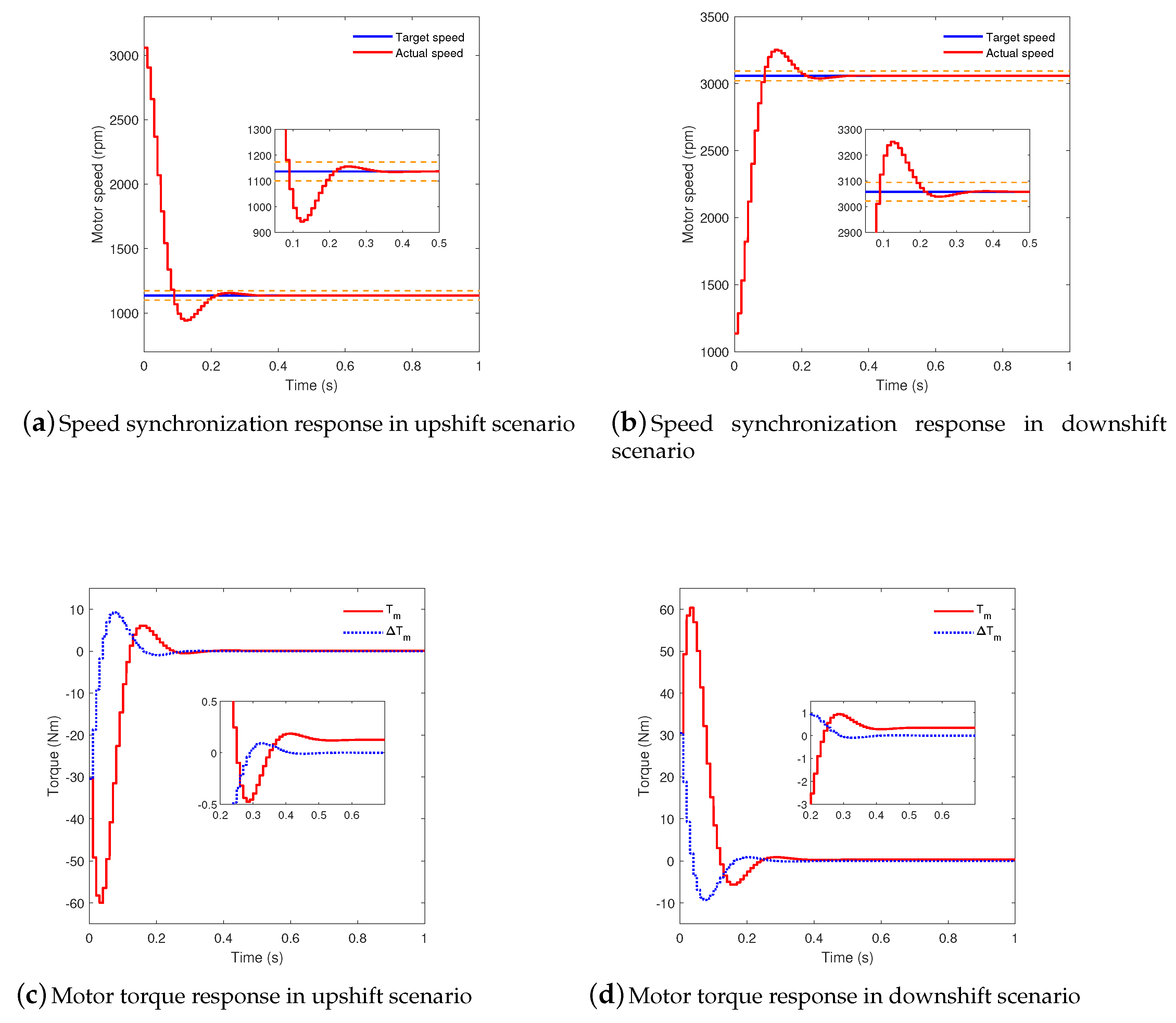
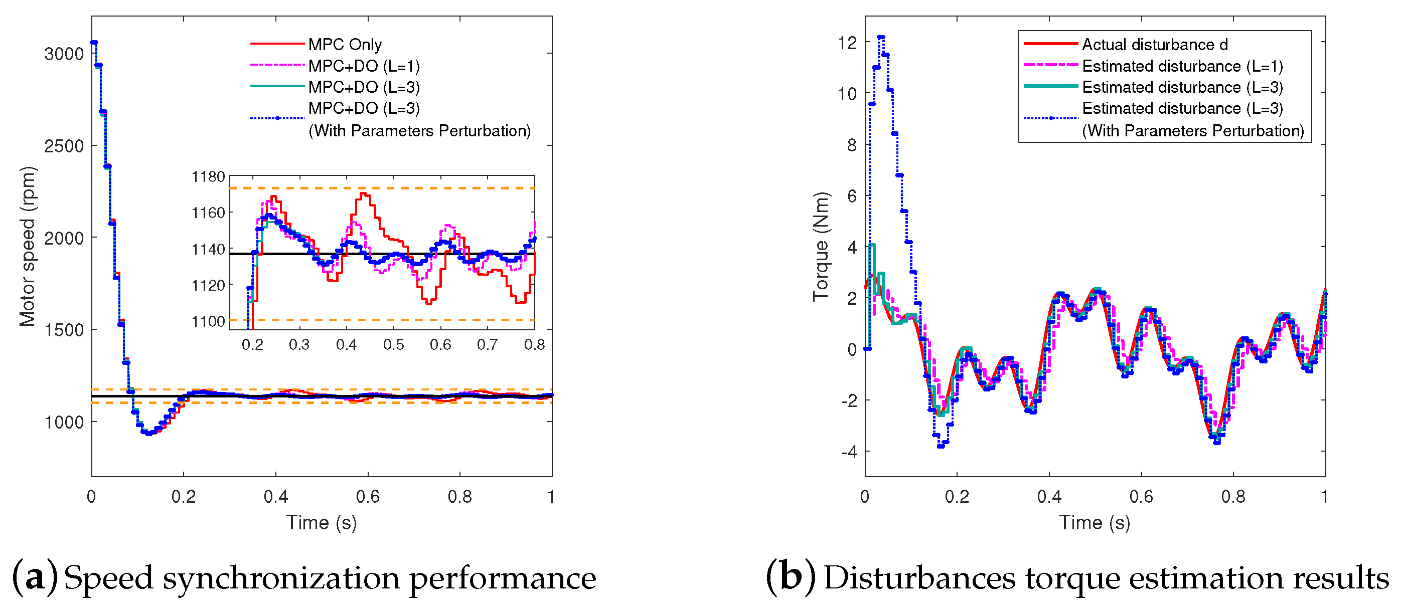
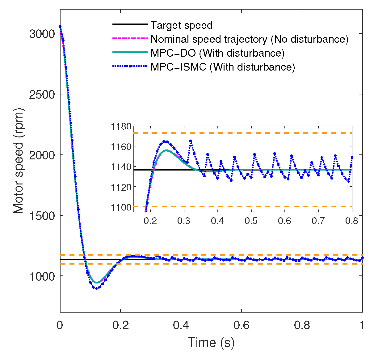
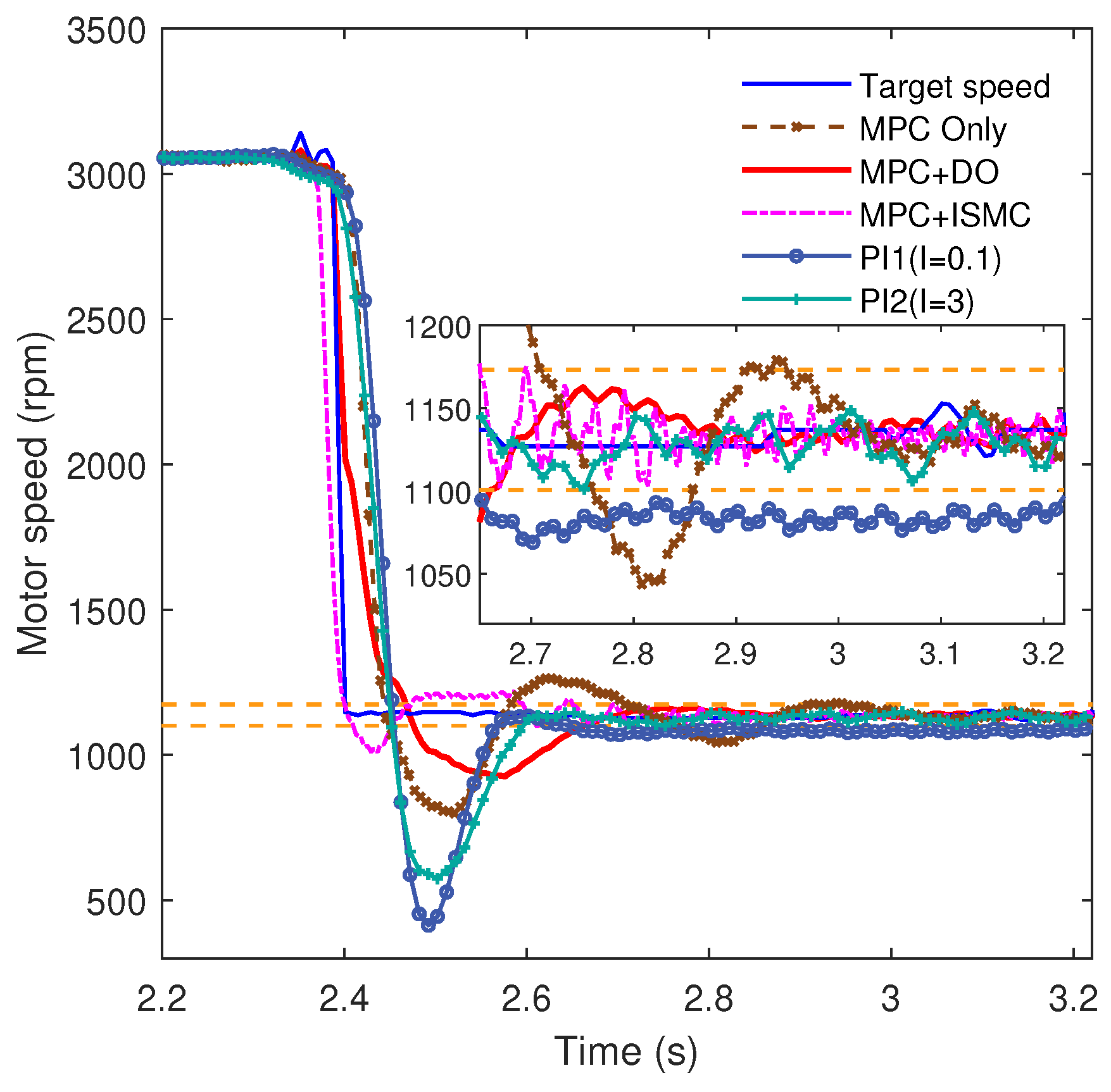
4.1. Simulation Results

The designed speed regulation controller is first tested in a hybrid DCT powertrain model built in MATLAB/Simulink (Version: R2018a). To obtain a small initial speed slip at the beginning of gear engagement phase, the acceptable speed difference in $1\to 3$ upshift and $3\to 1$ downshift is less than 35 rpm according to synchronizer bench test results. In the simulations, the maximum overshoot $\delta$ is chosen to be 10% and the settling time $t_s$ corresponding to the above speed difference bandwidth is 0.2 s. The corresponding closed-loop pole locations are $p_{det}=0.8081\pm 0.2048i$, then the controller parameters can be obtained according to the tuning procedure mentioned above.

Table 2. Main parameters used to generate the desired closed-loop poles (at ${\alpha }_{1,2}<1e-5$).

${\mathit{N}}_{\mathit{p}}$	${\mathit{N}}_{\mathit{c}}$	Q	R	${\mathit{K}}_{\mathit{x}}$	${\mathit{K}}_{\mathit{y}}$
6	2	diag(0.3538,0.2738,0.2336,0.1837,0.1681,0.1434)	diag(8.656,18.42)	[0.5854,0.1514]	0.1514

lists the main parameters for the MPC controller design.

Figure 6 shows that the maximum overshoot and settling time of the system are coinciding with the preset values. Moreover, the motor output torque is relatively small during the speed regulation phase. That is a proof of why an unconstrained MPC is applied rather than a constrained MPC, that is, the motor output torque control sequences are always under the physical limits.

The controller performance is subjected to model parameters’ uncertainty, unmodeled dynamics and measurement noises, and so forth, where these disturbances are usually difficult to measure and analysis in practice. In order to verify the robustness of the controller in presence of disturbances, a hypothetical disturbance is introduced and is assumed as follows:

$$d\left(t\right)=sin(20\pi t+1)+1.5cos\left(4\pi t\right)+sin\left(10\pi t\right).$$

(29)

Equation (29) denotes that the disturbance torque are assumed to be periodic and bounded, where the disturbances are bounded by $\eta =3.438$ Nm. Compared with the amplitude of the motor output torque in the speed regulation phase, the magnitude of the disturbance is consistent with the actual. The results with disturbance compensation are shown in Figure 7 and

Table 3. Speed fluctuation range of different disturbance observer gains.

Controller	Speed Fluctuation Range (rpm)
MPC only	[1109,1170]
MPC + DO (L = 1)	[1123,1158]
MPC + DO (L = 3)	[1131,1143]
MPC + DO (L = 3) with parameters perturbation	[1129,1145]

. It can be observed that the disturbance observer can suppress speed fluctuation. To illustrate the effects of different observer gains, we set the observer gains L to be 1 and 3. The parameters perturbation of $J_{e,m}$ and $b_{e,m}$ are also considered and the disturbance torque estimation results show that the appropriate observer gain can get an excellent estimation effects even there exists a drift in the parameters of the controlled plant model. However, since the characteristics of disturbances are unknown, the observer gain L employed here may be no longer suitable for other disturbance circumstances.

The damping coefficient $b_{e,m}$ has been roughly identified from experimental data, where the damping term is linearly related to speed. As for the disturbance non-linearly relative to speed, because of the lack of the prior knowledge of the nonlinear term of the disturbance, another type of hypothetical disturbance is introduced as:

$$d=f\left({\omega }_m\right),$$

(30)

where the non-linear function is arbitrarily set to be $f=0.0001{(*)}^2$. In the $1\to 3$ upshift and $3\to 1$ downshift process, the disturbance is bounded nearly by $\eta \approx 10$ Nm. To highlight the effectiveness of the proposed disturbance observer, a common disturbance rejection controller integral sliding mode control (ISMC) is introduced, which provide functionality of compensating the matched uncertainties [23].

Figure 8 demonstrates that the proposed disturbance observer can deal with the disturbance torque which is non-linearly relative to speed. While for ISMC method, because of the high-frequency switch control, the motor speed fails to follow the target speed and severe oscillations in speed trajectory occurs.

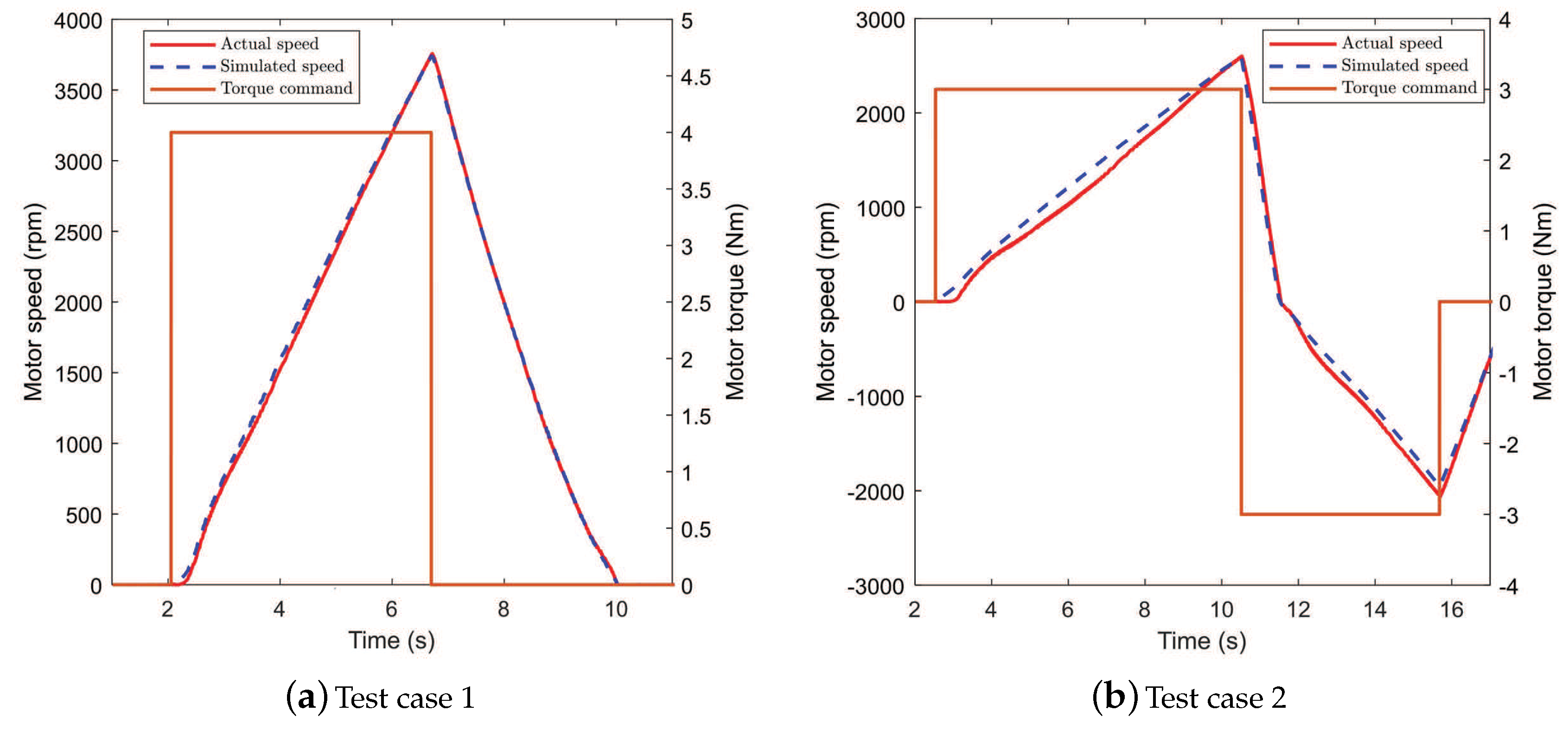
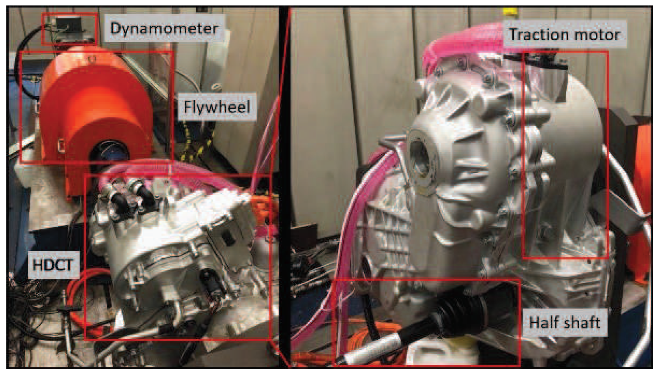
4.2. Experimental Results

To verify the feasibility of the proposed gear shift method in a real application, an experimental platform is built up as Figure 9, including the hybrid DCT gearbox, dynamometer, flywheel and the controlling system. The dynamometer is connected over the output shaft of the hybrid DCT to apply the load and the flywheel is to emulate the vehicle inertia. The proposed algorithm is compiled and deployed into the a real-time MicroAutoBox simulator. Moreover, the delivery of signals between TCU, MCU and the MicroAutoBox simulator is achieved through the CAN bus.

Figure 10 shows the experiment results of a typical $1\to 3$ upshift process. Since the actual disturbance cannot be compensated completely, there are some discrepancies between the simulations and bench test. However, the maximum overshoot and settling time in experiment are roughly coincided with the preset values. The total gear shift time is about 0.8 s, which meets the design specifications and requirements. It can be seen that the speed regulation phase accounts for nearly 63% of the total gear shift time.

To highlight the effectiveness of the proposed combined speed controller, the ISMC method mentioned previously and the PI cascade speed controller [24] are adopted to make a comparison. From Figure 11 and

Table 4. Speed fluctuation range of different methods.

Controller	Speed Fluctuation Range (rpm)
MPC only	[1118,1152]
MPC + DO	[1127,1142]
MPC + ISMC	[1120,1152]
PI1	fail to get the target speed
PI2	[1106,1149]

, it can be seen that the speed synchronization performance employed the combined controller is better than that by employing the only nominal MPC control. The maximum overshoot and the time to stabilize the motor speed to the target value are significantly reduced, which endorses that the disturbance observer can eliminate the disturbance to some extent and improve the gear shift quality. According to the partial enlarged view of Figure 11, it can be guessed that the actual disturbance torque is slowly time-varying since the speed fluctuation of nominal MPC control is within the acceptable speed differences after 3.0 s.

The maximum overshoot of the motor speed responses with PI methods have both surged and only the second PI controller can realize the $1\to 3$ upshift process. The first PI controller failed to adjust the motor speed to the target speed since the static error cannot be eliminated. Sharp speed fluctuation and long transient process cannot be accepted in practice, which can result in a long gear engagement phase. Worse still, a large output torque hole of the vehicle can be emerged since the power flow of the motor is disconnected. As in dictated in Figure 11, the speed fluctuation of the second PI controller is much bigger than that of the combined controller and the time to complete the gear shift event is also far behind that of the MPC method. As for the ISMC method, the maximum overshoot is smaller than the proposed combined speed controller, however, the speed fluctuation range is larger and a slight chattering in speed trajectory occurs.

5. Conclusions

In this work, the speed regulation phase control for a hybrid DCT powertrain in pure electric drive mode is dealt with with a robust speed controller which combines an MPC controller and disturbance observer. Unconstrained MPC is equivalent to unconstrained LQR control with infinite horizon, so it inherits the tuning challenge of the weighting matrices Q and R. The MPC gains obtained with the proposed tuning procedure give a good benchmark for parameters selection in practice. The unknown constant disturbance can be removed by using incremental model, moreover, a discrete-time disturbance observer is used to enhance the robustness of the algorithm. Simulation and experiment results show that the combined control method can realize a fast and robust motor speed regulation process. In addition, the method used in this paper is also applicable to CLAMT systems in other electric vehicles.

References

1. Walker, P.; Zhu, B.; Zhang, N. Powertrain dynamics and control of a two-speed dual clutch transmission for electric vehicles. Mech. Syst. Signal Process 2017, 85, 1–15. [Google Scholar] [CrossRef] [Green Version]
2. Lei, Z.; Sun, D.; Liu, Y.; Qin, D.; Zhang, Y.; Yang, Y.; Chen, L. Analysis and coordinated control of mode transition and shifting for a full hybrid electric vehicle based on dual clutch transmissions. Mech. Mach. Theory 2017, 114, 125–140. [Google Scholar] [CrossRef]
3. Ranogajec, V.; Deur, J. Bond graph analysis and optimal control of the hybrid dual clutch transmission shift process. Proc. Inst. Mech. Eng. Part K J. Multi-Body. Dyn. 2017, 231, 480–492. [Google Scholar] [CrossRef]
4. Piracha, M .; Grauers, A.; Hellsing, J. Improving gear shift quality in a PHEV DCT within tegrated PMSM. In Proceedings of the 16th International CTI Symposium, Automotive Transmissions, HEV and EV drives, Berlin, Germany, 5–12 December 2017; pp. 1–13. [Google Scholar]
5. Liu, H.; Lei, Y.; Li, Z.; Zhang, J.; Li, Y. Gear-Shift Strategy for a clutchless automated manual transmission in battery electric vehicles. SAE Int. J. Commer. Veh. 2012, 5, 57–62. [Google Scholar] [CrossRef]
6. Tseng, C.Y.; Yu, C.H. Advanced shifting control of synchronizer mechanisms for clutchless automatic manual transmission in an electric vehicle. Mech. Mach. Theory 2015, 84, 37–56. [Google Scholar] [CrossRef]
7. Walker, P.; Fang, Y.; Zhang, N. Dynamics and Control of Clutchless Automated Manual Transmissions for Electric Vehicles. ASME. J. Vib. Acoust. 2017, 139, 1–13. [Google Scholar] [CrossRef]
8. Yu, C.H.; Tseng, C.Y. Research on gear-change control technology for the clutchless automatic–manual transmission of an electric vehicle. Proc. Inst. Mech. Eng. Part D J. Autom. Eng. 2013, 10, 1446–1458. [Google Scholar] [CrossRef]
9. Zhu, X.; Zhang, H.; Xi, J.; Wang, J.; Fang, Z. Robust speed synchronization control for clutchless AMT systems in electric vehicles. Proc. Inst. Mech. Eng. Part D J. Autom. Eng. 2014, 229, 424–463. [Google Scholar] [CrossRef]
10. Zhong, Z.; Kong, G.; Yu, Z.; Xin, X.; Chen, X. Shifting control of an automated mechanical transmission without using the clutch. Int. J. Automot. Technol. 2012, 13, 487–496. [Google Scholar] [CrossRef]
11. Zhu, X.; Zhang, H.; Fang, Z. Speed synchronization control for integrated automotive motor–transmission powertrain system with random delays. Mech. Syst. Signal Process 2015, 64, 46–57. [Google Scholar] [CrossRef]
12. Cao, W.; Liu, H.; Lin, C.; Chang, Y.; Liu, Z.; Szumanowski, A. Speed synchronization control of integrated motor–transmission powertrain over CAN through active period-scheduling approach. Energies 2017, 10, 1831–1948. [Google Scholar] [CrossRef] [Green Version]
13. Huang, J.; Zhang, J.; Yin, C. Robust speed synchronization control for an integrated Motor-Transmission powertrain system with feedback delay. In Proceedings of the SAE World Congress Experience (WCX), Detroit, MI, USA, 9–11 April 2019; pp. 1–12. [Google Scholar]
14. Gahagan, M.P. Lubricant technology for hybrid electric automatic transmissions. In Proceedings of the SAE Powertrains, Fuels and Lubricants Meeting, Beijing, China, 16 October 2017; pp. 1–8. [Google Scholar]
15. Alizadeh, H.V.; Boulet, B. Robust Control of Synchromesh Friction in an Electric Vehicle’s Clutchless Automated Manual Transmission. In Proceedings of the IEEE Conference on Control Applications (CCA), Juan Les Antibes, France, 8–10 October 2014; pp. 611–616. [Google Scholar]
16. Zhu, X.; Zhang, H.; Xi, J.; Wang, J.; Fang, Z. Optimal Speed Synchronization Control for Clutchless AMT Systems in Electric Vehicles With Preview Actions. In Proceedings of the American Control Conference, Portland, OR, USA, 4–6 June 2014; pp. 4611–4616. [Google Scholar]
17. Cao, W.; Wu, Y.; Chang, Y.; Liu, Z.; Lin, C.; Song, Q.; Szumanowski, A. Speed Synchronization Control for Integrated Automotive Motor-Transmission Powertrains Over CAN Through a Co-Design Methodology. IEEE Access 2018, 6, 14106–14117. [Google Scholar] [CrossRef]
18. Yu, C.H.; Tseng, C.Y.; Wang, C.P. Smooth Gear-Change Control for EV Clutchless Automatic Manual Transmission. In Proceedings of the IEEE/ASME International Conference on Advanced Intelligent Mechatronics (AIM), Kachsiung, Taiwan, 11–14 July 2012; pp. 971–976. [Google Scholar]
19. Rawlings, J.B.; Mayne, D.Q. Model Predictive Control: Theory and Design, 2nd ed.; Nob Hill Publishing: Madison, WI, USA, 2009. [Google Scholar]
20. Chai, S.; Wang, L.; Rogers, E. Model predictive control of a permanent magnet synchronous motor with experimental validation. Control Eng. Pract. 2013, 21, 1584–1593. [Google Scholar] [CrossRef]
21. Kautsky, J.; Nichols, N.K.; Van Dooren, P. Robust pole assignment in linear state feedback. Int. J. Control 2007, 41, 1129–1155. [Google Scholar] [CrossRef]
22. Wright, S.; Nocedal, J. Numerical Optimization, 2nd ed.; Springer Science: New York, NY, USA, 2006. [Google Scholar]
23. Fridman, L.; Poznyak, A.; Bejarano, F. Robust Output LQ Optimal Control via Integral Sliding Modes; Springer Science: New York, NY, USA, 2014. [Google Scholar]
24. Meshram, M.P.; Kanojiya, G.R. Tuning of PID controller using Ziegler-Nichols method for speed control of DC motor. IEEE Int. Conf. Control Appl. 2012, 1, 117–122. [Google Scholar]
Figure 1. Schematic of the hybrid DCT powertrain system. (a) The power flow of the hybrid DCT in pure electric drive mode; (b) The 3-D model of the hybrid DCT gearbox.
Wevj 11 00011 g001
Figure 2. The hybrid DCT powertrain system over a controller area network (CAN).
Wevj 11 00011 g002
Figure 3. The gear shift process flowchart of the hybrid DCT in pure electric drive mode.
Wevj 11 00011 g003
Figure 4. Simulated model response versus measured data. (a) Test case 1; (b) Test case 2.
Wevj 11 00011 g004
Figure 5. Block diagram of the combined speed regulation controller.
Wevj 11 00011 g005
Figure 6. The 1–3 upshift and downshift process with the desired poles. (a) Speed synchronization response in upshift scenario; (b) Speed synchronization response in downshift scenario; (c) Motor torque response in upshift scenario; (d) Motor torque response in downshift scenario.
Wevj 11 00011 g006
Figure 7. Speed synchronization performance with the proposed disturbance observer. (a) Speed synchronization performance; (b) Disturbances torque estimation results.
Wevj 11 00011 g007
Figure 8. Speed synchronization performance with MPC + DO and MPC + ISMC methods.
Wevj 11 00011 g008
Figure 9. Test bench for the hybrid DCT powertrain system.
Wevj 11 00011 g009
Figure 10. The 1–3 upshift process in experiment. (I: Gear releasing phase, II: Speed regulation phase, III: Gear engagement phase).
Wevj 11 00011 g010
Figure 11. Experiment results for different methods.
Wevj 11 00011 g011