YOLOv8-Based Defect Detection for the Selection of Defect-Free Beech Wood Specimens: Experimental and Numerical Validation

Abstract

Wood is a renewable and widely used material whose mechanical performance is strongly influenced by natural defects such as knots, cracks, and resin pockets. These defects affect structural accuracy and make quality assessment an essential step in wood processing and engineering applications. Traditional visual inspection methods are time consuming and subject to individual variability, motivating the development of automated inspection systems based on computer vision. This study proposes a YOLOv8-based framework for automated wood classification and specimen selection. Two YOLOv8 variants, Nano and Medium, were trained on a publicly available wood defect dataset containing more than 20,000 images and over 43,000 annotated defects. The models were used to distinguish defect-free specimens from specimens containing visible defects, enabling objective sample selection. Only specimens classified as defect-free were retained for subsequent three-point bending tests and finite element method (FEM) simulations. Both YOLOv8 models achieved reliable detection performance, allowing consistent separation of defective and defect-free wood samples. The selected specimens exhibited stable mechanical behavior during bending tests, while FEM predictions showed good agreement with the experimental results, with errors below 3.2% in the elastic range. The proposed methodology demonstrates the potential of integrating artificial intelligence, mechanical testing, and numerical simulation into a unified workflow for wood quality assessment and structural evaluation.

1. Introduction

Wood is one of the most essential resources used in our daily life. It serves as the main resource used in various industries such as energy, construction, tools, transportation and furniture. Such longevity is due to its natural renewable property. There are many tree species, each exhibiting unique physical and mechanical properties, including density, stiffness, strength, durability, and moisture behavior. In addition, wood is susceptible to defects such as knots or rot, which affect their level of usability [1,2].

Knots are natural imperfections in wood that form where branches were once attached to the tree trunk. Knots weaken and disrupt the normal grain structure, create localized changes in density, and vary in size, shape, and integrity. Because knot characteristics are closely related to timber stiffness, strength, and bending failure mechanisms, computer vision techniques have the potential to support mechanical characterization and grading of wood products [3,4]. Wood defects, particularly knots, significantly influence the mechanical performance and structural reliability of timber. Consequently, non-destructive evaluation methods have become increasingly important for timber grading and strength assessment, providing a foundation for modern machine vision and automated defect detection approaches [5,6,7].

Machine learning has emerged as a valuable tool for non-destructive wood evaluation, enabling improved defect detection, property prediction, and timber grading while supporting the digitalization of wood science and engineering [8,9]. Deep learning has become a fundamental technology in computer vision, providing highly effective methods for image classification, object detection, and pattern recognition. Combined with advances in computer vision algorithms, these techniques have enabled the development of real-time detection frameworks, which are increasingly adopted in quality control inspection [10,11].

Recent advances in computer vision have enabled automated solutions for wood quality assessment. Deep learning-based object detection algorithms, such as YOLO (You Only Look Once), provide high detection accuracy and real-time performance [12,13,14]. Their application to wood defect detection has demonstrated significant potential for improving industrial inspection processes and timber quality classification.

Over the past years, researchers have carried a substantial number of studies devoted specifically to wood defect detection with optimized YOLO variants. These approaches aim to enhance feature extraction and localization capabilities while maintaining the real-time inference characteristics of the original architecture. Wang et al. [15] proposed ODCA-YOLO, built on YOLOv7, adding an omni-dynamic convolution coordinate attention mechanism together with an efficient feature-extraction block. They reported a mAP of 78.5%, roughly 9 percentage points above the baseline, with the emphasis placed on small defects and on richer feature representation [15]. In addition, in the focused research of Meng and Yuan, they proposed SGN-YOLO, which integrates a Semi-Global Network into the YOLOv5 architecture to strengthen contextual feature learning and improve defect detection accuracy in complex wood surface images [16].

The study of An et al. [17] proposed CWB-YOLOv8, an improved YOLOv8-based algorithm specifically developed for wood defect detection. By enhancing feature representation and detection capability, the proposed model improved the identification of wood surface defects and demonstrated superior performance compared with the original YOLOv8 architecture, confirming the effectiveness of specialized deep-learning solutions for automated wood inspection.

While these enhanced YOLO architectures demonstrate improved defect-detection performance, they generally achieve these gains through the introduction of additional attention mechanisms, feature-fusion modules, customized convolution layers, or modified loss functions. Such modifications inevitably increase model complexity, computational cost, and implementation requirements, which may limit their applicability in practical industrial environments. Furthermore, many of these architectures have been validated primarily on specific datasets, making direct comparisons and broader deployment more challenging.

In contrast, the native YOLOv8n and YOLOv8m models provide a well-established balance between detection accuracy, computational efficiency, reproducibility, and ease of deployment. Since the objective of the present work was not to propose a new defect-detection architecture but rather to evaluate the feasibility of integrating automated defect recognition with mechanical testing and finite element analysis, the standard YOLOv8 implementations were selected as representative and widely accessible object-detection frameworks.

Wang et al. [18] proposed an improved YOLOv8-based approach for wood surface defect detection, integrating multi-scale feature extraction and fusion modules, dynamic detection heads, and an MPDIoU loss function. The enhanced model achieved a 5.5 percentage point improvement in mAP compared with the baseline YOLOv8n architecture. Xi et al. [19] developed SiM-YOLO, an improved YOLOv8-based method that incorporates SPD-Conv, attentional feature fusion, and a multi-attention detection head. The proposed architecture achieved a 4.3 percentage point increase in mAP compared with the original YOLOv8 model, demonstrating the continued effectiveness of specialized YOLO variants for wood defect inspection.

Three-point bending testing is widely employed for the characterization of wood mechanical properties, providing important parameters such as the modulus of elasticity, modulus of rupture, and bending toughness. Recent studies have applied this methodology to European beech (Fagus sylvatica), demonstrating its effectiveness for evaluating flexural performance and validating non-destructive assessment techniques [20].

To accurately assess the fundamental mechanical behavior of wood, several researchers have focused on clear specimens free from visible defects. Knapic et al. [21] evaluated the compressive and bending strength of Portuguese clear oak wood, demonstrating the relevance of defect-free samples for characterizing inherent material properties and reducing the influence of structural imperfections on test results.

Furthermore, the integration of finite element modelling with experimental bending tests has become increasingly common, enabling detailed analyses of stress distributions, deformation behavior, and failure mechanisms. Kubík et al. validated an orthotropic finite element model against three-point bending tests performed on European beech, highlighting the effectiveness of numerical simulations for predicting deformation and fracture behavior [22]. Töpler et al. highlighted the importance of material characterization, verification, and validation in the development of reliable finite element models for beech-based timber products [23].

Hu and Liu [24] evaluated different finite element modelling strategies for predicting the bending strength of mortise-and-tenon joints and reported good agreement between numerical predictions and experimental observations, confirming the suitability of FEM for wood-related structural analyses.

Combining experimental bending tests and numerical modelling has proven effective for investigating the mechanical behavior of wood products. Réh et al. [25] analyzed beech laminated elements through three-point bending experiments coupled with numerical simulations, demonstrating the relevance of this integrated methodology for evaluating flexural strength and deformation characteristics. Hu et al. validated finite element models against experimental measurements of beech wood, demonstrating that FEM can accurately predict the material response under different loading scenarios and can serve as a valuable complement to mechanical testing [26].

Despite the considerable progress achieved in wood defect detection using advanced YOLO-based architectures, most of the previous studies have primarily focused on improving detection accuracy and classification performance. Similarly, experimental bending investigations and finite element analyses have generally been conducted independently of automated specimen selection procedures. As a result, the direct influence of AI-based defect screening on the reliability of mechanical testing and numerical model validation remains largely unexplored. Furthermore, few studies have established a complete workflow linking automated defect detection, experimental characterization, and finite element verification within a single framework. Therefore, there is a need for an integrated methodology capable of objectively identifying defect-free specimens, reducing the variability introduced by natural wood defects, and improving the consistency between experimental and numerical analyses. To address this gap, the present study proposes a unified framework combining YOLOv8-based defect detection, three-point bending testing, Digital Image Correlation measurements, and finite element modelling for the structural assessment of beech wood specimens. In addition, this can establish a baseline framework that can be extended in future work to incorporate image-derived defect geometry and experimentally determined material properties.

2. Materials and Methods

2.1. Automated Wood Classification Using YOLOv8

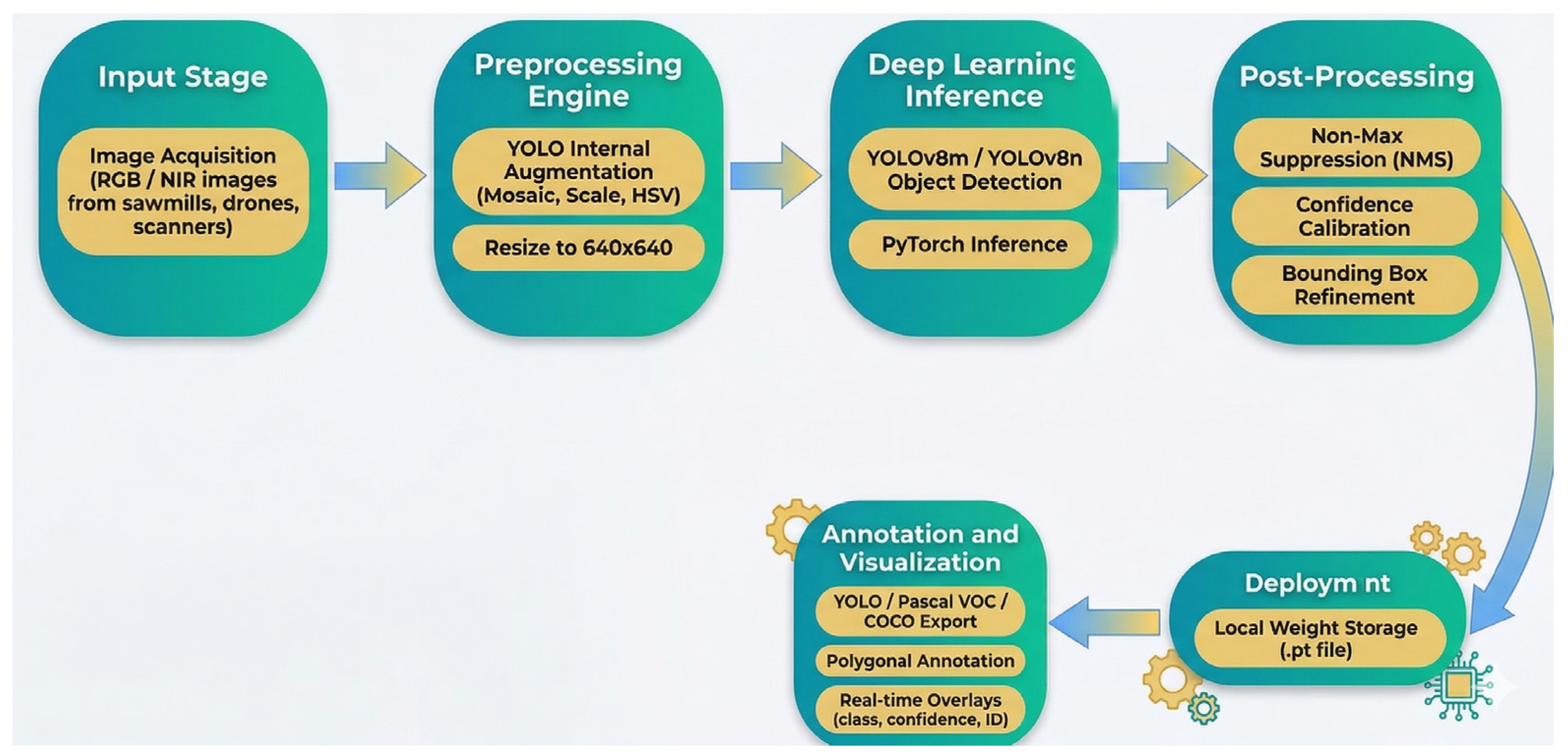
To support the selection of specimens for mechanical testing, an automated wood classification framework was developed using a Python Flask service (version 3.12.10; Python Software Foundation) integrating image preprocessing, object detection, annotation, and visualization into a single workflow. The system was designed to distinguish between defect-free specimens and specimens containing visible defects, thereby enabling objective specimen selection prior to experimental testing and numerical modelling. Recent advances in deep learning-based object detection, particularly the YOLO family of algorithms, have demonstrated high accuracy and computational efficiency in wood defect inspection applications, making them suitable for industrial quality-control systems [13,16].

Figure 1 presents the proposed workflow, which begins with image acquisition and concludes with defect annotation and visualization. Following acquisition, all images were resized to 640 × 640 px to satisfy the input requirements of the YOLOv8 architecture. Two model variants, YOLOv8n (Nano) and YOLOv8m (Medium), were evaluated using the PyTorch framework (version 2.13.0; PyTorch Foundation). The post-processing stage included confidence calibration and bounding-box refinement to improve detection reliability [27].

Since wood surface images are frequently acquired under non-controlled environmental conditions, preprocessing techniques including noise reduction and color calibration were applied to minimize variations caused by illumination and image quality. The dataset was obtained from a publicly available repository [27] and contains more than 20,000 images with over 43,000 annotated defects. The available annotations include live knots, dead knots, knots with cracks, resin pockets, cracks, missing knots, brittle heart, overgrown knots, and blue stain defects. Similar datasets have been widely employed in recent studies for the development and evaluation of YOLO-based wood inspection systems [16,17,19].

For the purposes of the present study, the defect categories were grouped into a binary classification scheme consisting of defect-free wood and defective wood, where defective specimens contained at least one of the annotated defect types. The objective was not only to detect defects but also to identify specimens suitable for subsequent mechanical characterization. Consequently, only samples classified as defect-free were retained for the three-point bending experiments and finite element simulations, while all defective specimens were excluded from further analyses. This approach is consistent with previous studies highlighting the importance of clear wood specimens for obtaining reliable and representative mechanical properties during bending tests [21].

The dataset was divided into training and validation subsets using a 90:10 ratio. The split was performed at specimen level rather than image level, meaning that all images acquired from the same board, including different views and illumination conditions of the same defect, were assigned to the same subset. This approach prevented near-duplicate images of the same physical defect from appearing in both training and validation sets, thereby avoiding data leakage and artificially inflated performance metrics. Within this constraint, specimens were randomly assigned using a fixed random seed (seed = 0) to ensure reproducibility. The resulting class distributions were verified after partitioning and remained representative of the complete dataset. Data augmentation was applied only to the training subset and only after dataset partitioning; consequently, no augmented versions of validation images were exposed to the model during training.

Both YOLOv8 models were trained under identical conditions using the Ultralytics implementation with a PyTorch backend and COCO-pretrained weights. Training was performed for 100 epochs at an input resolution of 640 × 640 px using a batch size of 16 and stochastic gradient descent (SGD) optimization with an initial learning rate of 0.01, momentum of 0.9, and weight decay of 5 × 10⁻⁴. Mixed-precision training and standard YOLOv8 data augmentation techniques, including mosaic augmentation, random scaling, translation, horizontal flipping, and HSV adjustments, were employed. A fixed random seed was used to ensure reproducibility.

The trained YOLOv8 models were subsequently used to screen the prepared specimens and identify those free from visible defects. Only specimens classified as defect-free were retained for mechanical characterization and numerical analysis.

2.2. Raw Material

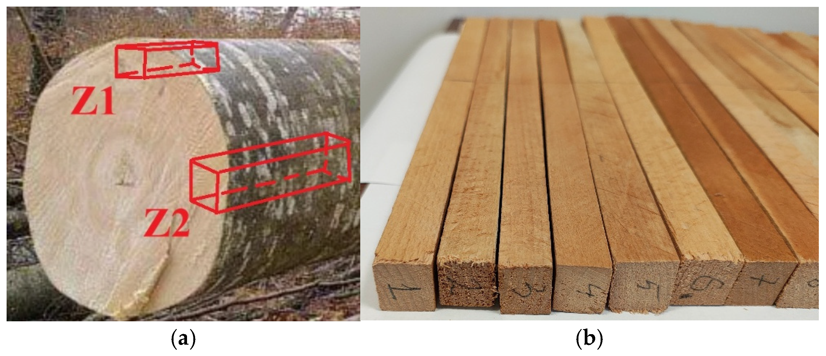
The raw material used in this study was beech wood (Fagus sylvatica L.) obtained from a legally harvested tree in accordance with Romanian forestry regulations. Beech wood was selected due to its relatively homogeneous structure, high mechanical strength, and extensive availability in European forests, which make it a suitable material for investigating the relationship between automated defect detection, experimental characterization, and numerical modelling while limiting the influence of excessive natural defects commonly encountered in softwood species. The investigated tree had an estimated age of over 100 years. The moisture content of the specimens corresponded to the moisture content of the processed wood supplied for industrial applications and did not exceed 15%. All specimens were conditioned under the same environmental conditions prior to testing to ensure consistency of the experimental results. Experimental specimens were prepared from a single beech log. Since wood properties are influenced by the location within the stem, special consideration was given to the sampling position. The specimens were cut from precisely defined areas of the log, taking into account the radial position and the distance from the pith, in order to minimize material variability and ensure the comparability of the test results. The selected sampling zones were representative of the investigated wood material and were maintained consistently throughout the specimen preparation process.

In Zone 1, the specimens were cut so that the growth rings were distributed radially along the specimen height, whereas the fibers were oriented in the longitudinal direction. In Zone 2, the growth rings are distributed radially across the base of the specimen, whereas the fibers are oriented in the longitudinal direction. The location and orientation of the specimens within the log were carefully controlled, since these factors can significantly influence the physical and mechanical behavior of wood. The two zones from the beech log are highlighted in Figure 2.

The anatomical orientation of the specimens was carefully controlled during the cutting process. For all specimens, the wood fibers were aligned with the longitudinal axis, while the radial and tangential directions were maintained according to the sampling configuration illustrated in Figure 2. Consequently, specimens originating from the same extraction zone exhibited similar grain orientation on the analyzed surfaces, ensuring consistent conditions for DIC measurements and finite element modelling.

2.3. Specimen Preparation

Prior to testing, all specimens were conditioned under controlled laboratory conditions at a temperature of 23 °C and a relative humidity of 60%. The moisture content of the specimens corresponded to that of the processed wood supplied for industrial applications and did not exceed 15%. The specimens were prepared and their dimensions were measured. A thin white base layer was then applied to the surface, followed by the application of randomly distributed black speckles, creating a high-contrast stochastic pattern. This pattern served as a reference for the Digital Image Correlation (DIC) technique, allowing accurate determination of displacement and strain fields throughout the loading process.

All specimens had a length exceeding 250 mm. A total of 50 specimens were sampled from the log, but only a total of 26 specimens classified as defect-free by the YOLOv8-based inspection framework were selected for the experimental campaign. The rejected specimens contained at least one visible defect identified by the YOLOv8 framework, including knots, cracks, resin pockets, blue stain, or related defect categories present in the training dataset. The dimensions of the cross-sections are listed in

Table 1. Specimen dimensions used for three-point bending test.

Specimen	Zone	b—Base (mm)	h—Height (mm)
1	2	21.11	24.13
2	2	20.45	23.45
3	2	20.68	24.25
4	2	22.19	24.23
5	2	23.00	24.57
6	2	19.83	24.17
7	2	19.41	24.32
8	2	21.45	23.98
9	2	21.41	24.42
10	2	21.13	24.98
11	2	23.69	24.02
12	2	21.03	24.17
13	2	21.47	24.52
14	1	24.97	21.40
15	1	24.63	20.08
16	1	24.41	20.88
17	1	24.03	20.75
18	1	23.82	20.98
19	1	25.11	19.73
20	1	24.21	21.48
21	1	25.19	23.42
22	1	23.33	20.43
23	1	24.19	23.04
24	1	24.23	21.46
25	1	25.00	18.86
26	1	24.95	18.73

.

The dimensional variability observed among the specimens reflects the geometry obtained directly from the sawing process and was intentionally preserved to better represent practical timber products used in construction applications. Prior to testing, all specimens were conditioned under controlled laboratory conditions (23 °C and 60% relative humidity). Therefore, the dimensional differences were associated with the preparation process rather than moisture-related effects. The actual dimensions of each specimen were individually measured and directly incorporated into the stress and strain calculations used to generate the stress–strain curves. Therefore, the dimensional variability did not affect the accuracy of the reported mechanical properties.

2.4. Three-Point Bending Testing

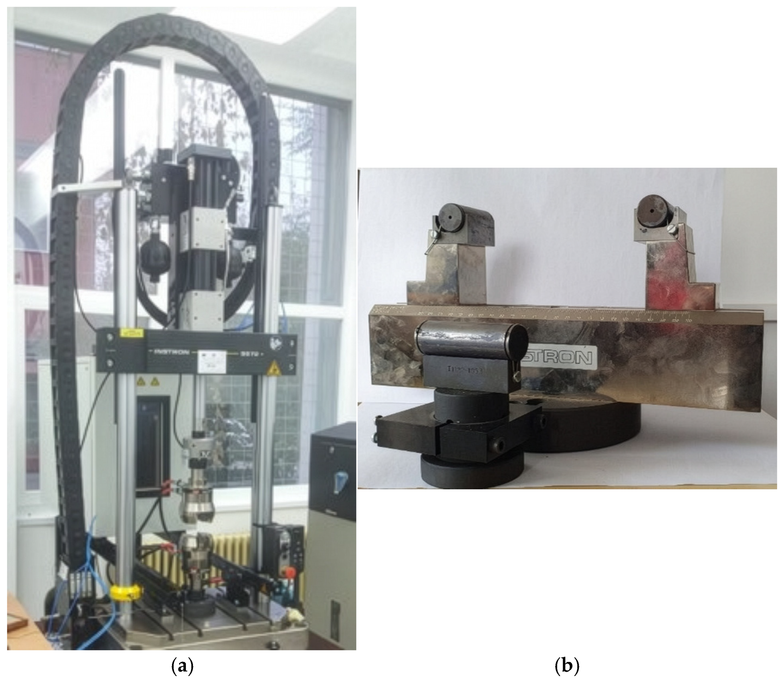
The three-point bending tests were performed in accordance with ISO 13061-3/2014. The tests were conducted using an INSTRON 8872 (Instron, Norwood, MA, USA) electrohydraulic universal testing machine (UTM), shown in Figure 3a, equipped with a ±25 kN load cell. For performing the test, it was used the Three-Point Bending Fixture, accessory of the UTM, presented in Figure 3b.

The distance between the lower supports was 250 mm. The tests were performed under displacement control at a crosshead speed of 4 mm/min. Force measurements were recorded at an acquisition rate of 5 Hz throughout the test duration.

Three-point bending was selected instead of four-point bending because concentrated loading conditions are frequently encountered in practical timber structures and engineering applications. Moreover, the localized load application generates well-defined strain concentrations beneath the loading point, providing a suitable configuration for validating the strain fields obtained using Digital Image Correlation (DIC) and finite element modelling.

Although ISO 13061-3 recommends standardized specimen dimensions, the specimens were intentionally not machined to uniform sizes to preserve the dimensional variations resulting from the sawing process. The actual dimensions of each specimen were measured and used in all stress and strain calculations.

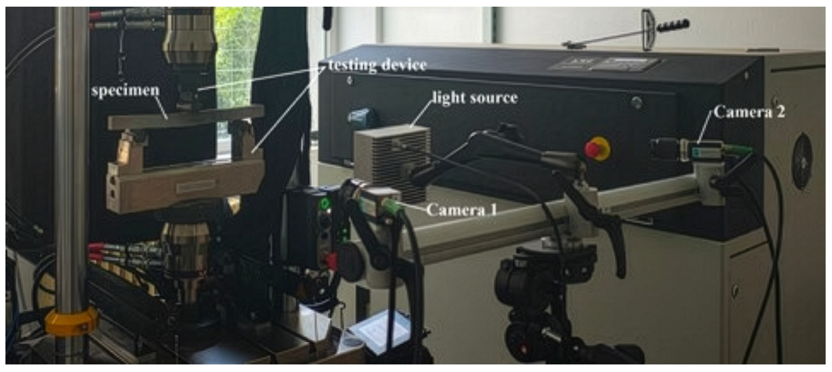
Strain and deformation measurements during the three-point bending tests were performed using the Digital Image Correlation (DIC) technique. This method is based on the acquisition of successive images of the specimen surface during loading. A stereoscopic system, manufactured by Dantec Dynamics (Skovlunde, Denmark), consisting of two cameras was used to capture the specimen deformation and to calculate the full-field three-dimensional displacement and strain distributions (Figure 4).

The acquired images were processed using the ISTRA 4D software platform, which was used to evaluate the full-field displacement and strain distributions throughout the three-point bending tests.

The DIC system consisted of two cameras and a red-spectrum illumination source. The stereoscopic imaging setup enabled the quantification of full-field three-dimensional deformations by measuring displacements along the x and y axes in the specimen plane and along the z axis normal to the specimen surface, directed toward the cameras.

To enable the application of the Digital Image Correlation (DIC) technique, the specimen surfaces were prepared by applying a uniform background coating, typically white, followed by the deposition of randomly distributed black speckles to create a high-contrast stochastic pattern. The method involves selecting a reference image, usually the first acquired frame, and subsequently analyzing consecutive images to determine the deformation behavior of the specimen during loading.

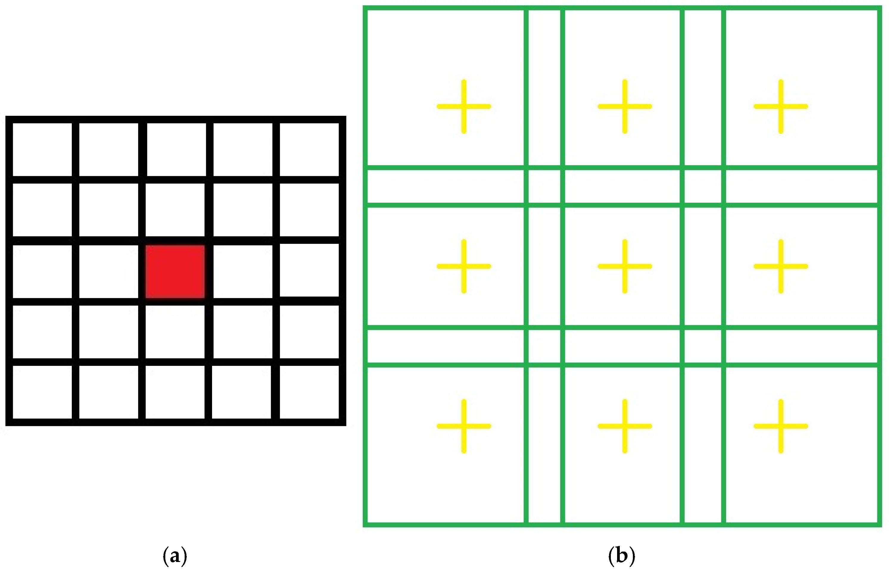
The fundamental principle of DIC consists of dividing the reference image into square subsets (facets) of predefined size and spacing. Starting from a central pixel, neighboring pixels are progressively included until the specified facet size is reached. These facets are then tracked throughout the image sequence to calculate displacement and strain fields. Each facet contains an odd number of pixels, ensuring the existence of a unique central pixel, while the spacing between adjacent facets is defined as the distance between their respective central pixels.

The spacing between adjacent facets was selected such that neighboring facets shared approximately one-third of their pixels, ensuring sufficient overlap for robust correlation analysis. Figure 5 illustrates a facet with dimensions of 5 × 5 pixels, with the central pixel highlighted in red and the corresponding of adjacent facets. Digital Image Correlation (DIC) measurements were performed using a VCXU-50M camera with a resolution of 2448 × 2048 pixels. Images were acquired at a rate of 2 Hz, with the camera positioned approximately 800 mm from the specimen surface. Strain field evaluation was carried out using a facet size of 31 pixels and a grid spacing of 17 pixels.

Using the reference image, the ISTRA 4D software generated facets according to the criteria described above and subsequently searched for the corresponding pixel patterns in each successive image. Based on the initial calibration of the stereo imaging system, the software determined the displacement of each facet relative to its position in the reference image. These displacement data were then used to calculate the full-field deformation and strain distributions developing on the specimen surface throughout the loading process.

In addition to the full-field measurements provided by the DIC system, the global bending response of each specimen was evaluated using the classical strength-of-materials formulation for a simply supported beam subjected to three-point bending. The maximum normal stress was calculated at the midspan section on the tensile side of the specimen according to:

$$\mathsf{\sigma }={\displaystyle \frac{3\mathrm{FL}}{2\mathrm{b}{\mathrm{h}}^2}}$$

(1)

where F is the applied load (N), L is the support span (mm), b is the specimen width (mm), and h is the specimen height (mm).

The outer-fiber strain was determined from the midspan deflection using:

$$\mathsf{\epsilon }={\displaystyle \frac{6\mathrm{hf}}{{\mathrm{L}}^2}}$$

(2)

where h is the specimen height (mm), f is the midspan deflection (mm), and L is the support span (mm).

The stress–strain curves presented in Section 3 were obtained by plotting the calculated bending stress as a function of the corresponding strain values.

2.5. Finite Element Analysis

2.5.1. Geometry, Mesh and Boundary Conditions

A finite element (FE) model was developed by employing ANSYS Mechanical APDL 19.0 to reproduce the experimental three-point bending tests and investigate the mechanical response of the beech wood specimens. Two representative experimental configurations were considered (specimen 2 and 16). The numerical model was formulated as a two-dimensional plane-stress problem, with the longitudinal direction of the specimen (L) aligned with the global (X)-axis and the transverse direction (R) aligned with the global (Y)-axis. A rigid body definition was employed for modelling the machine head and supporting rollers geometries.

Table 2. Geometric data of the studied specimens.

Specimen	Dimensions (mm)
	Length	Width	Thickness
2	360	20.45	23.45
16	360	24.41	20.88

summarizes the simulation model input data.

The assembly was meshed by employing four-node PLANE182 structural elements formulated under plane-stress conditions. A global element size of 1 mm was decided for the entire model. Mesh refinement was carried out in the body interaction regions corresponding to the loading head and the supporting rollers, where peak stress gradients are expected (Figure 6).

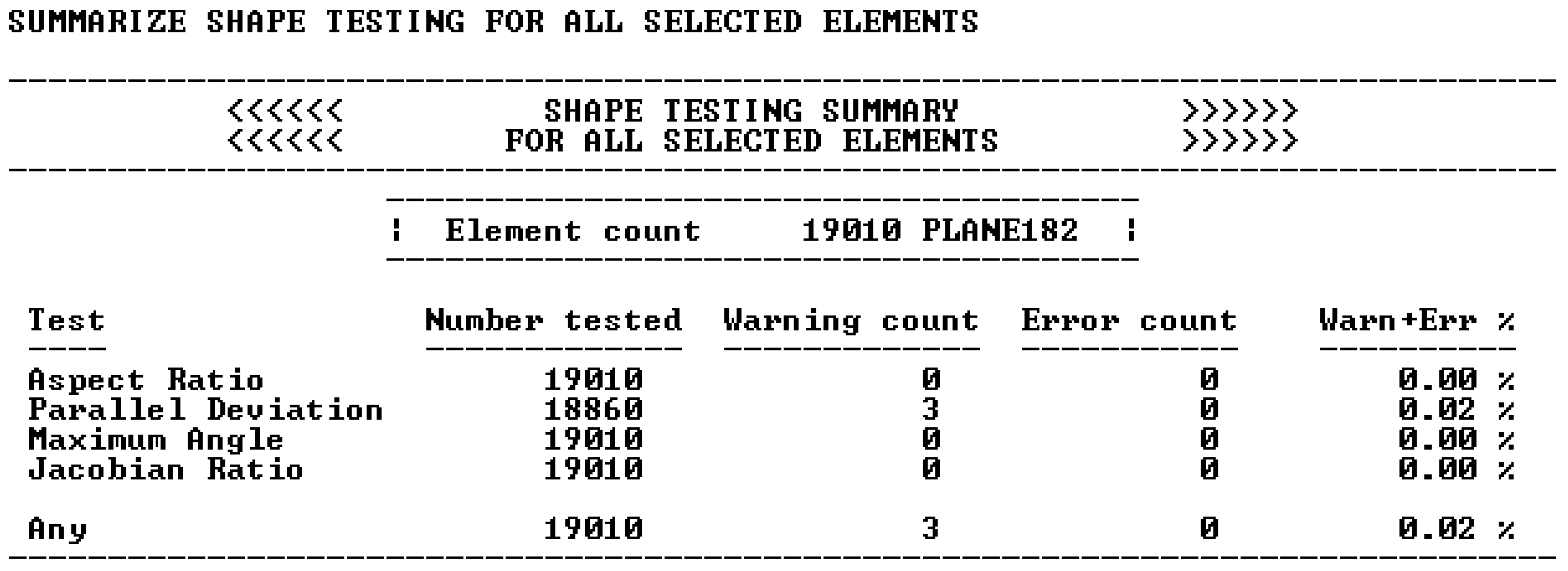
In these locations, the local element size was set to 0.25 mm. Mesh quality metrics were processed by employing the shape testing (SHPP) command. Criteria such as aspect ratio, maximum corner angle, parallel deviation, Jacobian ratio and warping were verified against the default references from ANSYS APDL 19.0 (ANSYS, Inc., Canonsburg, PA, USA). Figure 7 depicts that only three elements or 0.02% have parallel deviation issues, meaning that 99.98% of the elements respect all quality criteria.

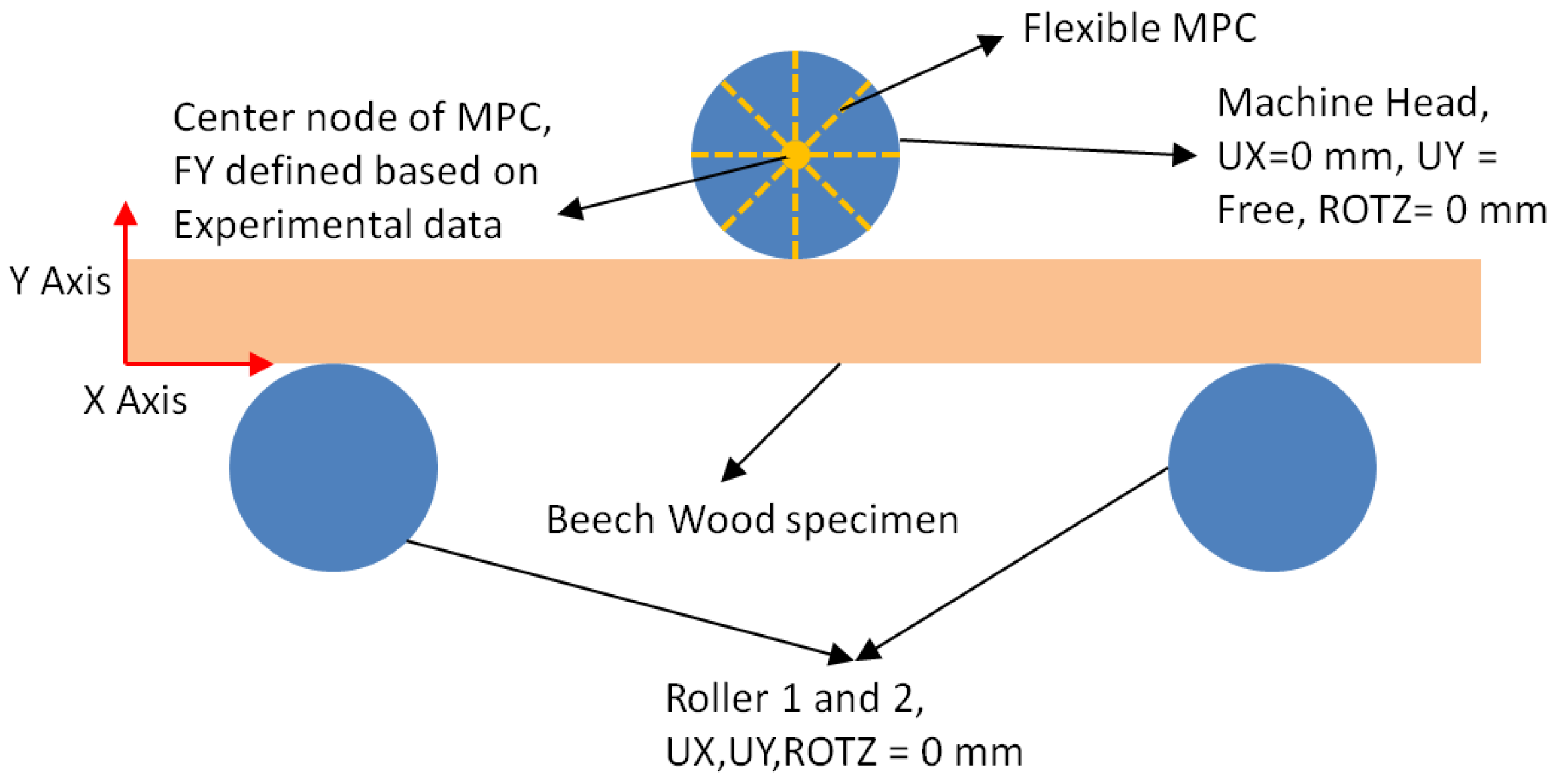
Rigid-body motion was constrained for the supports while the loading head was allowed to displace along the loading direction. The bending load was induced at the centroid of the loading head. A flexible multipoint constraint (MPC) formulation was employed to transfer the prescribed loading to the loading-head geometry. The applied load levels were defined according to the forces recorded during the experimental procedures. A symmetric loading configuration was defined with respect to the midspan of the specimen and the support span employed experimentally.

Figure 8 depicts a representation of the loads and boundary conditions.

Contact interactions between the specimen and the loading/support components were represented by means of CONTA172 and TARGE169 contact–target element pairs. The contact regions were defined over the geometrically imprinted interaction edges.

The Augmented Lagrange formulation was employed for enforcement of the contact constraints, with contact detection performed at the Gauss integration points. A coefficient of friction of 0.45 was adopted for the steel-wood interfaces, based on values reported in the literature for European beech and numerical simulations involving wood contact interactions (Kubík et al. [28]). The contact tracking formulation was defined using the small-sliding assumption, consistent with the limited relative tangential motion expected at the interfaces during the considered loading range.

The simulations were completed by using a nonlinear static analysis, with the large-displacement enabled to account for the frictional body interaction and the incremental application of the applied load.

Automatic time stepping was employed, with an initial increment corresponding to 1 × 10⁻³% of the total applied load, a minimum increment of 1 × 10⁻⁷% and a maximum increment of 1 × 10⁻²%. These settings were decided to facilitate convergence of the nonlinear contact while providing sufficient resolution for the comparison of the experimental and simulation results.

The main numerical quantities that were requested for comparison with the experimental measurements were the bending displacement (Δy) and the principal strain components in the longitudinal (ε₁).

Direct comparison between the force-deflection curves was completed to evaluate the ability of the FE model to reproduce the global structural response. Quantitative agreements were assessed using the percentage error between the experimentally measured and numerically predicted responses at selected load levels.

In addition to the global response, the spatial distributions of ε₁ derived from the FE simulations were compared with the strain distributions evaluated by means of DIC.

2.5.2. Material Model

Beech wood was modeled by using a linear elastic orthotropic material aligned according to the L, R and T anatomical directions of the wood specimens. The initial elastic constants required by the orthotropic constitutive model, including the Modulus of Elasticity, Poisson’s ratios, and Shear Modulus, were established based on the existing experimental data and representative values reported in the literature for beech wood (

Table 3. Material properties employed.

Specimen	Modulus of Elasticity (MPa)			Poisson Ratio			Shear Modulus (MPa)
Direction	L	R	T	LR	LT	RT	LR	LT	RT
Literature reference [24]	12,205	1858	774	0.502	0.705	0.526	899	595	195
2	11,578	1760	737	0.499	0.7	0.523	998	659	216
16	13,406	2036	848	0.401	0.563	0.42	747	494	162

) [24].

A generic structural steel linear elastic material model was assigned for the rollers and the machine head.

The FEM analysis in this work is not aimed at proposing a new finite element formulation, but to show the numerical part of the proposed integrated workflow in a controlled three-point bending configuration. In the simplified 2D representation adopted, the relevant features of the physical test, such as specimen-support and specimen-loading-head interactions, frictional contact and geometrically nonlinear large displacement analysis were maintained. The present setting provides a computationally cheap proof of concept for experimental–numerical comparison and defines a modelling framework which can be extended to more complex geometries, loading conditions and contact interactions.

3. Results

3.1. YOLOv8-Based Defect Detection and Specimen Selection

Both YOLOv8 variants, YOLOv8m and YOLOv8n, demonstrated reliable performance for automated wood defect detection following 100 training epochs, reaching stable convergence without signs of overfitting. YOLOv8m achieved a maximum mAP@50 of approximately 0.74 and a peak F1-score of 0.70, while YOLOv8n obtained a mAP@50 of 0.71 and an F1-score of approximately 0.69. The results indicate that both models were capable of accurately identifying the most frequent defect categories, particularly live knots, dead knots, and knots with cracks. Lower detection performance was observed for underrepresented defect classes, such as brittle heart and missing knots, which can be attributed to the class imbalance present in the training dataset.

Despite their architectural differences, both models effectively distinguished specimens containing defects from defect-free specimens, which represented the primary objective of this study. YOLOv8m provided slightly higher detection accuracy and confidence, making it more suitable for applications where classification reliability is critical. In contrast, YOLOv8n achieved comparable performance with a substantially lower computational cost, making it a promising solution for edge-based or real-time industrial deployment.

The obtained results demonstrate that the YOLOv8 framework can be successfully employed as an automated quality-control tool for wood inspection. By reliably identifying defects such as knots, cracks, resin pockets, missing knots, and blue strain, the models enabled the systematic separation of specimens into defective and defect-free categories. This automated classification process reduced the subjectivity associated with visual inspection and ensured a consistent selection of samples for further analysis.

From the perspective of the present work, the principal contribution of the YOLO-based approach lies not only in defect detection but also in its role as a specimen-selection tool. Only samples classified as defect-free were retained for subsequent three-point bending tests and finite element simulations. Consequently, the computer vision stage served as a filtering mechanism that minimized the influence of visible wood defects on the measured mechanical response, allowing the experimental and numerical investigations to focus on the intrinsic behavior of the material.

The outputs generated by the YOLOv8 models therefore established the connection between automated defect recognition and structural assessment. Following the classification stage, the selected defect-free specimens were subjected to mechanical testing and FEM analysis to evaluate their load-bearing behavior, stress distribution, and deformation characteristics. This integrated workflow demonstrates how deep-learning-based inspection can support both material quality assessment and the preparation of reliable datasets for experimental and numerical studies of wood behavior.

3.2. Three-Point Bending Testing

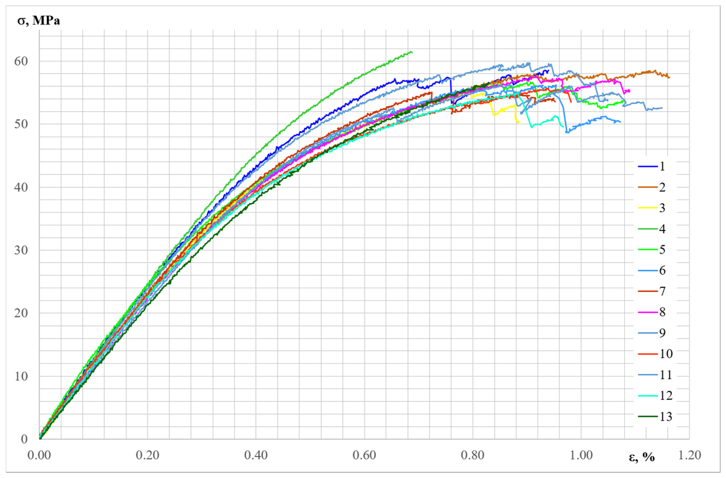
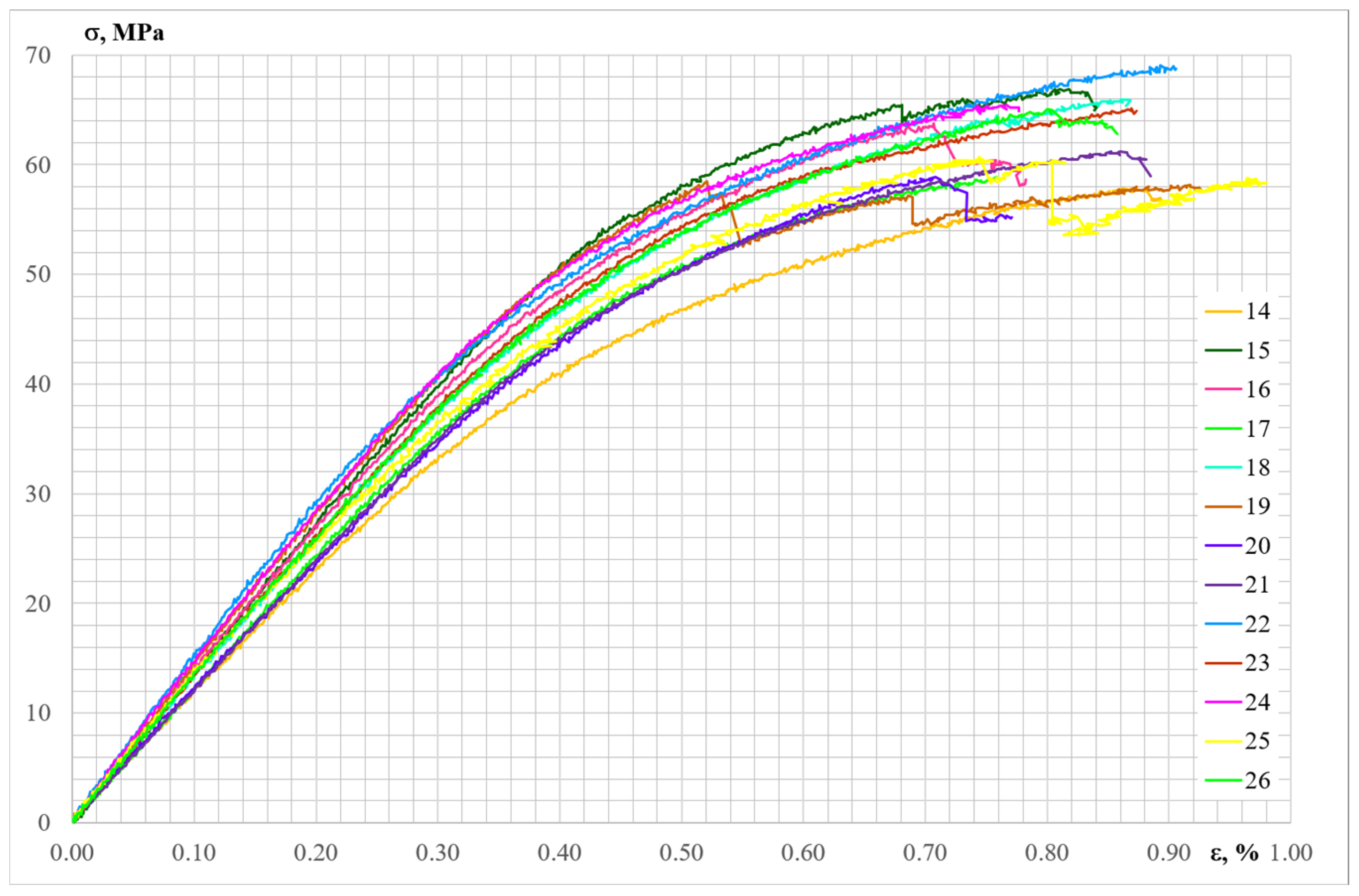
In Figure 9 and Figure 10, the stress–strain curves are presented for all tested samples.

The elastic and mechanical properties obtained from specimens 1–13 following the bending tests are presented in

Table 4. Elastic and mechanical properties determined for specimens 1–13 (Zone 2).

Specimen	E (MPa)	ν	σ (MPa)
1	11,859.329	0.610	58.521
2	11,578.626	0.499	58.512
3	11,385.623	0.582	55.055
4	12,169.887	0.594	61.505
5	12,125.934	0.596	56.702
6	11,184.350	0.581	56.224
7	11,316.363	0.490	55.042
8	11,196.819	0.556	57.470
9	12,037.897	0.527	59.767
10	11,104.735	0.525	55.614
11	10,722.823	0.508	56.367
12	11,244.853	0.559	55.033
13	10,496.330	0.633	56.509
Mean	11,417.198	0.558	57.102
Coefficient of Variation (%)	4.556	8.138	3.480

. These specimens were prepared from Zone 2 of the log.

The elastic and mechanical properties obtained from specimens 14–26 following the bending tests are presented in

Table 5. Elastic and mechanical properties determined for specimens 14–26 (Zone 1).

Specimen	E (MPa)	ν	σ (MPa)
14	11,377.891	0.391	57.902
15	13,748.768	0.237	66.919
16	13,405.529	0.401	63.763
17	12,121.346	0.402	59.205
18	12,851.169	0.350	65.935
19	14,057.679	0.494	58.478
20	11,695.921	0.424	58.858
21	11,867.011	0.438	61.167
22	14,484.817	0.466	69.030
23	12,879.824	0.444	65.094
24	14,052.997	0.390	65.455
25	12,859.135	0.440	60.696
26	13,085.641	0.453	65.021
Mean	12,960.595	0.410	62.886
Coefficient of Variation (%)	7.582	15.710	5.841

. These specimens were prepared from Zone 1 of the log.

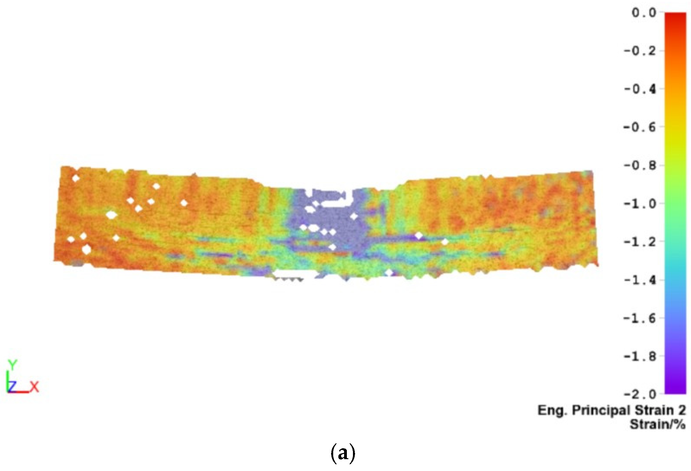
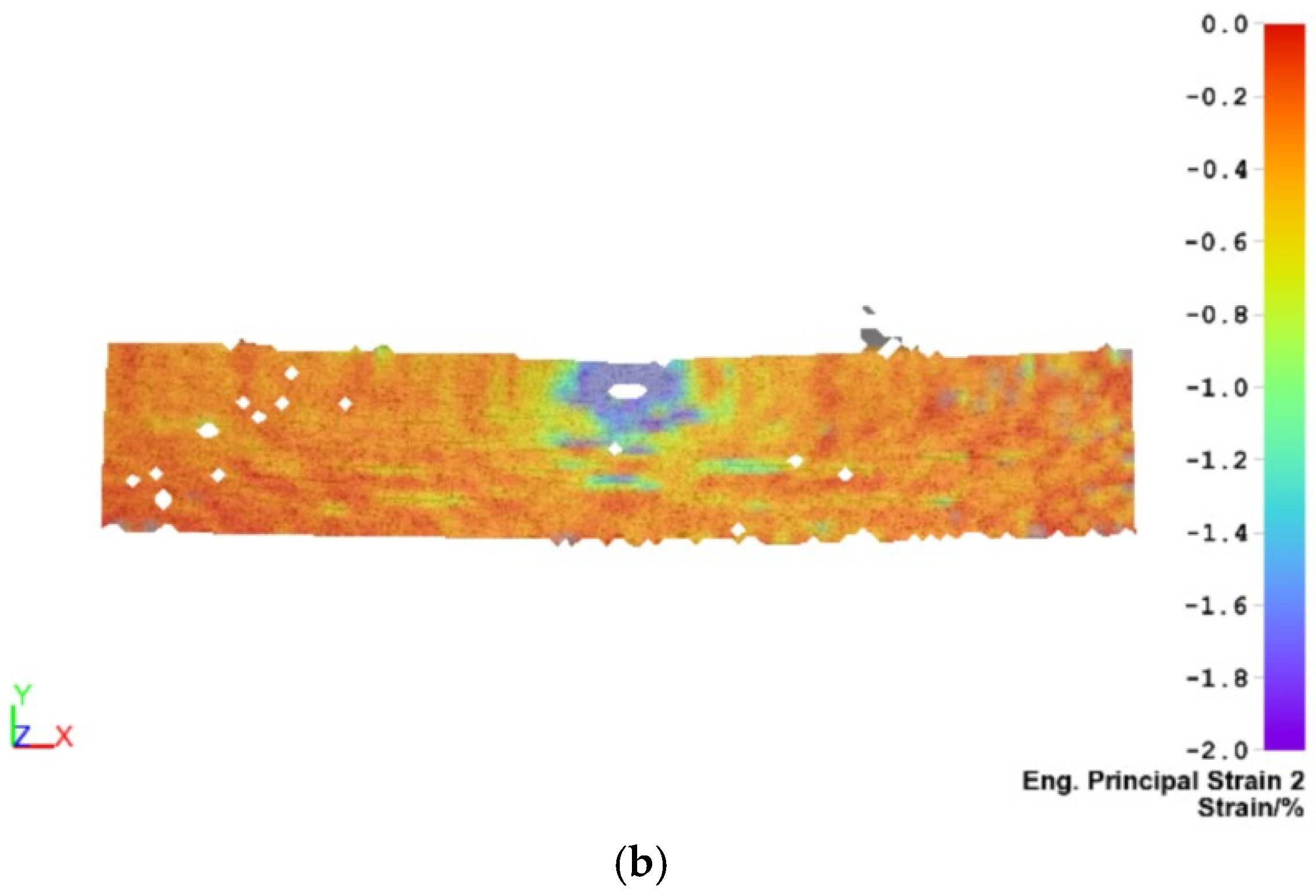
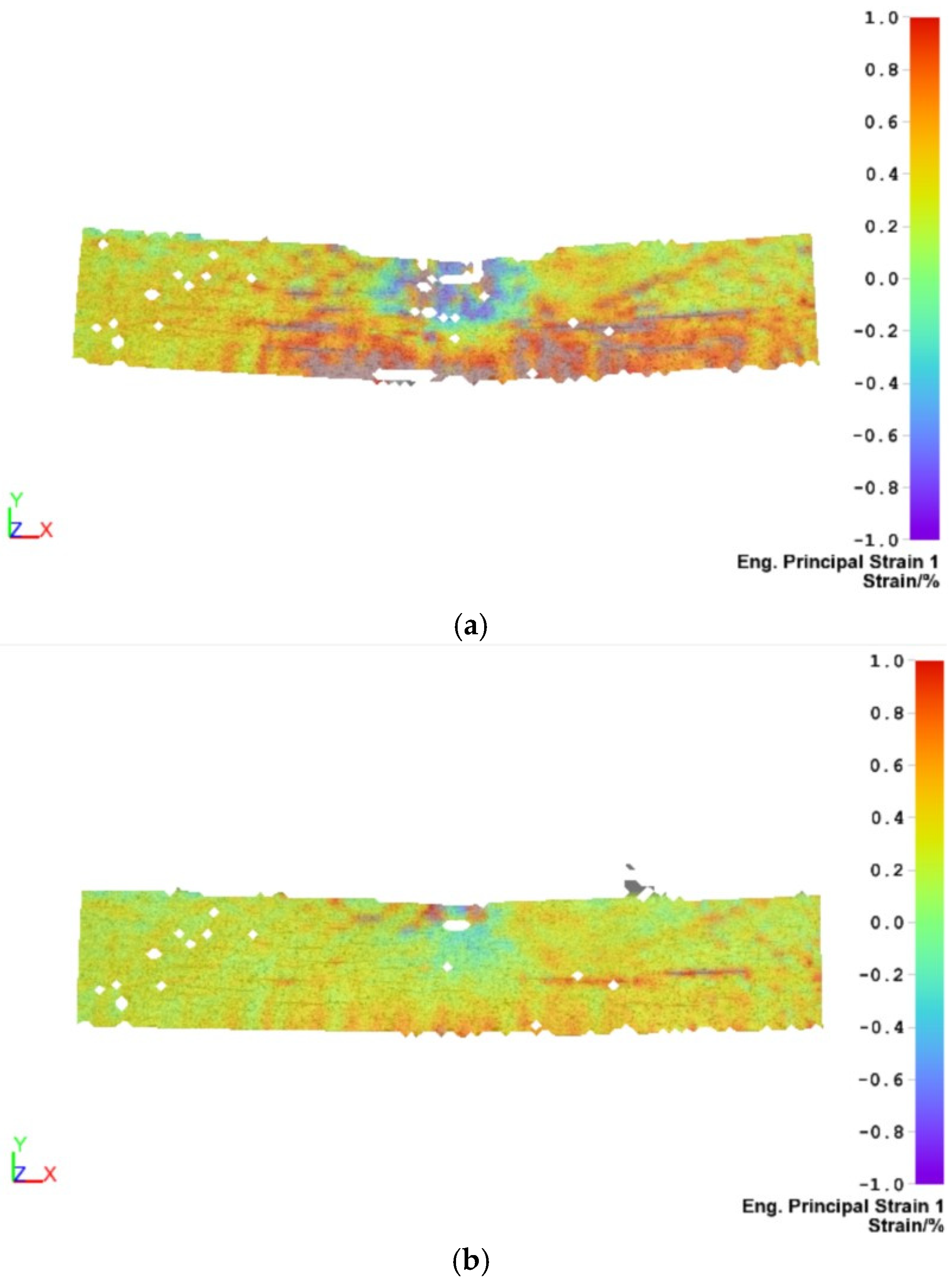
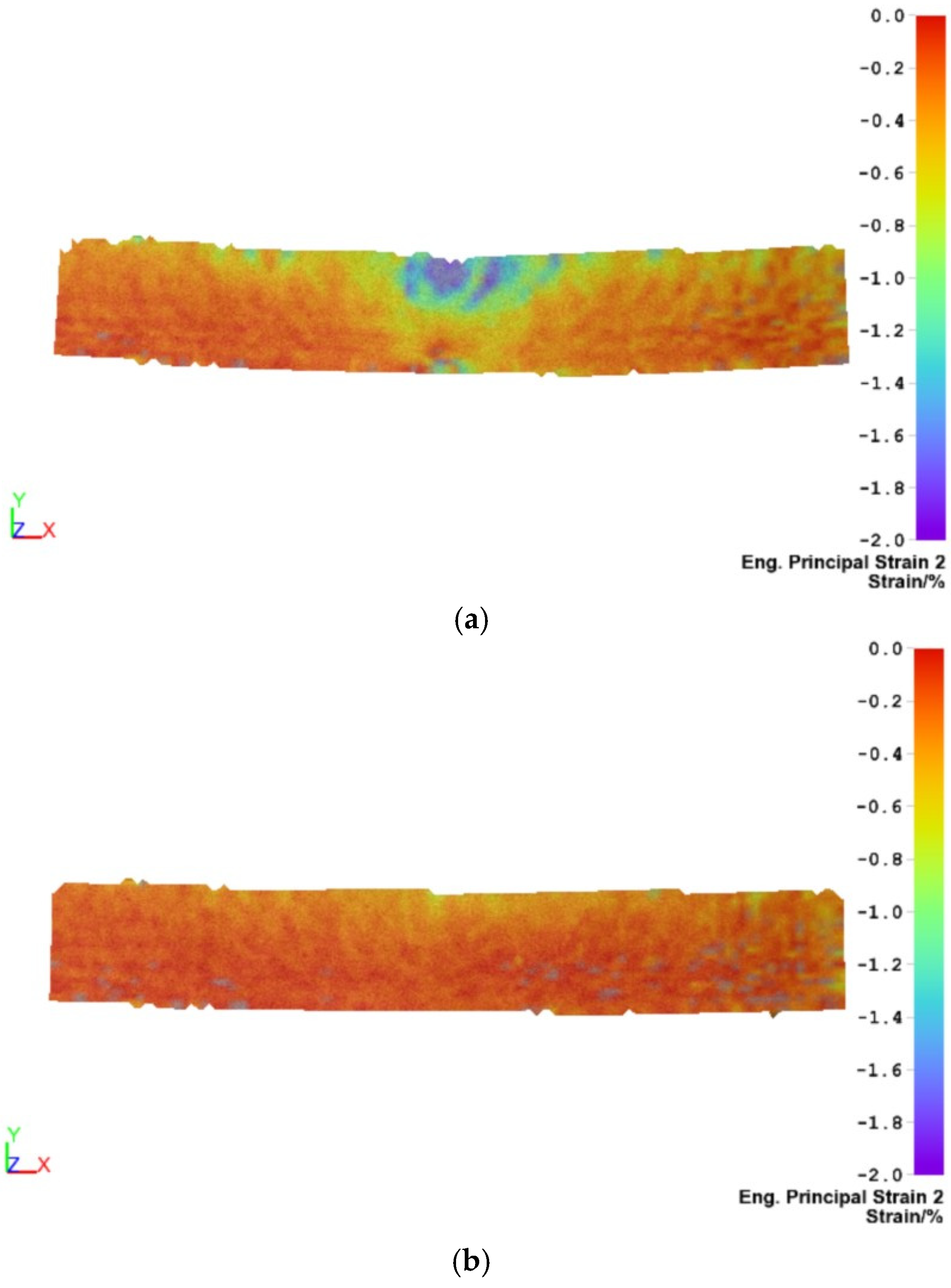
The following figures present processed images obtained using the Digital Image Correlation (DIC) system for several representative specimens selected from each test group. Figure 11 and Figure 12 show the first and second principal strain distribution for Specimen 2 (Zone 2) in the maximum stress state and in the linear region. 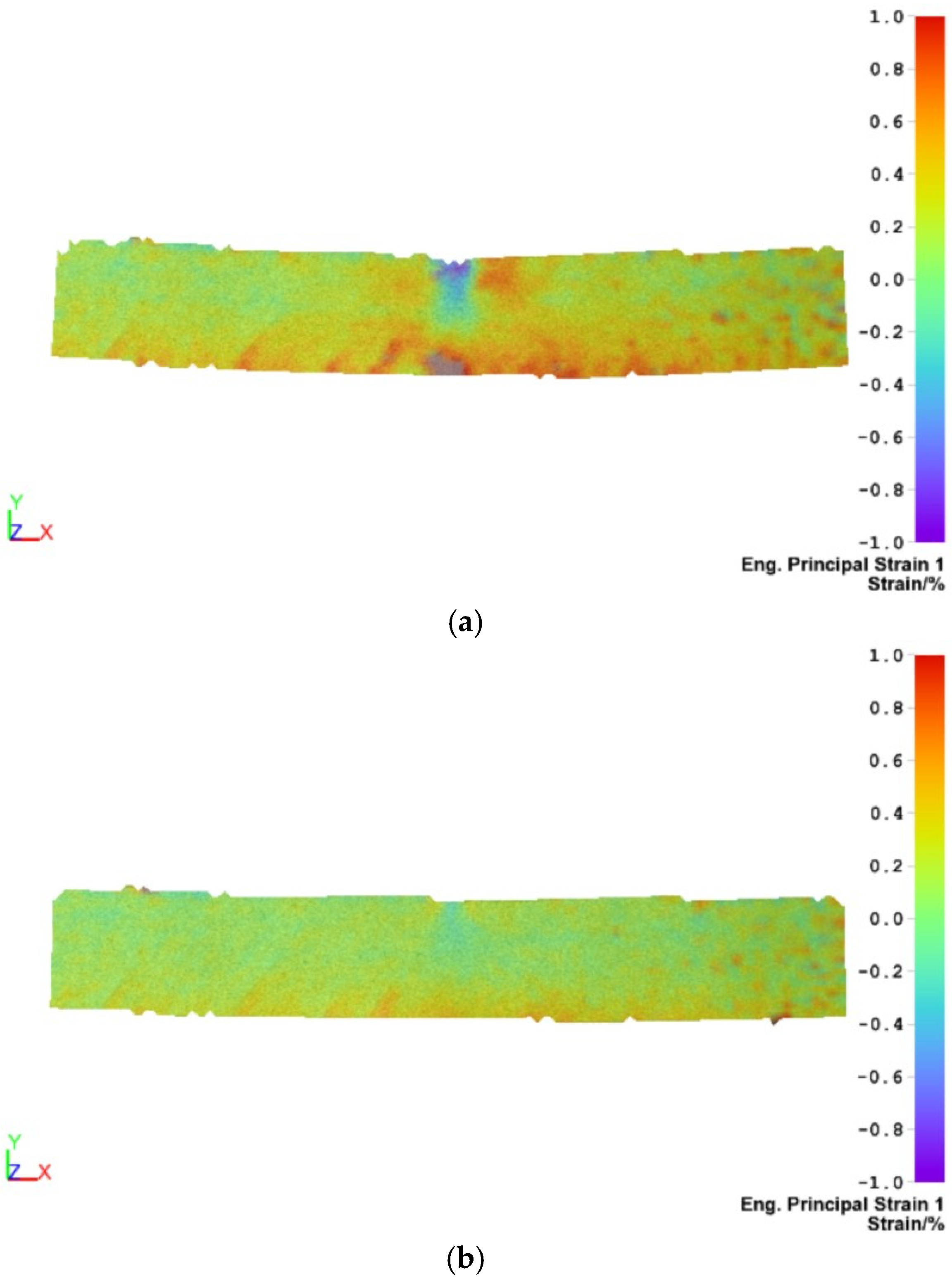The first principal strain (ε₁) corresponds to the maximum principal strain, whereas the second principal strain (ε₂) corresponds to the minimum principal strain. For each specimen, identical contour limits and color scales were adopted to enable direct comparison between different loading states.

Figure 13 and Figure 14 show the first and second principal strain distribution for Specimen 16 (Zone 1) in the maximum stress state and in the linear region.

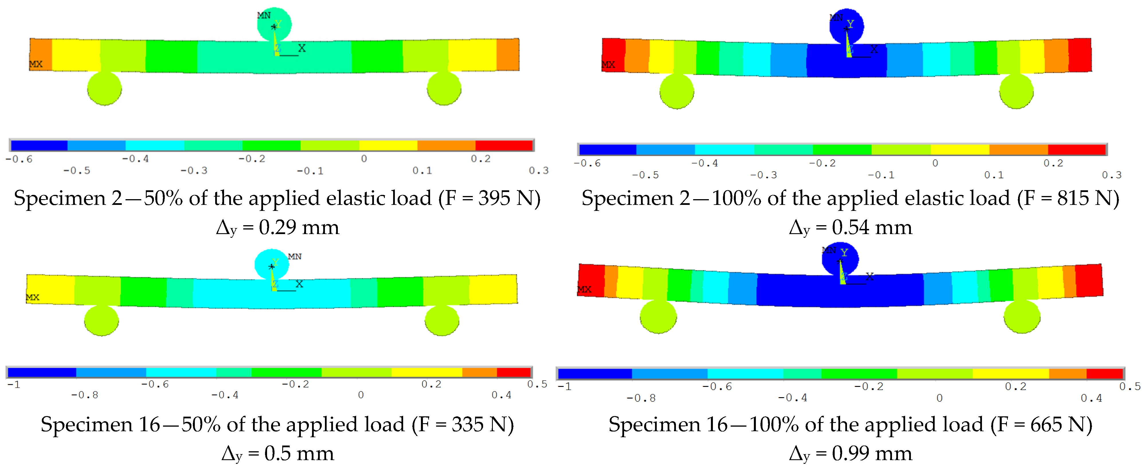
The numerically predicted directional deformation fields for the two investigated configurations are presented in Figure 15 at 50% and 100% of the elastic limit of the specimens. The contour plots represent the vertical displacement component (Δy) in the loading direction. To facilitate comparison between specimens and loading levels, all displacement maps were displayed using the same color gradient and contour limits.

The deformation patterns were consistent with the expected response of a specimen subjected to three-point bending, with the maximum vertical displacement occurring in the vicinity of the midspan section. At the maximum considered load, the highest bending displacement of 0.99 mm was achieved for specimen 16, compared with 0.5 mm for specimen 2.

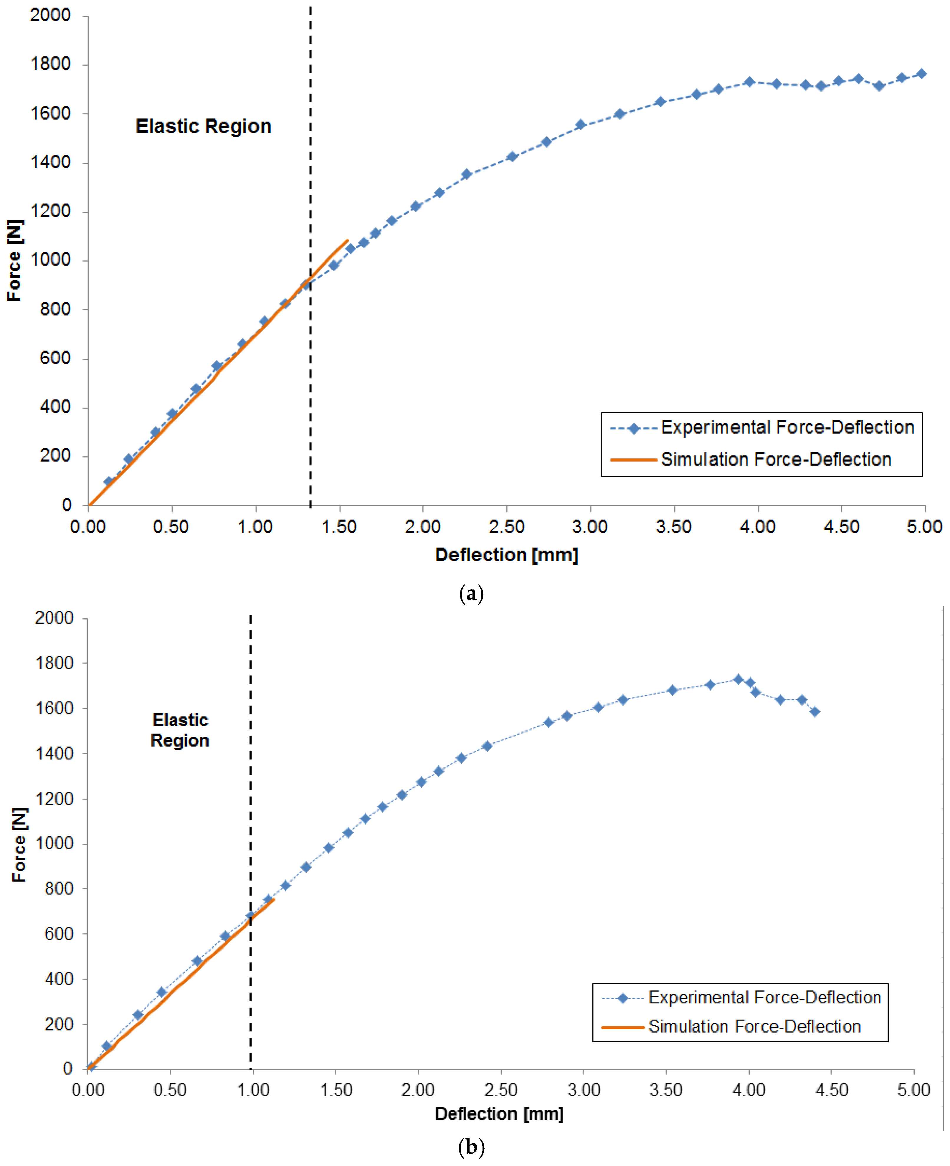
Figure 16 compares the experimentally measured and numerically predicted force–deflection curves for both investigated configurations.

In both cases, the simulation model was able to accurately recreate the behavior of the specimens in the elastic region. The maximum percentage error between the experimental and simulation curves is 3.14% for specimen 16 and 1.94% for specimen 2.

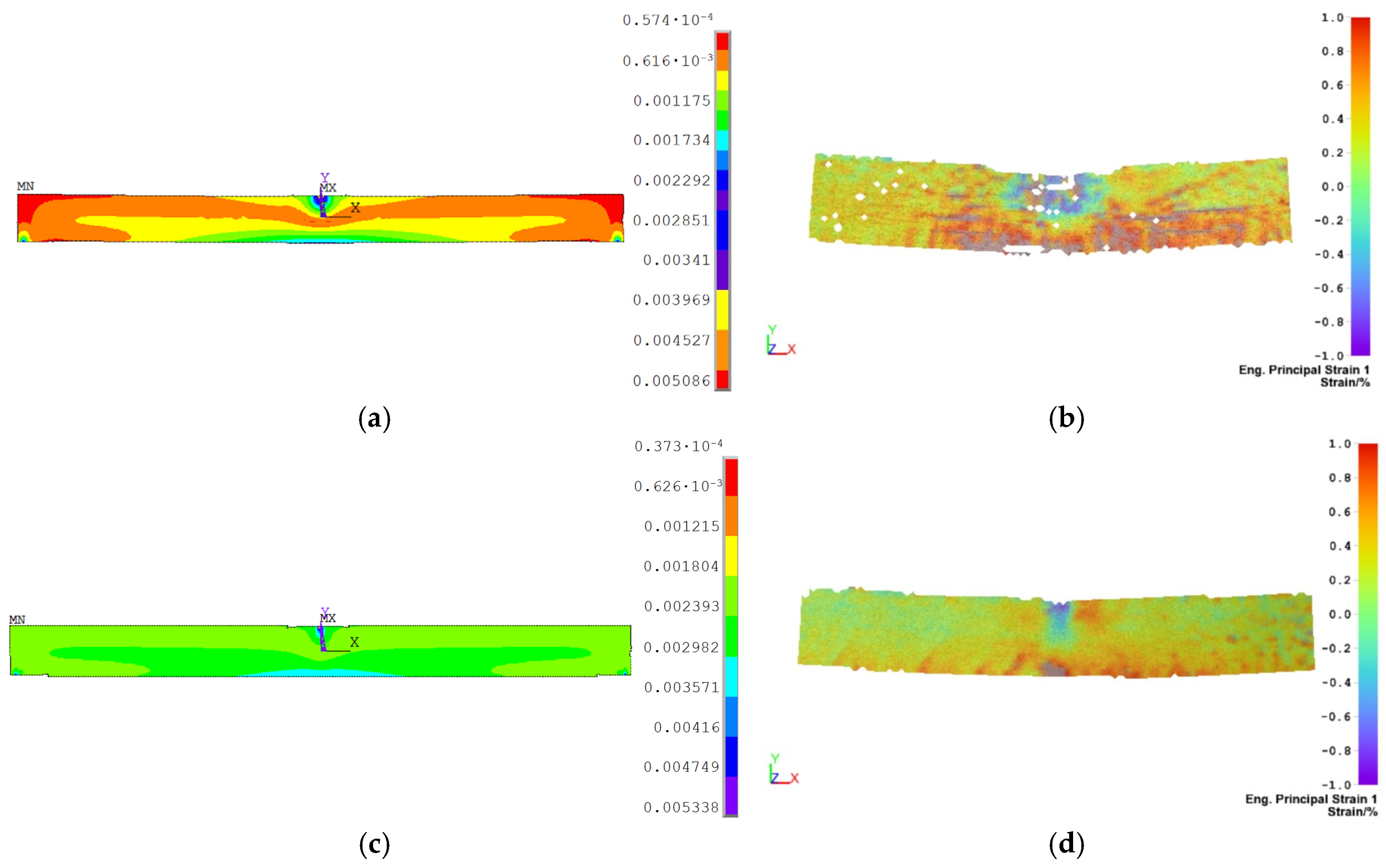
To evaluate the ability of the numerical model to reproduce the experimentally observed strain field, the first principal strain (ε₁) distributions derived from the FEM simulations were compared to the corresponding DIC measurements (Figure 17).

The comparison was conducted at 50% of the maximum elastic load for both of the investigated specimens, thus guaranteeing the response was within the predominantly elastic loading range considered by the numerical material model.

Principal strain obtained from ANSYS Mechanical APDL 19.0 (ANSYS, Inc., Canonsburg, PA, USA) was converted from its dimensionless decimal form to percentage strain to compare directly with the DIC results. In addition, the limits of the contours and the color representation of the numerical results were changed to match the experimental DIC scale.

In an effort to minimize the effect of localized numerical effects associated with the contact formulation, the FEM strain contours were limited to the region of interest corresponding to the middle span of the specimen. Element selection was carried out to remove elements outside this range and, in particular, the first row of elements adjacent to the loading and support contact interfaces. These regions showed strong local strain concentrations due to the load transfer occurring between the rigid contact edges and the wood specimen. These were omitted because it was considered that their inclusion would dominate the contour scale and obscure the strain distribution in the specimen.

For Specimen 2, five representative points along the specimen length were selected at approximately x/L = 0.20, 0.35, 0.50, 0.65 and 0.80. The points were distributed symmetrically relative to the midspan, so as to perform a consistent comparison between the FEM and DIC strain fields, obtaining the central loading region (P3) and regions progressively farther from the load application point (P1–P2 and P4–P5). This method avoids the selection of isolated local extrema and provides a more representative assessment of the spatial strain distribution.

The comparison of the five points shows a good agreement between the first principal strain values of DIC and FEM. The best agreement is seen at P3 where the FEM predicts 0.509% versus 0.50% for DIC. In the other locations, the FEM values are a little higher with absolute differences of about 0.047 to 0.053 percentage points. Both methods identify the characteristic strain variation associated with the central loading region and a comparatively more uniform response away from it, in agreement with the full-field observations reported for Specimen 2.

The increased local variations in the DIC field are related to the natural heterogeneity of wood, which is not explicitly included in the homogeneous orthotropic FEM material model. Overall, the comparison shows that the numerical model can reproduce reasonably the approximate magnitude and general spatial trend of the first principal strain observed experimentally (

Table 6. Specimen 2 comparison between FEM and DIC results.

Point	Approx. Location	FEM Principal Strain, Decimal	FEM Principal Strain, %	DIC Principal Strain, %	Approx. Absolute Difference, Percentage Points
P1	Left region, ~20% of span	0.00453	0.453	0.40	0.053
P2	Left-central region, ~35% of span	0.00397	0.397	0.35	0.047
P3	Central region, beneath/near loading point	0.00509	0.509	0.50	0.009
P4	Right-central region, ~65% of span	0.00397	0.397	0.35	0.047
P5	Right region, ~80% of span	0.00453	0.453	0.40	0.053

).

The comparison for Specimen 16 shows good overall agreement of the first principal strains between FEM and DIC (

Table 7. Specimen 16 comparison between FEM and DIC results.

Point	Approx. Location	FEM Principal Strain, Decimal	FEM Principal Strain, %	DIC Principal Strain, %	Approx. Absolute Difference, Percentage Points
P1	Left region, ~20% of span	0.00239	0.239	0.20	0.039
P2	Left-central region, ~35% of span	0.00298	0.298	0.25	0.048
P3	Central region, near loading point	0.00357	0.357	0.35	0.007
P4	Right-central region, ~65% of span	0.00298	0.298	0.25	0.048
P5	Right region, ~80% of span	0.00239	0.239	0.20	0.039

). The best agreement is in the middle region where the FEM predicts about 0.357% as compared to about 0.35% from DIC which corresponds to an absolute difference of only 0.007 percentage points. In the other regions evaluated, the FEM shows a slight overestimation of the experimental values with differences around 0.039–0.048 percentage points.

The strain distribution of Specimen 16 is observed to be more uniform over most of the middle span than that of Specimen 2, but the strain gradient is more pronounced toward the lower part of the specimen. The DIC field reveals a similar trend, where the higher strain values are mainly located toward the lower edge.

4. Discussion

The present study proposed an integrated workflow combining computer image processing, experimental testing, and finite element modelling for wood quality assessment. The classification based on YOLOv8 managed to classify specimens without defects from specimens containing visible defects, enabling an objective specimen selection process prior to mechanical characterization. Although the YOLOv8m model exhibited slightly higher detection performance than YOLOv8n, both architectures achieved comparable results and demonstrated sufficient accuracy for identifying specimens suitable for further investigation. The lower performance obtained for rare defect classes, such as brittle heart and missing knots, can be attributed to the class imbalance within the training dataset. Nevertheless, as the main objective of the computer vision was the separation of defective and defect-free wood rather than fine-grained defect categorization, both models proved suitable for the proposed application.

The automated inspection stage played a critical role in reducing the influence of natural defects on the subsequent experimental program. Using for the experimental campaign only specimens classified as defect-free, the variability associated with visible discontinuities was minimized, allowing the measured mechanical response to be more representative of the intrinsic behavior of beech wood. This finding is consistent with previous investigations that highlighted the importance of clear wood specimens when determining fundamental mechanical properties.

The results of the three-point bending tests revealed differences between the two extraction zones. Specimens obtained from Zone 1 exhibited a higher average modulus of elasticity (12,960.6 MPa) and bending strength (62.9 MPa) compared with specimens extracted from Zone 2, which exhibited average values of 11,417.2 MPa and 57.1 MPa, respectively. These differences suggest that the radial position and growth-ring orientation influence the bending response of the material. Although all specimens originated from the same log, the observed variation confirms the anisotropic and heterogeneous nature of wood and highlights the importance of controlling specimen location during sample preparation.

The Digital Image Correlation measurements provided valuable information regarding strain concentration during loading. For both chosen specimens, from both zones of the log, the highest strain values were observed in the vicinity of the loading point, where bending stresses reached their maximum values. The full-field strain maps demonstrated that deformation was not perfectly uniform throughout the specimen, reflecting the influence of local microstructural variations naturally present in wood. Nevertheless, the overall strain distributions remained consistent with the expected behavior of beams subjected to three-point bending.

The finite element simulations reproduced the experimental response with a high degree of accuracy. The force-deflection curves predicted numerically showed excellent agreement with the experimental measurements, with maximum deviations of only 1.94% for Specimen 2 and 3.14% for Specimen 16. These results indicate that the orthotropic linear-elastic material model adopted in the numerical analysis was capable of capturing the global bending behavior within the elastic region. The comparison between FEM and DIC strain fields demonstrated a good qualitative correlation. In both specimens, the numerical model correctly identified the location of maximum strains and reproduced the principal trends observed experimentally. Although the global deflection can be estimated using classical beam theory, the FEM model provides additional information on strain distribution and contact effects while enabling direct comparison with the full-field DIC measurements. Furthermore, the proposed modelling approach can be extended to more complex geometries and loading conditions where analytical solutions become insufficient.

Some differences between the numerical and experimental strain distributions were nevertheless identified. The DIC measurements revealed a more heterogeneous strain field than that predicted by the numerical simulations. This discrepancy can be explained by the simplified representation of wood as a homogeneous orthotropic material in the FE model. In reality, wood exhibits local variations in density, fiber orientation, growth-ring geometry, and microstructural features that cannot be fully captured by a continuum material model. In addition, localized experimental effects and optical measurement noise may contribute to the observed differences. Despite these limitations, the agreement achieved between the two approaches confirms the suitability of FEM as a complementary tool for predicting the mechanical behavior of defect-free beech wood.

Overall, the proposed methodology establishes a direct connection between automated defect detection and structural characterization. The YOLOv8 models ensured consistent specimen selection, while the combination of three-point bending tests, DIC measurements, and finite element simulations provided a comprehensive understanding of the mechanical response of the selected material. This study may support future developments in automated wood grading systems, where artificial intelligence-based inspection can be integrated with mechanical performance assessment to improve reliability and reduce the subjectivity associated with traditional visual evaluation procedures.

The value of the proposed methodology lies in the complementary information provided by each technique and in establishing a validated link between automated defect screening and mechanical characterization of wood. Three-point bending tests supply the global mechanical response, DIC provides full-field strain measurements, and FEM enables the interpretation of these results through a numerical representation that accounts for orthotropic material behavior and contact interactions. The defect-free configuration investigated in this study serves as a controlled baseline for the integrated framework. The results demonstrate that AI-based specimen selection can reduce the influence of visible defects and support a reliable correlation between experimental measurements and numerical predictions. Future developments may incorporate image-derived defect geometry and location into specimen-specific FEM models, enabling more realistic analyses of the local mechanical effects of knots and other defects under complex loading conditions.

5. Conclusions

This study demonstrated the feasibility of integrating artificial intelligence, experimental testing, and numerical modelling for wood quality assessment.

The main conclusions are as follows:

• The YOLOv8-based framework provided reliable identification of defect-free wood specimens, supporting automated and objective specimen selection for subsequent analyses.
• The use of AI-based screening prior to testing reduced the influence of visible defects and contributed to the good agreement observed between the experimental measurements and FEM predictions.
• Three-point bending tests revealed differences between specimens extracted from the two investigated log zones, suggesting an influence of growth-ring orientation and sampling location on the measured mechanical properties of beech wood.
• The combination of DIC and FEM enabled a quantitative comparison between experimentally measured and numerically predicted strain fields, confirming the ability of the numerical model to reproduce the deformation behavior of defect-free beech specimens.
• The finite element model accurately reproduced the experimental response, with errors below 3.2%, demonstrating the suitability of an orthotropic elastic material model for predicting the bending behavior of defect-free beech wood.

Overall, the proposed workflow establishes a practical link between automated defect detection and structural assessment, supporting the development of more reliable wood grading and quality evaluation methodologies.