Article

A Time-Resolved Analysis of VOCs and VVOCs from Interior Wood Materials in Low-Ventilation Environments


by
Shahla Ghaffari Jabbari
1,*,
Jose Fermoso Domínguez
2,
Sandra Rodríguez Sufuentes
2,
Svein Olav Nyberg
1,
Tore Sandnes Vehus
1 and
Henrik Kofoed Nielsen
1
1
Department of Engineering Sciences, University of Agder (UiA), Jon Lilletunsvei 9, 4879 Grimstad, Norway
2
CARTIF Technology Center, Parque Tecnológico de Boecillo, Parcela 205, 47151 Boecillo, Valladolid, Spain
*
Author to whom correspondence should be addressed.
Forests 2026, 17(8), 884; https://doi.org/10.3390/f17080884
Submission received: 22 May 2026 / Revised: 20 July 2026 / Accepted: 27 July 2026 / Published: 29 July 2026
(This article belongs to the Section Wood Science and Forest Products)

Abstract

Selecting interior wood materials requires balancing functional and aesthetic demands with indoor air quality, as wood can emit volatile organic compounds (VOCs) and very volatile organic compounds (VVOCs) that either peak shortly after installation or persist over time. This study investigated time-resolved VOC and VVOC accumulation concentrations from untreated pine, spruce, aspen, and oak, representing wood species commonly used in Norway. Concentrations of VOCs and VVOCs were monitored for 25–28 days under low-ventilation, worst-case chamber conditions using Proton Transfer Reaction–Time-of-Flight Mass Spectrometry (PTR-TOF-MS). Emission behaviour was assessed using peak concentration, decay rate, half-time, stabilised concentration, cumulative exposure (AUC28), and available health-based thresholds. Clear species-dependent differences were observed. Pine was the dominant VOC source, with the highest peak concentration, stabilised concentration, and AUC28, mainly due to monoterpenes, which remained above the health-based threshold throughout the test period. Oak showed the second-highest VOC burden and a distinct acetate-dominated profile, with acetic acid showing the longest predicted exceedance duration. Aspen and spruce had lower VOC burdens, but their cumulative VVOC exposure exceeded VOC exposure. VVOCs generally peaked earlier than VOCs, although persistence varied by species. Overall, the concentration of VOCs and VVOCs was controlled by species, compound chemistry, volatility, and internal transport, supporting species- and compound-specific ventilation and material-selection strategies.

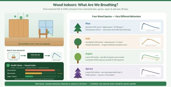
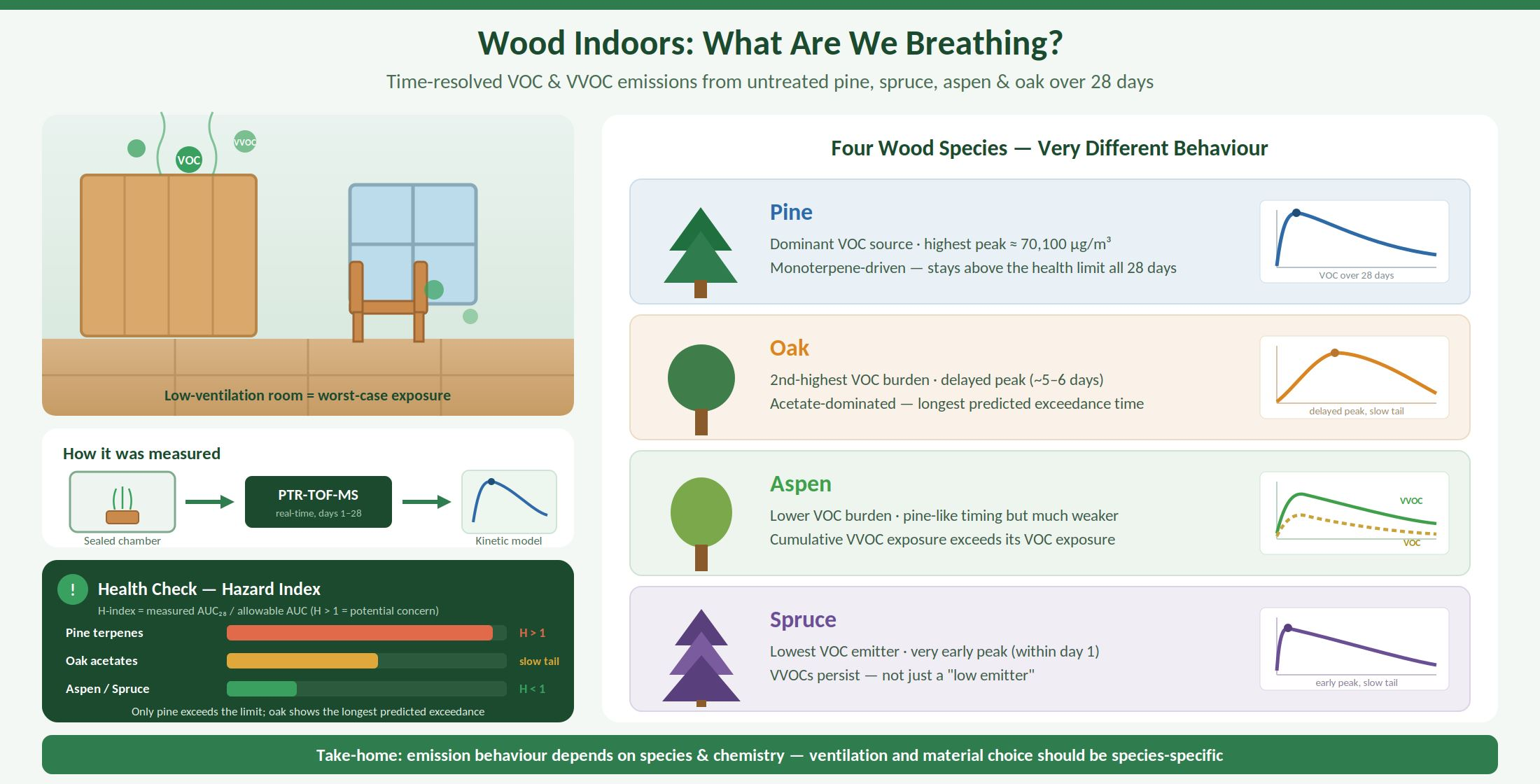
Graphical Abstract

1. Introduction

Building materials are among the primary sources of volatile organic compound (VOC) emissions, which can significantly influence the chemical composition of indoor air [1]. These emissions vary depending on the type of material, its physical and chemical properties, and environmental conditions [2]. Shao [3] demonstrated that pore geometry, porosity, and fractal characteristics strongly influence the diffusion and release of VOCs. VOC emission behaviour is also governed by diffusion and sorption processes within the material matrix, which determine both source and sink dynamics over time [4].
Volatile organic compounds (VOCs) are known to cause various acute negative health effects, such as headaches, dizziness, and sensory irritation. Chronic exposure to VOCs can lead to more serious health issues like respiratory diseases and even cancer [5]. Several studies discussed the long-term and short-term health issues due to exposure to different VOCs [6,7,8]. Time behaviour of VOCs, referring to when and how much these compounds are released over time, is a critical factor in their health impact, primarily by influencing secondary pollutant formation and exposure timing [9,10], both of which are linked to adverse health outcomes.
Different compounds exhibit considerable variation in their emission timeline depending on the source, such as building materials, temperature, and compound properties. Some VOCs are released rapidly, while others persist from building materials and contents, leading to ongoing exposure over time [11,12], thereby influencing cumulative exposure through extended tail emissions. Recent studies in building physics have highlighted the importance of conjugate mass transfer in explaining these temporal differences, linking the diffusion coefficient and partitioning behaviour of VOCs to their measured emission tails [4].
Key physicochemical properties, notably volatility and polarity, determine whether a compound emits a high-intensity initial burst or a prolonged, diffusion-limited emission tail [13,14]. These kinetic distinctions become particularly significant in environments with low ventilation, since the volatiles are potentially exposing occupants to brief emission peaks soon after installation, while the background levels may prevail over the long-term exposure. Among building materials, wood is extensively utilised in indoor settings in wall, ceiling panels, furniture, shelving, and flooring, and is increasingly endorsed for its environmental and aesthetic advantages. This widespread usage necessitates prioritising the wood–indoor air interface within exposure science.
Although numerous studies have identified primary compounds emitted from wood and recorded concentrations at specific time intervals [15,16,17], far fewer have assessed the rate at which various chemical classes reach peak levels, decay, and maintain measurable baselines from interior products, especially under static, low-ventilated conditions that simulate worst-case indoor environments. Additionally, existing time-resolved studies on VOC emitted by wood products have frequently been restricted to a narrow set of marker analytes or have generalised emissions as total VOC (TVOC), rather than resolving class- or compound-specific kinetics [18,19]. Parallel work on non-wood materials, notably interior paints/varnishes, coatings, and adhesives, has documented rapid early maxima followed by first-order or bi-exponential decline, with clear substrate and film-thickness effects that modulate evaporation versus diffusion-controlled tails [20,21]. Pertinent questions remain unanswered regarding exposure and wood interior product selection: Which chemical groups dominate the initial peak as opposed to the extended tail? How do emission half-lives and baseline plateaus vary between species? Which compounds have the most significant impact on cumulative exposure during occupancy periods?
To address these uncertainties, this study quantified time-resolved emissions from four commonly used interior wood types, including pine, spruce, oak and aspen over 28 days using proton-transfer-reaction time-of-flight mass spectrometry (PTR-TOF-MS). The study aimed to explore the time-dependent accumulation and persistence of VOCs emitted from common indoor wood materials under static, low-ventilated conditions and to quantify and compare the short- and long-term emission behaviours of VOCs and VVOCs across four untreated wood species.

2. Materials and Methods

A detailed analysis of VOC and VVOC emission time behaviours was conducted for four commercially available wood interior panels from a Norwegian market, including untreated species of fresh pine (Pinus sylvestris), aspen (Populus tremula), oak (Quercus robur), and spruce (Picea abies), using a Proton Transfer Reaction–Time of Flight–Mass Spectrometry (PTR-TOF-MS 1000, Ionicon Analytik, Eduard-Bodem-Gasse 3, 6020 Innsbruck, Austria, RRID: SCR_026459). Wood panels were sourced from Bergene Holm AS and were manufactured in Norway. These species were chosen due to their widespread use and relevance for interior applications in Norway. All samples were produced from heartwood, cut to dimensions of 70 × 70 mm, and prepared to expose only the intended surface for emission testing, with all other faces sealed using emission-free aluminium tape. Sample preparation, selection rationale, and measurement protocols are described in detail elsewhere [22]. Accumulated VOC and VVOC concentrations were measured over approximately 28 days. Measurements were performed at nominal time points of days 1, 3, 7, 10, and 14 for all samples. Due to practical laboratory and PTR-TOF-MS scheduling constraints during the final sampling period, the final measurement could not be performed on the same day for all species. Final measurements were conducted on day 25 for aspen (Populus tremula) and oak (Quercus robur), while pine (Pinus sylvestris) and spruce (Picea abies) were monitored until day 28. Consequently, individual samples were followed for 25–28 days, and modelling was performed using the actual measurement times for each species.
The samples were carefully prepared, stored, and analysed under controlled conditions to minimise variability and potential contamination. Each wood sample was enclosed in a sealed 0.98 L glass chamber set within a 1 m3 climate-controlled environment at 25 ± 1 °C and 50 ± 5% relative humidity, without active ventilation, with a controlled loading rate of 5 m2/m3, based on the sample area and chamber volume.
Although the bottles were operated without active ventilation, PTR-TOF-MS sampling introduced a small effective air exchange. Based on a sampling flow of 80 ± 20 mL/min for 3 min and a bottle volume of 0.98 L, each measurement corresponded to approximately 0.24 ± 0.06 air changes per event. Across the full experiment, this resulted in a cumulative exchange of approximately 1.4 ± 0.4 air changes over the 28-day monitoring period, confirming that the setup represented a quasi-static, worst-case low-ventilation condition. PTR-TOF-MS signals were processed using the Ionicon PTR-TOF Data Analyser and reported as volume mixing ratios in ppb or ppb-equivalent units after normalization of ion signals, mass-axis calibration, and transmission correction. An external acetone standard was used for instrument calibration. Since authentic standards were not available for all detected compounds, compound-specific response factors could not be determined for the full mass spectrum. Therefore, concentrations for compounds other than acetone should be interpreted as semi-quantitative values expressed relative to the acetone calibration and the PTR-TOF-MS response model. The ppb or ppb-equivalent values were subsequently converted to µg/m3 using the molecular weight of the tentatively assigned compound or elemental formula. Concentrations were divided by the test loading rate to obtain loading-normalised values, allowing comparison with the EN 16516 reference-room wall loading of 1.0 m2/m3 [23]. Accumulated VOC and VVOC concentrations from the samples were continuously monitored using the PTR-TOF-MS system. To verify the accuracy and reliability of our VOC measurements, the experimental setup included background correction via two blank chambers (one empty and one containing aluminium tape), which was subtracted from the corresponding sample measurements to ensure that signals primarily reflected emissions from the wood samples. Each species was tested in duplicate (two replicate bottles per material). Figure 1 illustrates the experiment setup for time-resolved VOC and VVOC headspace measurements from wood samples under quasi-static low-ventilation conditions.
PTR-TOF-MS signals were categorised into Very Volatile Organic Compound (VVOC) and Volatile Organic Compound (VOC) groups according to the volatility ranges defined in EN 16516, based on tentative assignments supported by exact mass and library information. This classification enabled a nuanced evaluation of the emission profiles of different wood types, supporting broader insights into indoor air quality implications and material selection. Since PTR-TOF-MS does not provide chromatographic separation, this classification was not intended as definitive molecular identification, but as a screening-level ion- and compound-family-based approach. PTR-TOF-MS was selected because the aim of the study was not to quantify only a predefined set of target molecules, but to capture a broader time-resolved profile of emitted ion signals across the VOC and VVOC ranges.
Following the acquisition of time-resolved VOC and VVOC concentrations for each of the four wood species, bulk-TVOC and bulk-TVVOC decay profiles were first modelled using a bi-exponential function to differentiate early-peak and extended-tail chemistries across VVOCs and VOCs. From these fits, peak emission times (tmax), decay constants (a, b), half-life (t1/2), and baseline concentrations (C) were determined for each sample.
Kinetic parameters were then fitted to material properties (surface desorption versus internal diffusion), resulting in interpretable metrics for improved design and ventilation strategies in environments with low air exchange. Finally, the kinetics were linked to exposure relevance through Area-Under-Curve (AUC) and compared with allowable exposure limits derived from health-based indoor air quality thresholds (e.g., Lowest Concentration of Interest, LCI; Threshold Limit Value–Time-Weighted Average, TLV-TWA), adjusted for continuous exposure conditions. The hazard index (H-index) was computed as the ratio of measured to allowable AUC, with values greater than unity indicating a potential for sensory irritation or other non-cancer effects under prolonged indoor exposure.
This ion- and compound-family-level analysis enabled the identification of the main VOC and VVOC signals contributing to emission kinetics and potential exposure relevance. Where suitable tentative assignments and health-based reference values were available, the fitted profiles were used to estimate the time required for selected VOC groups to decline below reference levels. This provides a basis for future confirmatory studies and supports wood-product selection and ventilation strategies aimed at reducing occupant exposure. In particular, the approach moves beyond static concentration snapshots by providing a time-resolved, class-level assessment of wood concentrations during the first month after installation.

2.1. PTR-TOF-MS and Ion Fragmentation Correction Protocol

PTR-TOF-MS 1000 was operated under standard conditions (drift tube: 80 °C, 3.00 mbar, 720 V), with a sampling flow rate of 60–100 mL/min through the bottle inlet for 3 min. Instrument calibration employed a single-point acetone standard via the Ionicon Liquid Calibration Unit (LCU). The mass axis was verified against H3O+ (m/z 19.018) and protonated acetone (m/z 59.049), with in-line recalibration using naturally emitted decanal (m/z 157.150) and acetaldehyde (m/z 45.034). The resulting mass drift was ≤±3 ppm, meeting the Aerosol, Clouds, and Trace Gases Research Infrastructure (ACTRIS) PTR-MS accuracy requirements by [24,25]. Consequently, the factory transmission function was applied without additional user-derived corrections. All raw data were processed with the Ionicon PTR-TOF Data Analyser (RRID: SCR_026458), which automatically compensates for sampling-duty variations across the m/z axis [26].
In PTR-TOF-MS, the high mass accuracy and time-of-flight exact-mass information can support formula-level ion assignment and can distinguish many ions with different elemental compositions that overlap at nominal mass [27]. However, exact mass alone does not provide structure-level confirmation. Therefore, compound assignments in this study were considered tentative and were interpreted at the ion, elemental-formula, or compound-family level rather than as definitive molecular identifications.
Tentative compound assignments followed the GLOVOCS library [28]; peaks with <±0.05 Da difference in their m/z values were excluded, as recommended by [29]. Instrument calibration, mass-axis stability checks, raw-data processing, and tentative peak assignment followed the procedures described by [25,26,27,28].
For ion fragmentation correction, the current ACTRIS PTR-MS guidelines distinguish two acceptable ways [30]: (i) direct summation of parent and interference-free fragment ions, which propagates an expanded uncertainty of ≈30% [31,32], and (ii) application of an empirical yield factor (IF) to the parent ion alone when the fragment mass is obscured; because IF varies with humidity and reduced electric field (E/N), its use typically carries ≈50% uncertainty [33,34]. Yield factors reported for monoterpenes vary widely: 0.22–0.28 in a clean-tube study [35]; 0.25 ± 0.05 in a mixed-standard test [36]; and a field-derived 0.60 ± 0.05 for Scots-pine emissions [34]. This 0.2–0.6 spread reflects genuine sensitivity to instrument settings and VOC mix. Due to calibrating the PTR-TOF-MS only with an external acetone standard, compound-specific response factors were unavailable for the rest of the spectrum. Therefore, all concentrations were semi-quantitative and expressed relative to the acetone calibration.
Following ACTRIS PTR-MS QA/QC guidance and the VOC/VVOC definitions in EN 16516 [23], mass peaks were classified into VOC or VVOC classes only when the parent ion or compound family could be tentatively assigned with sufficient confidence. Peaks with ambiguous or overlapping assignments, for example, signals occurring within ±0.05 Da of multiple possible candidates, were excluded from compound-specific and compound-family interpretation to reduce the risk of misclassification. For compounds or compound families with well-documented parent–fragment patterns, such as isoprene (m/z 69 + 41) and monoterpenes (m/z 137 + 67 + 81 + 95), a direct summation approach was applied, whereby parent and fragment ion intensities were combined to estimate the bulk contribution of the corresponding compound family. An expanded uncertainty of approximately ±30% was applied to these sums, consistent with published recommendations for direct-summation protocols [30,32,37,38]. For the C7H8-related aromatic signal, the ion was tentatively assigned to toluene based on exact mass, library information, and the common PTR-MS interpretation of protonated toluene as C7H9+ at m/z 93. Previous PTR-MS and chromatographic comparison studies have reported good agreement for toluene measurements, including under conditions with enhanced monoterpene loading, supporting the use of m/z 93 as a reasonable toluene-related marker when interpreted cautiously [36,39]. However, exact mass alone cannot distinguish toluene from exact-mass-identical C7H8 isomers, such as cycloheptatriene, norbornadiene, or quadricyclane, nor can it fully exclude possible contributions from aromatic fragments or monoterpene-related fragmentation at m/z 93. Therefore, these possible contributions were not assigned or quantified separately. Instead, the signal was retained in the compound-specific discussion only as a C7H8-related aromatic compound tentatively assigned to toluene. Bulk TVOC and TVVOC were calculated as the sum of all detected ions within the respective VOC/VVOC ranges and were used only for overall kinetic comparison, not for definitive compound-specific identification or health-based interpretation.

2.2. Data Analyses

The dataset [40] was analysed using Python (Version 3.11) [41]. Time-dependent chamber VOC concentrations were fitted by nonlinear regression using an offset bi-exponential model (Equation (1)). This form was selected because the chamber profiles exhibited an early rise to a maximum followed by a slower decline. The selected equation is consistent with the difference-of-two-exponentials structure of ventilated chamber source models and with previous chamber studies that used multi-exponential equations for VOC-emitting materials [42,43,44].
Ct = Ae−at − Be−bt + Cbaseline [µg/m3]
where Ct represents the late-time asymptotic concentration, while A and B are amplitude parameters that control the contribution of the two exponential terms. The term Ae−at describes the slower declining component of the concentration profile, where a [d−1] is the effective decay rate constant. The term Be−bt describes the faster early-time component associated with the initial build-up towards the observed maximum, where b [d−1] is the effective rate constant. From the fitted curves, peak time, peak concentration, Area Under Curve (AUC28), half-time, and the goodness of fit (R2) were calculated to compare the emission behaviour among samples. The half-time of this component was calculated as t1/2 = ln(2)/a [day] [42]. This approach is in agreement with previous studies that attribute early-time peaks to rapid desorption from exposed microstructures and the subsequent slow decline to diffusion-limited depletion of a finite VOC reservoir material [42,43]. The cumulative exposure over the 28-day period was expressed as the area under the concentration-time curve (AUC) derived from the fitted bi-exponential model (Equation (2)).
AUC = ∫0t Ct dt [mg × d/m3]
To evaluate the potential health risks associated with prolonged exposure to the dominant emitted VOCs and VVOCs, the 28-day area under the concentration–time curve, AUC28, was calculated for each compound and compared with compound-specific allowable cumulative exposure values. These allowable values were derived from the 8-h Threshold Limit Value–Time-Weighted Average (TLV-TWA) [45]. According to the ACGIH, a TLV-TWA represents the average airborne concentration of a substance to which nearly all workers may be repeatedly exposed, day after day, for an 8-h workday and a 40-h workweek, without adverse health effects over a working lifetime. To extrapolate the TLV-TWA from an 8-h occupational scenario to continuous exposure over 24 h per day, 7 days per week, the Brief and Scala model was applied (Equation (3)) as recommended by the Canadian Centre for Occupational Health and Safety [46].
Cguide = TLV × (40/hours worked per week) × ((168 − hours worked per week)/128) [mg/m3]
In accordance with Haber’s law, the allowable cumulative exposure over a 28-day period was calculated as [47]:
AUCallowable = Cguide × t [mg·d/m3]
The hazard index (H-index) was then computed as H = AUCnorm/AUCallowable. An H-index greater than unity indicates that the cumulative exposure exceeds the allowable threshold, suggesting a potential health risk under long-term exposure conditions.

3. Results and Discussion

3.1. VOC Concentration Across Wood Samples

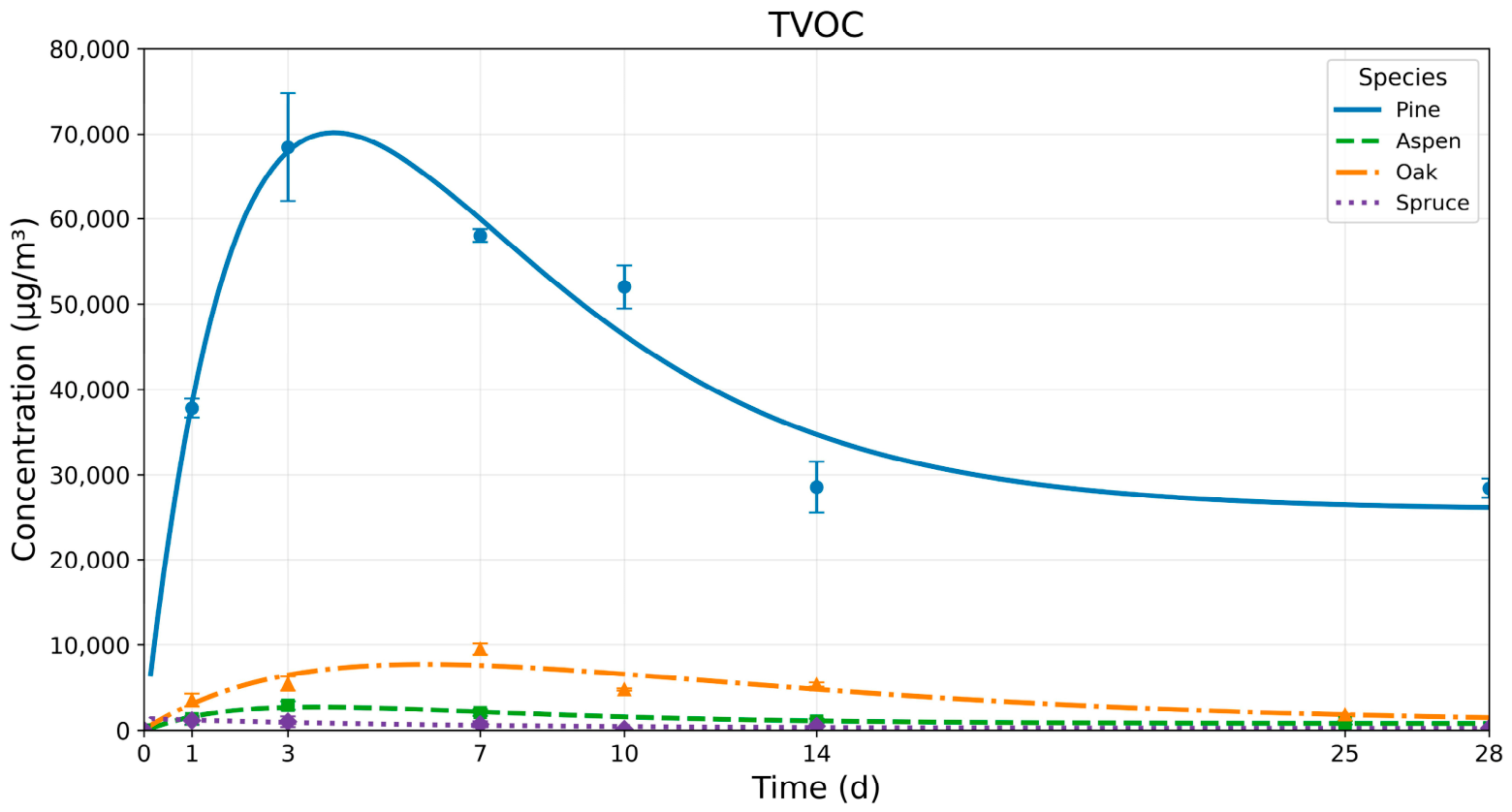
Figure 2 shows the total VOC accumulated concentration measured from the examined wood samples. Table 1 summarises the corresponding fitted parameters. Clear differences were observed among the wood species in terms of peak concentration, concentration decay, stabilisation level, and cumulative 28-day exposure. Overall, pine showed the highest total VOC concentration, followed by oak, while aspen and spruce emitted substantially lower concentrations. This species-dependent behaviour is consistent with previous studies showing that VOC concentrations from wood are strongly governed by wood species, extractive composition, anatomical structure, and processing history [17,48,49]. Among the investigated species, pine showed the highest VOC emission intensity throughout the experiment.
The concentration reached a maximum of 70,100 ± 3500 µg/m3 after 3–4 days. This was followed by a gradual decay, characterised by a decay constant of 0.3 ± 0.04 d−1 and a half-time of 2.3 ± 0.02 days. By the end of the experiment, pine stabilised at a relatively high concentration of 25,800 ± 1590 µg/m3.
The initial increase followed by a decline can be explained by a dynamic mass balance between VOC release from the wood, sorption to chamber surfaces, re-partitioning between the headspace and wood surface, depletion of the readily available VOC reservoir, and the small air exchange introduced during PTR-TOF-MS sampling. During the initial phase, the VOC release rate from surface and near-surface wood reservoirs exceeded removal and retention processes, resulting in an increase in headspace concentration. After the maximum concentration was reached, the readily releasable VOC fraction became depleted, and the system moved towards wood–air/chamber equilibrium. At this stage, chamber-wall adsorption, re-adsorption or partitioning back to the wood surface, and minor sampling-induced dilution may have exceeded the continuing release from the wood, causing the observed decline in net headspace concentration. This interpretation is consistent with diffusion–sorption-controlled VOC behaviour in porous building materials [50,51,52] and explains why a peak followed by a decline can occur even under low-ventilation conditions. The reproducible initial increase over several days also suggests that leakage was unlikely to be the dominant mechanism, because dominant leakage would be expected to suppress sustained accumulation from the beginning of the test rather than allow species-specific maxima to develop.
Pine also had the highest cumulative 28-day exposure, confirming that it was the dominant VOC source among the tested species. This behaviour is consistent with the known high terpene content of pine, particularly in resin ducts and extractive-rich tissues, which can act as reservoirs for prolonged VOC release [16,49].
Aspen showed a temporal pattern similar to pine, with a comparable decay constant of 0.3 ± 0.01 d−1 and half-time of 2.2 ± 0.08 days. Its maximum concentration occurred at 3.6 ± 0.1 days, close to the peak time observed for pine. However, the concentration magnitude was much lower. Aspen reached a peak concentration of 2747 ± 450 µg/m3, which was approximately 25 times lower than pine. Its stabilised concentration was also low, at 778 ± 215 µg/m3. This indicates that, although aspen followed a similar time-dependent release pattern, its source strength was much weaker. The lower VOC burden from aspen is consistent with the generally lower terpene reservoir in hardwoods compared with resin-rich conifers, although some hardwoods may still emit measurable terpenoid and oxygenated compounds depending on extractive composition and processing conditions [17,47].
Spruce showed the lowest VOC concentration among the studied species. In contrast to pine, aspen, and oak, its maximum concentration occurred very early, within the first day, reaching 1360 ± 625 µg/m3. After the initial peak, spruce showed a slower decay, with a decay constant of 0.15 ± 0.03 d−1 and a half-time of 4–5 days. By the end of the experiment, the concentration stabilised at 207 ± 114 µg/m3. Overall, spruce had both the lowest peak concentration and the lowest stabilised concentration, indicating the lowest VOC emission potential among the investigated samples. This agrees with previous comparative work showing lower total VOC emissions from spruce than from pine, although spruce can still emit monoterpenes such as α-pinene, β-pinene, and limonene at detectable levels [16].
Oak showed an emission profile distinct from the other species. Its peak occurred later than for the other samples, reaching 7700 ± 730 µg/m3 after 5–6 days. This delayed peak suggests a slower release process compared with pine and aspen. The decay constant was 0.17 ± 0.02 d−1, and the half-time was 3.9 ± 0.38 days, indicating slower decay than pine and aspen but similar behaviour to spruce. The stabilised concentration was 781 ± 426 µg/m3, close to that observed for aspen. However, the peak concentration of oak was approximately 2.8 times higher than that of aspen and 5.7 times higher than that of spruce. After pine, oak showed the second-highest cumulative 28-day exposure, indicating that its contribution to total VOC exposure was mainly driven by its higher and delayed peak emission phase. The delayed and oxygenated emission profile of oak is consistent with the well-known release of acetic acid and related oxygenated compounds from hardwoods, which is associated with the hydrolysis of acetyl groups in hemicelluloses [48,53].
Overall, these results show that the main value of the time-resolved analysis is not only to rank the wood species by concentration magnitude, but also to identify when and for how long relevant headspace concentrations occur under quasi-static low-ventilation conditions. Pine was clearly separated from the other species by both its high peak concentration and high late-stage concentration, indicating a strong and persistent VOC source. Aspen and spruce showed much lower accumulated VOC concentrations, although their time profiles differed: aspen followed a decay pattern similar to pine but at a much lower magnitude, whereas spruce showed an earlier maximum followed by a slower decline. Oak represented a distinct case, with a delayed and relatively high peak but a late-stage concentration close to aspen. This delayed behaviour is practically important because it shows that a short initial measurement period may underestimate the contribution of some wood species. The observed decrease after the initial maximum should therefore be interpreted as part of the source–sink behaviour of the closed chamber system. From a practical perspective, the results suggest that pine requires the greatest attention to source control and sustained ventilation, oak requires attention to delayed oxygenated emissions, and aspen and spruce showed lower VOC burdens under the tested conditions.
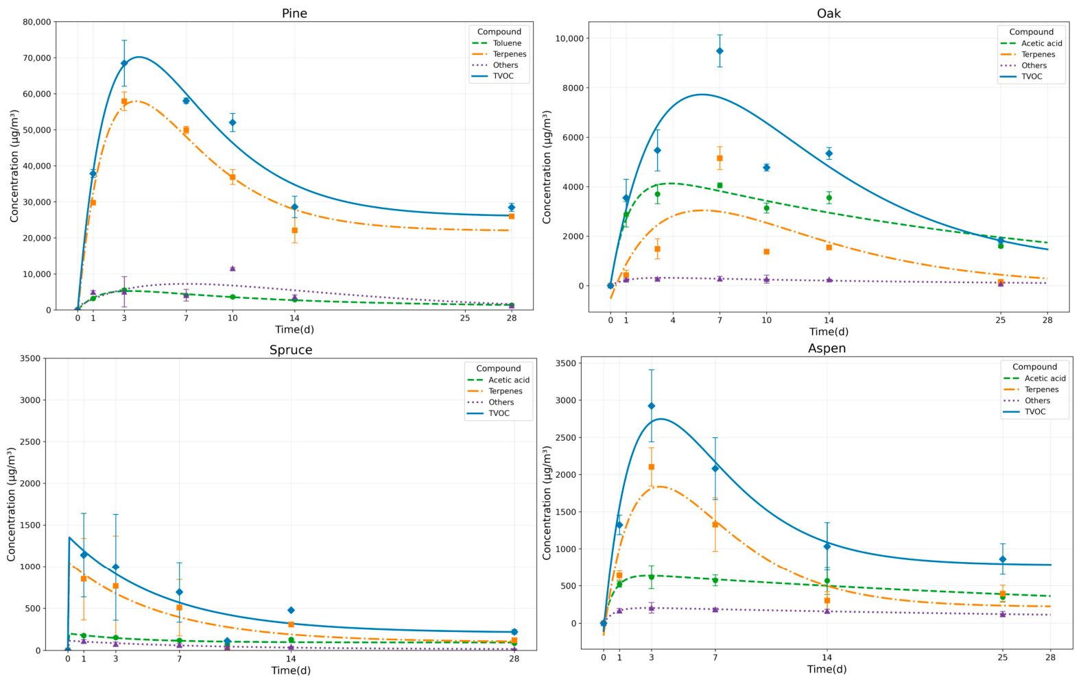
Figure 3 illustrates the primary VOCs emitted from wood samples over 28 days, which together accounted for more than 75% of the TVOC. Table 2 shows the AUC28 results, compared with allowable AUC and H-index. Pine had by far the highest total AUC, followed by oak, whereas aspen and spruce showed substantially lower cumulative emissions. In pine, the emission profile was strongly dominated by C10H16, tentatively identified (TI) as monoterpenes, which accounted for approximately 82% of the total AUC28. The C7H8-related aromatic signal, tentatively assigned to toluene, was the second-largest contributor, representing about 7% of the total AUC28. Although 93 m/z is commonly used as a PTR-MS marker for protonated toluene, the literature indicates that monoterpene-related fragmentation may also contribute to this signal under some conditions [39,54]. This is particularly relevant for pine, whose VOC profile is dominated by terpene-rich resin and extractive compounds. However, the signal is discussed here as a C7H8-related aromatic compound tentatively assigned to toluene to evaluate the worst-case scenario.
Together, these two compounds contributed nearly 90% of the cumulative VOC exposure from pine. The dominance of monoterpenes is consistent with the established emission profile of softwoods, particularly pine, where terpene-rich extractives represent a major source of indoor VOC emissions [15,17].
The H-index for monoterpenes was 1.2, indicating that the cumulative terpene exposure exceeded the allowable AUC over the 28-day period. In contrast, toluene showed a much lower H-index of 0.1. In aspen, the total AUC28 was much lower than in pine. Monoterpenes were still the dominant compound group, contributing approximately 53% of the total AUC, followed by C2H4O2 (TI: Acetic acid), which accounted for about 35%. This is consistent with Adamová, Hradecký and Pánek [17], who reported that low-density hardwoods such as aspen can exhibit softwood-like VOC profiles, attributed to lower lignin density and terpenoid extractives. Although these two compounds together explained most of the cumulative VOC exposure from aspen, their H-index values were low, 0.03 for monoterpenes and 0.10 for acetic acid.
In spruce, the total AUC28 was the lowest among the studied wood species. Monoterpenes contributed around 66% of the total AUC28, while C2H4O2 (TI: Acetic acid) accounted for approximately 24%. It agrees with Hyttinen, Masalin-Weijo, Kalliokoski and Pasanen [49] who reported α-pinene, limonene, and β-pinene as the main emissions from untreated spruce. Despite the relatively high percentage contribution of monoterpenes to spruce emissions, the absolute AUC was low. This was reflected in the H-index values, which were approximately 0.01 for both monoterpenes and acetic acid.
In oak, the cumulative VOC exposure was lower than in pine but higher than aspen and spruce. The emission profile differed from the softwoods, as C2H4O2 (TI: acetic acid) were the dominant contributor, representing approximately 65% of the total AUC28. Monoterpenes contributed about 35%. Oak’s acetic acid-dominated profile agrees with earlier studies identifying oak and other hardwoods as important sources of acetic acid and related oxygenated emissions [48,53]. Gonçalves et al. [55] reported that the precedence and persistence of oak acetic acid is related to hardwood hemicellulose acetyl content for sustained acetic-acid release. The H-index for acetic acid was 0.55, which was below the exceedance threshold. The H-index for monoterpenes was 0.06, indicating a low health-based contribution.
Overall, the H-index showed that the cumulative 28-day exposure remained well below the health-based threshold for all samples and target compounds, except for monoterpenes emitted from pine. This suggests that adverse irritation-related responses are unlikely for aspen, spruce, and oak under the tested conditions. However, for pine, where the H-index for monoterpenes exceeded 1, source-control strategies such as careful material selection, reduced material loading, or enhanced ventilation may be prudent, particularly when pine is used extensively in indoor environments.
The comparison between measured concentrations and LCI values showed that most compounds remained below their health-based reference levels at both baseline and maximum concentrations, except for pine terpenes, pine toluene, oak terpenes, and oak acetates during their peak emission phase (Table 3). Because PTR-MS does not resolve terpene isomers, α-pinene/limonene LCIs were used as conservative surrogates. This approach should be interpreted cautiously, because PTR-MS provides high time resolution but limited structural specificity without chromatographic separation, particularly for isomers and fragment ions [56,57].
In pine, monoterpenes showed the highest exceedance among all samples. The baseline concentration was already well above the LCI value, while the maximum concentration reached approximately 22.8 times the LCI value at 3.7 days. Toluene also exceeded the LCI value at its maximum concentration. However, the baseline concentration was below the LCI value, and the fitted curve indicated that toluene decreased below the threshold after approximately 12–13 days. In oak, both main compounds showed peak concentrations above their LCI values, although their baseline concentrations were negligible. Monoterpenes reached a maximum concentration of approximately 3041 µg/m3 at 3.1 days. The fitted curve indicated that terpene concentrations decreased below the LCI threshold after approximately 10–11 days. Acetates showed a stronger exceedance, reaching a maximum concentration of approximately 4130 µg/m3 at 3.8 days, corresponding to 3.4 times the LCI value. However, acetate concentrations were predicted to fall below the LCI threshold after approximately 37–38 days.

3.2. VVOC Concentration Behaviour Across Wood Samples

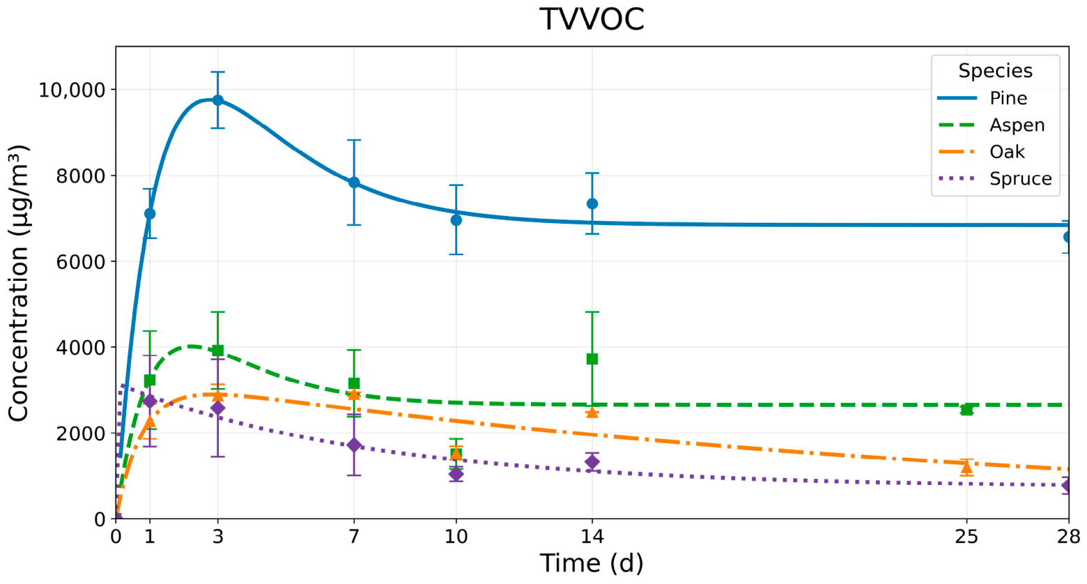
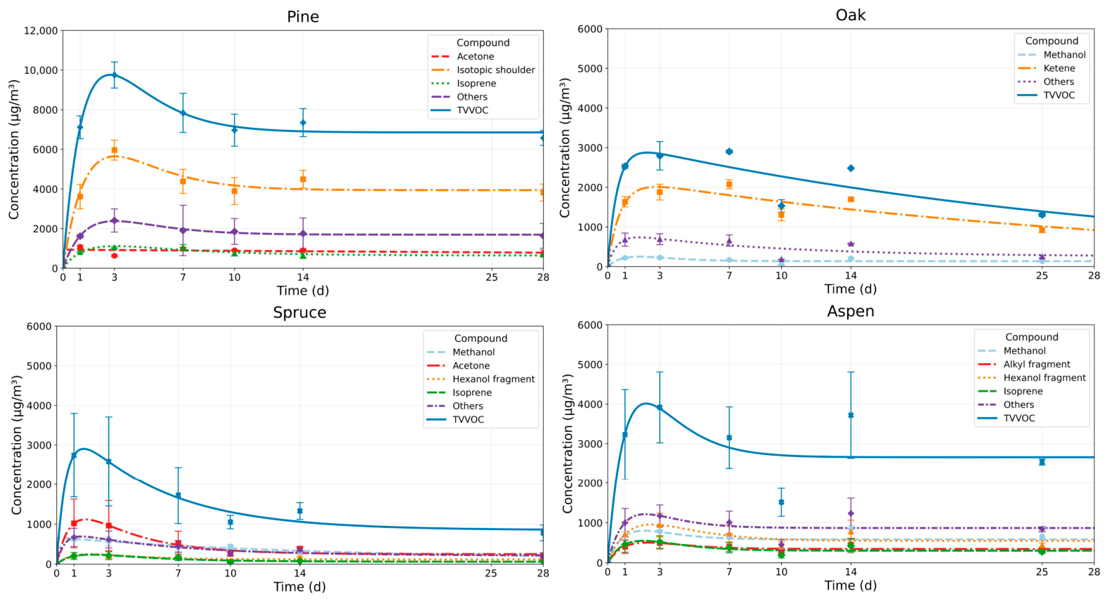
Figure 4 presents the total VVOC accumulated concentration measured from the examined wood samples, and Table 1 summarises the corresponding fitted parameters. Among the investigated species, pine showed the highest VVOC concentration. The concentration reached a maximum of 9756 ± 681 µg/m3 after approximately 2.8 days. This was followed by a rapid decay, characterised by a decay constant of 0.5 ± 0.01 d−1 and a half-time of 1.5 ± 0.09 days. By the end of the experiment, pine stabilised at 6850 ± 451 µg/m3 (Table 1). Aspen showed the second-highest stabilised VVOC concentration among the samples. The maximum concentration reached 4012 ± 1127 µg/m3 after approximately 2.2 days. The decay was relatively rapid, with a decay constant of 0.7 ± 0.02 d−1 and a half-time of 1.1 ± 0.01 days. By day 28, the concentration stabilised at 2657 ± 548 µg/m3. These rapid peak and decay patterns are consistent with the higher volatility and lower retention tendency expected for VVOCs compared with less volatile compounds [58].
Spruce showed lower VVOC concentration than pine and aspen. Its maximum concentration occurred within the first day, reaching 3156 ± 1369 µg/m3. After this early peak, spruce showed a slower decline, with a decay constant of 0.1 ± 0.01 d−1 and a half-time of 5.2 ± 0.01 days. By the end of the experiment, the concentration stabilised at 731 ± 92 µg/m3. The relatively persistent VVOC signal from spruce may indicate that the release of low-molecular oxygenated compounds was not controlled only by volatility, but also by species-specific transport and compound formation processes. Previous studies have reported oxygenated emissions such as methanol and acetone from spruce and other coniferous species, supporting the interpretation that spruce VVOCs may include a substantial oxygenated fraction rather than only rapidly depleted surface compounds [59,60]. Oak showed a distinct VVOC emission profile compared with the other species. The maximum concentration reached 2895 ± 214 µg/m3 after approximately 2.9 ± 1 days. However, the estimated stabilised concentration was 0.0 µg/m3, indicating that the fitted long-term baseline approached zero within the model structure. Oak also showed the longest half-time, 18.4 ± 3 days, suggesting a more gradual decline after the peak. This profile should be interpreted cautiously, because oak VVOCs were dominated by a limited number of tentative ions, and PTR-MS signals at low mass-to-charge ratios may include fragment contributions from oxygenated compounds [57,61].
Overall, the VVOC results indicate that pine was the dominant source, with both the highest peak concentration and the highest stabilised concentration. Aspen also showed a relatively high VVOC emission level, whereas spruce was characterised by an early peak followed by a lower stabilised concentration. Oak differed from the other species by showing a moderate peak but a much longer half-time and a fitted baseline close to zero. From a practical perspective, these results show that VVOCs should not be ignored simply because they are more volatile. Although VVOCs often reached their maximum earlier than VOCs, their persistence and relative contribution differed between wood species. Therefore, the fitted parameters should be interpreted as comparative indicators of early release, relative persistence, and species-specific VVOC behaviour under controlled worst-case conditions, rather than as direct predictions of real indoor concentrations or exact ventilation durations. This supports the need to consider both VOCs and VVOCs when comparing wood materials for indoor use, especially because conventional chamber evaluations and LCI schemes often focus more strongly on VOCs than on VVOCs [58].
Figure 5 illustrates the dominant VVOCs emitted from the wood samples over the 28-day period. In pine, the total VVOC AUC28 was 203.7 ± 18 mg × d/m3. The cumulative profile was dominated by C6H8 (TI: isotopic shoulder of monoterpene), which accounted for 57.8% of the total VVOC AUC28. C3H8 (TI: acetone) and C5H8 (TI: isoprene) were the next major contributors, representing 11.8% and 10.5%, respectively. Together, these three compounds explained approximately 80% of the cumulative VVOC exposure from pine. For compounds with available health-based reference values, the H-index remained below 1. This indicates that, although pine had the highest cumulative VVOC burden, the evaluated compounds did not exceed their allowable AUC thresholds over 28 days (Table 2).
In aspen, the total VVOC AUC28 was 79.2 ± 17 mg × d/m3. The cumulative emissions were more evenly distributed among several compounds than in pine. C6H10 (TI: hexanol fragment) and CH4O (TI: methanol) were the largest contributors, accounting for 21.8% and 21.4% of the total VVOC AUC28, respectively. C5H4 (TI: alkyl fragment) contributed 12.9%, while C5H8 (TI: isoprene) accounted for 11.9%. Together, these four compounds represented approximately 68% of the total cumulative VVOC exposure. The relatively high methanol contribution is chemically plausible, because methanol can originate from cell-wall-related demethylation processes and has been widely discussed as a plant- and wood-related oxygenated volatile [62]. The H-index values for compounds with available reference values were low, indicating that the cumulative exposure remained below the health-based threshold.
In spruce, the total VVOC AUC28 was 37.6 ± 11 mg × d/m3, which was the lowest among the investigated species. C3H8 (TI: acetone) was the dominant contributor, accounting for 30.6% of the total AUC28, followed by CH4O (TI: methanol) at 27.2%. C6H10 (TI: hexanol fragment) and C5H8 (TI: isoprene) contributed 10.4% and 7.4%, respectively. Similarly, Sassoli et al. [63] reported methanol and acetone as oxygenated VOCs emitted by softwoods such as spruce. In the present study, acetone and methanol were the main contributors to the spruce VVOC profile; however, their absolute AUC28 values remained low. Although acetone and methanol were the main contributors to the spruce VVOC profile, their absolute AUC28 values were low. This was reflected in very low H-index values of 0.003 for acetone and 0.005 for methanol. Isoprene also remained below the allowable AUC, with an H-index of 0.07. Therefore, spruce showed the lowest cumulative VVOC exposure and no indication of health-based exceedance for the evaluated compounds.
In oak, the total VVOC AUC28 was 56.0 ± 2 mg × d/m3. Unlike the other species, the cumulative VVOC profile was strongly dominated by C2H2O (TI: ketenes), which accounted for 71.4% of the total VVOC AUC28. CH4O (TI: methanol) was the second identified contributor, but its contribution was much lower, representing only 7.5%. If the C2H2O signal is interpreted as ketene and the corresponding reference value is applied, the H-index indicates a potential exceedance. However, this result should be considered a screening-level concern rather than a definitive toxicological conclusion, because the ion assignment is tentative and PTR-MS signals at this mass may be affected by fragmentation or unresolved oxygenated compounds. This is particularly relevant for oak, where acetic acid-related emissions are expected and acetic acid can produce fragment ions that may interfere with low-mass PTR-MS signals [57,61]. The H-index highlights a primary concern when considering a worst-case scenario: C2H2O (TI: ketenes) from oak (H = 7). This level indicates a significant potential for eye and upper-airway irritation with continuous indoor exposure. Although the C2H2O-related ion is only tentatively assigned to ketene, even a fractional contribution would warrant attention to possible chronic exposure (Table 2).
For VVOCs, the comparison with LCI values was limited because reference values were not available for several of the dominant detected ions (Table 3). In pine, the dominant VVOC signal was C6H8 (TI: isotopic shoulder of monoterpene), with a baseline concentration of 3935.9 ± 519 µg/m3 and a maximum concentration of 5640.9 ± 645 µg/m3 at 3.1 days. C5H8 (TI: isoprene) also peaked at 3.1 days, increasing from 639.2 ± 10 µg/m3 to 1116.8 ± 63 µg/m3. C3H8 (TI: acetone) reached its maximum concentration earlier, within the first day, with a peak value of 934.2 ± 25 µg/m3. Despite this early peak, acetone remained far below its LCI value of 120,000 µg/m3.
In aspen, the main VVOC reached their maximum concentrations between 2.0 and 2.6 days. The highest peak was observed for C6H10 (TI: hexanol fragment), which increased from 546.6 ± 108 µg/m3 to 955.2 ± 301 µg/m3 at 2.6 days. CH4O (TI: methanol) reached a maximum of 800.9 ± 79 µg/m3 at 2.1 days, while C5H8 (TI: isoprene) and C5H4 (TI: alkyl fragment) peaked at 547.6 ± 197 µg/m3 and 503.7 ± 174 µg/m3, respectively.
In spruce, C3H8 (TI: acetone) showed the highest maximum VVOC concentration, increasing from 249.5 ± 3 µg/m3 to 1115.1 ± 693 µg/m3 at 1.7 days. However, this concentration was far below the acetone LCI value of 120,000 µg/m3. CH4O (TI: methanol) reached a maximum of 661.0 ± 59 µg/m3 within the first day. C5H8 (TI: isoprene) and C6H10 (TI: hexanol fragment) showed lower peak concentrations of 236.4 ± 111 µg/m3 and 248.9 ± 88 µg/m3, respectively, at around 2 days. Overall, spruce showed no LCI exceedance for the VVOC with an available reference value. In oak, C2H2O (TI: ketenes) was the dominant VVOC, with a negligible baseline concentration but a maximum concentration of 2008.2 ± 61 µg/m3 at 2.8 days. CH4O (TI: methanol) showed a much lower concentration, increasing from 134.9 ± 14 µg/m3 to 249.0 ± 21 µg/m3 at 1.8 days.
Overall, the VVOC results in Table 3 show that the main compounds generally peaked within the first 1–3 days, with pine showing the highest maximum concentration due to the C6H8 (TI: isotopic shoulder of monoterpene) and oak showing a distinct C2H2O (TI: ketenes)-dominated profile. Among the compounds for which LCI values were available, acetone remained far below the reference level in both pine and spruce. Therefore, no LCI exceedance was observed for the evaluated VVOCs with available health-based reference values. However, the limited availability of VVOC reference values means that the health-based interpretation of VVOCs remains less complete than for VOCs, which is a recognised limitation in current indoor air quality assessment frameworks [58].

3.3. Comparison of VOC vs. VVOC Emissions in Each Sample

Comparing the time behaviour of VVOCs and VOCs showed that VVOCs tended to reach their maximum earlier than VOCs, while the dominant exposure fraction depended strongly on wood species. This is consistent with emission theory, where more volatile compounds are expected to transfer more rapidly from the material surface to the air, while less volatile or more strongly retained compounds may show slower diffusion-controlled release and longer emission tails [64,65].
For pine, VOC concentrations were clearly higher than VVOC concentrations in both peak concentration and cumulative exposure. The VOC peak was approximately seven times higher than the VVOC peak. The same pattern was observed for cumulative exposure, where the VOC AUC28 was 1119.7 ± 58 mg × d/m3 compared with 203.7 ± 18 mg × d/m3 for VVOCs. However, VVOCs decayed faster, with a higher decay constant of 0.5 d−1 and a shorter half-time of 1.5 days. This suggests that pine released the more volatile fraction earlier and more rapidly, whereas VOCs, mainly terpenes, dominated the longer-term emission burden. This behaviour is consistent with the known role of pine extractives as a sustained monoterpene reservoir [16,49].
Aspen showed the opposite pattern in terms of magnitude. The VVOC peak concentration, 4012 ± 1127 µg/m3, was higher than the VOC peak concentration, 2747 ± 450 µg/m3. The cumulative VVOC exposure was also approximately twice the VOC exposure, with AUC28 values of 79.2 ± 17 mg × d/m3 and 38.4 ± 8.6 mg × d/m3, respectively. VVOCs also decayed faster, with a decay constant of 0.7 d−1 and a half-time of 1.1 days, compared with 0.3 d−1 and 2.2 days for VOCs. This indicates that aspen emissions were more influenced by the highly volatile fraction, with faster release and faster decay than the VOC fraction.
Spruce showed an early peak for both VOCs and VVOCs, with maximum concentrations occurring within the first day. However, VVOC emissions were higher than VOC emissions. The VVOC peak was 3156 ± 1369 µg/m3, compared with 1360 ± 625 µg/m3 for VOCs, and the VVOC AUC28 was approximately three times higher than the VOC AUC28. In contrast to pine and aspen, VVOCs decayed more slowly than VOCs in spruce, with a lower decay constant of 0.1 d−1 and a longer half-time of 5.2 days, compared with 0.15 d−1 and 4.1 days for VOCs. This suggests that spruce had a relatively persistent VVOC contribution despite its low total VOC emission level. The result indicates that spruce should not be interpreted only as a low-emitting wood species; rather, its emission profile was low in VOC intensity but relatively enriched in oxygenated VVOCs.
Oak showed a distinct pattern. The VOC peak was higher and occurred later, reaching 7700 ± 730 µg/m3 after 5.8 days, while the VVOC peak reached 2895 ± 214 µg/m3 after 2.9 days. The VOC AUC28 was also higher than the VVOC AUC28, 124 ± 8.4 mg × d/m3 compared with 56.0 ± 2 mg × d/m3. However, the VVOC half-time was much longer, 18.4 days, compared with 3.9 days for VOCs. This indicates a slower decline of the VVOC signal after its early peak. The fitted stabilised VVOC concentration approached zero, while VOCs stabilised at 781 ± 426 µg/m3. This suggests that oak VOC emissions were more persistent in absolute concentration, whereas the VVOC profile was characterised by an early peak followed by a long but declining tail. The delayed oak VOC peak and acetate dominance are consistent with hardwood acetic acid release from acetylated hemicelluloses, which may continue over longer time scales than rapidly depleted surface emissions [48,53].
The general pattern was that VVOCs usually peaked earlier than VOCs, particularly for pine, aspen, and oak. In pine and aspen, VVOCs also showed higher decay constants and shorter half-times, supporting the interpretation of a rapid release phase. However, spruce and oak did not fully follow this pattern, as their VVOC half-times were longer than their VOC half-times. This indicates that VVOC behaviour was not controlled only by volatility, but also by species-specific material structure, compound origin, and delayed release from internal pathways. Overall, VOCs dominated the cumulative exposure in pine and oak, mainly due to high terpene and acetate contributions, whereas VVOCs contributed more strongly than VOCs in aspen and spruce. This shows that total emission behaviour cannot be explained only by volatility class. Instead, both the chemical composition of emissions and the wood species controlled the timing, intensity, and persistence of VOC and VVOC release.
Accordingly, ventilation priorities differed by species. For pine, which exhibited by far the highest peak concentrations and persistently elevated background levels, sustained moderate ventilation combined with source-control measures, such as pre-conditioning or selective sourcing of low-emitting batches, would be required to manage the long-lived TVOC and TVVOC backgrounds. For aspen, emission dynamics were similar in shape to pine but much lower in magnitude, suggesting that sustained moderate ventilation may be sufficient under the tested conditions. For spruce, early high-rate ventilation is likely most effective for reducing the sharp initial peak, followed by steady background ventilation for tail management. For oak, the delayed VOC peak and long VVOC half-time suggest that short-term ventilation alone may be insufficient; longer conditioning and continuous ventilation may be necessary, particularly when oak is used at high material loading.

4. Limitations

This study’s findings should be interpreted with caution due to several limitations.
The passive test chamber method represented a sealed or quasi-static low-ventilation environment under controlled conditions and therefore does not fully reflect real-world emission scenarios for installed wood products. Consequently, reported VOC and VVOC concentrations may be higher than those obtained under standardised dynamic emission chamber conditions or real indoor environments. The model-derived threshold-crossing times should also not be interpreted as real-world clearance times or as practical predictions of how long installed wood products require to reach acceptable concentrations. Instead, these values should be used only as comparative indicators of relative persistence among wood species and compound groups under the specific experimental conditions applied in this study.
In addition, periodic PTR-TOF-MS sampling introduced a small effective air exchange, estimated as 0.24 ± 0.06 air changes per measurement and approximately 1.4 ± 0.4 air changes over the full experiment. Therefore, the observed post-peak decline reflects both material emission behaviour and minor sampling-induced dilution. Emissions were also measured only from kiln-dried, untreated boards of four wood species under controlled temperature and relative humidity conditions. The results may therefore not be directly transferable to other wood products, surface treatments, material ages, higher temperatures, different humidity levels, or longer-term indoor scenarios.
The PTR-TOF-MS method offers high sensitivity and real-time detection, which was useful for following the time-resolved development of VOC and VVOC headspace profiles. However, the method also has important constraints. Because only acetone was used as an external calibration standard, compound-specific response factors were not available for most detected ions. Therefore, the reported concentrations should be considered semi-quantitative for compounds without authentic calibration standards. The results are most robust for comparing relative temporal behaviour and differences between wood species measured under the same experimental conditions.
PTR-TOF-MS quantification may also be affected by humidity, compound-dependent ionisation efficiency, fragmentation behaviour, and changes in headspace composition during closed-chamber accumulation. Although temperature and relative humidity were controlled, the chemical composition of the sealed headspace changed over time as VOCs and VVOCs accumulated. This may have influenced proton-transfer reaction rates, ionisation efficiency, and the relative abundance of parent and fragment ions. These effects should be considered when interpreting absolute concentrations and compound-specific comparisons.
Compound identification in PTR-TOF-MS is based mainly on accurate mass and library-supported tentative assignment. Therefore, structural isomers and in-source fragments can share identical or overlapping m/z values, and assignments should be regarded as tentative unless confirmed by chromatographic separation or reference standards. This limitation is particularly relevant for isomeric or fragment-prone signals, including C7H8-related aromatic compounds and low-mass oxygenated ions. Accordingly, PTR-TOF-MS was used in this study primarily as a comparative, time-resolved screening tool rather than as a definitive compound-identification or absolute-quantification method.
The ion at m/z 31, tentatively related to formaldehyde, is particularly sensitive to interferences and humidity effects; chromatographic pre-separation is required for reliable compound-specific analysis. Because such corrections were beyond the scope of the present study, m/z 31 was treated as an unresolved oxygenated signal and was excluded from compound-specific kinetics and health-risk metrics, in line with community guidance. Several ions with ambiguous elemental formulas, such as m/z 42.030 and 71.09, were likewise classified as unresolved and retained only for bulk-TVOC/TVVOC decay modelling to preserve mass balance and stable kinetic fits. Inclusion of unresolved ions can inflate bulk totals, particularly at early times; therefore, health-impact assessments were restricted to tentatively identified compounds with available reference values.
The limited availability of health-based reference values for VVOCs also restricted the benchmarking capability of this study. As a result, the health-based interpretation is more complete for VOCs than for several VVOC signals. For future studies, chromatographic pre-separation should be integrated with PTR-MS, for example, through GC-MS/MS, headspace GC-MS/MS, or GC-PTR-MS, to confirm uncertain assignments, separate structural isomers, and improve compound-specific quantification. Future work should also extend monitoring under dynamic chamber conditions and realistic indoor scenarios, including representative ventilation rates, material loading, air mixing, temperature, humidity, surface-sink effects, and a broader range of low-emission surface treatments, particularly water-based or bio-based treatments.

5. Conclusions

This study provides a comparative, time-resolved screening of VOC and VVOC accumulation from four untreated wood species under controlled quasi-static, low-ventilation conditions. The results help to identify species- and compound-dependent differences in peak timing, concentration magnitude, post-peak decline, and relative persistence under the same controlled worst-case conditions.
Pine showed the highest VOC burden among the investigated species, with the highest peak concentration, highest late-stage concentration, and highest AUC28. Its accumulated VOC profile was dominated by monoterpenes, indicating that pine can act as a strong and persistent source of terpene-related VOCs under low-ventilation conditions. The C7H8-related aromatic signal in pine, tentatively assigned to toluene, exceeded the toluene reference value during the peak phase in a screening-level comparison. Because this signal was not chromatographically confirmed, it should not be interpreted as definitive evidence of toluene emission from pine. These findings indicate that pine should be managed primarily through source-control measures, including careful material selection, reduced exposed loading, and pre-conditioning before installation, with sustained ventilation used as a complementary measure rather than as the sole mitigation strategy.
Oak showed a distinct temporal profile compared with the other species. Although its total VOC burden was lower than pine, it showed the second-highest VOC AUC28 and a delayed oxygenated emission profile, mainly associated with C2H4O2-related compounds tentatively assigned to acetic acid. This delayed decline suggests that oak may require longer conditioning and sustained ventilation than species with faster emission decay. Furthermore, it should be considered that the short-term testing alone may underestimate the contribution of some wood species, particularly when relevant compounds peak later than the first measurement period. Aspen and spruce showed lower VOC burdens under the tested conditions, but their VVOC contributions were relatively important, showing that lower-emitting wood species should not be assessed only using conventional TVOC metrics.
Across species, VVOCs generally peaked earlier than VOCs in pine, aspen, and oak, supporting the interpretation that the more volatile fraction is released more rapidly during the initial emission phase. Spruce was the exception, with both VOCs and VVOCs peaking within the first day. However, the longer VVOC half-times observed for spruce and oak indicate that VVOC behaviour was not controlled by volatility alone, but also by wood chemistry, compound origin, and internal transport processes.
Overall, the findings show that emission behaviour cannot be explained by volatility class alone. Wood species, chemical composition, material structure, and compound-specific health thresholds jointly controlled the timing, intensity, persistence, and relevance of emissions. The observed post-peak decline should therefore be understood as part of the chamber source–sink behaviour, involving depletion of readily available compound reservoirs, sorption to chamber surfaces, re-partitioning between the wood and headspace, and minor sampling-induced dilution. The practical message of this work is that wood materials should be compared not only by total VOC concentration, but also by the timing and persistence of their dominant VOC and VVOC fractions. Pine requires particular attention because of its high and persistent terpene-related burden, oak because of its delayed oxygenated profile, and aspen and spruce because their lower VOC profiles may still include relevant VVOC contributions. Translation of these findings into real-world building guidance requires further validation under dynamic chamber or realistic indoor conditions, including representative ventilation rates, material loading, air mixing, temperature, humidity, and indoor surface-sink effects.

Author Contributions

Conceptualization, S.G.J. and H.K.N.; methodology, S.G.J., J.F.D. and S.R.S.; software, S.G.J. and S.O.N.; validation, S.G.J., S.O.N., H.K.N. and T.S.V.; formal analysis, S.G.J. and S.O.N. resources, H.K.N. and S.G.J.; data curation, S.G.J. and S.O.N.; writing—original draft preparation, S.G.J.; writing—review and editing, H.K.N. and T.S.V.; visualization, S.G.J.; supervision, H.K.N. and T.S.V.; project administration, S.G.J., H.K.N. and T.S.V.; funding acquisition, S.G.J., H.K.N. and T.S.V. All authors have read and agreed to the published version of the manuscript.

Funding

This work was supported by the framework of the K-HEALTHinAIR project funded by the European Union under Grant agreement ID: 101057693. The views and opinions expressed are those of the authors only and do not necessarily reflect those of the European Union or HADEA.

Institutional Review Board Statement

This research involved only non-living material samples and did not include human participants, animals, or personal data. Consent to participate and consent for publication are not applicable.

Data Availability Statement

The datasets analysed for this study can be found in Zenodo [40]. Time-resolved VOC and VVOC accumulation data from untreated wood species under quasi-static low-ventilation conditions, [Data set]. Zenodo. https://doi.org/10.5281/zenodo.21444573.

Acknowledgments

The authors would like to acknowledge the valuable support provided by CARTIF Technology Centre for granting access to its library and PTR-MS instrumentation, as well as for assistance with raw data analysis using IDA and the calibration process. The authors also thank Alberto Moral Quiza, Head of CARTIF Technology Centre, for his support of the project, and Alicia Aguado Pesquera for her assistance with methodology development and laboratory resources. The authors further acknowledge Bergene Holm AS for providing the wood samples used in this study. During the preparation of this manuscript, the authors used ChatGPT 5 (OpenAI) to assist with language polishing, improving readability, and minor reorganisation of the text. All AI-generated content was carefully reviewed and edited by the authors, who take full responsibility for the final content of the manuscript. No AI tools were used for data collection, statistical analysis, interpretation of the results, or drawing scientific conclusions, and no confidential or proprietary information was entered into the tool.

Conflicts of Interest

This research was conducted in collaboration with CARTIF Technology Center as part of the K-HEALTHinAIR project. The funder and collaborating institution had no role in the study design, data collection and analysis, decision to publish, or preparation of the manuscript. The authors declare that the research was conducted in the absence of any commercial or financial relationships that could be construed as a potential conflict of interest. The authors report there are no competing interests to declare.

Abbreviations

The following abbreviations and symbols are used in this manuscript:
ACGIHAmerican Conference of Governmental Industrial Hygienists
ACTRISAerosol, Clouds and Trace Gases Research Infrastructure
AUCArea under the concentration–time curve
AUC28Area under the concentration–time curve over 28 days
CVCoefficient of variation
DaDalton
E/NRatio of electric field strength to drift-gas number density
ENEuropean Standard
GC-MSGas Chromatography–Mass Spectrometry
GC-PTR-MSGas Chromatography–Proton Transfer Reaction Mass Spectrometry
GLOVOCSMaster compound assignment guide for PTR-MS users
H-indexHazard index
IAQIndoor air quality
IFEmpirical yield factor
ISOInternational Organization for Standardization
LCILowest Concentration of Interest
LCULiquid Calibration Unit
m/zMass-to-charge ratio
PTR-MSProton Transfer Reaction Mass Spectrometry
PTR-TOF-MSProton Transfer Reaction–Time-of-Flight Mass Spectrometry
QA/QCQuality assurance/quality control
RHRelative humidity
RRIDResearch Resource Identifier
TITentative identification
TLVThreshold Limit Value
TLV-TWAThreshold Limit Value–Time-Weighted Average
TVOCTotal volatile organic compounds
TVVOCTotal very volatile organic compounds
UiAUniversity of Agder
VOC(s)Volatile organic compound(s)
VVOC(s)Very volatile organic compound(s)

References

  1. Bastien, D.; Winther-Gaasvig, M.; Zhang Andersson, J.; Xiao, Z.; Ge, H. Hygrothermal Performance of Natural Building Materials: Simulations and Field Monitoring of a Case Study Home Made of Wood Fiber Insulation and Clay. J. Build. Phys. 2023, 47, 249–283. [Google Scholar] [CrossRef]
  2. Lee, J.-H.; Kim, J.; Kim, S.; Kim, J.T. Thermal Extractor Analysis of VOCs Emitted from Building Materials and Evaluation of the Reduction Performance of Exfoliated Graphite Nanoplatelets. Indoor Built Environ. 2013, 22, 68–76. [Google Scholar]
  3. Shao, H.; Guo, Z.; Li, W.; Fang, L.; Qin, M.; Cai, H.; Zhang, Y.; Guan, B.; Wu, C.; Liu, J. Three-Dimensional Geometry, Pore Parameter, and Fractal Characteristic Analyses of Medium-Density Fiberboard by X-Ray Tomography, Coupling with Scanning Electron Microscopy and Mercury Intrusion Porosimetry. J. Build. Phys. 2021, 44, 364–382. [Google Scholar]
  4. Lee, C.-S.; Haghighat, F.; Ghaly, W. Conjugate Mass Transfer Modeling for VOC Source and Sink Behavior of Porous Building Materials: When to Apply It? J. Build. Phys. 2006, 30, 91–111. [Google Scholar] [CrossRef]
  5. United States Environmental Protection Agency. Indoor Air Quality (IAQ). Available online: https://www.epa.gov/indoor-air-quality-iaq (accessed on 12 April 2026).
  6. Tsai, W.-T. An Overview of Health Hazards of Volatile Organic Compounds Regulated as Indoor Air Pollutants. Rev. Environ. Health 2019, 34, 81–89. [Google Scholar] [PubMed]
  7. Rumchev, K.; Spickett, J.; Bulsara, M.; Phillips, M.; Stick, S. Association of Domestic Exposure to Volatile Organic Compounds with Asthma in Young Children. Thorax 2004, 59, 746–751. [Google Scholar] [CrossRef] [PubMed]
  8. Kotzias, D. Built Environment and Indoor Air Quality: The Case of Volatile Organic Compounds. AIMS Environ. Sci. 2021, 8, 135–147. [Google Scholar] [CrossRef]
  9. Pye, H.; Appel, K.; Seltzer, K.; Ward-Caviness, C.; Murphy, B. Human-Health Impacts of Controlling Secondary Air Pollution Precursors. Environ. Sci. Technol. Lett. 2022, 9, 96–101. [Google Scholar] [CrossRef] [PubMed]
  10. Dong, Z.; Jiang, Y.; Wang, S.; Xing, J.; Ding, D.; Zheng, H.; Wang, H.; Huang, C.; Yin, D.; Song, Q.; et al. Spatially and Temporally Differentiated NOx and VOCs Emission Abatement Could Effectively Gain O3-Related Health Benefits. Environ. Sci. Technol. 2024, 58, 19372–19383. [Google Scholar] [CrossRef]
  11. Arata, C.; Misztal, P.; Tian, Y.; Lunderberg, D.; Kristensen, K.; Novoselac, A.; Vance, M.; Farmer, D.; Nazaroff, W.; Goldstein, A. Volatile Organic Compound Emissions during HOMEChem. Indoor Air 2021, 31, 2099–2117. [Google Scholar] [CrossRef] [PubMed]
  12. Davis, A.Y.; Zhang, Q.; Wong, J.P.S.; Weber, R.J.; Black, M.S. Characterization of Volatile Organic Compound Emissions from Consumer Level Material Extrusion 3D Printers. Build. Environ. 2019, 160, 106209. [Google Scholar] [CrossRef]
  13. Sollinger, S.; Levsen, K.; Wünsch, G. Indoor Pollution by Organic Emissions from Textile Floor Coverings: Climate Test Chamber Studies under Static Conditions. Atmos. Environ. 1994, 28, 2369–2378. [Google Scholar] [CrossRef]
  14. Fujitani, Y.; Sato, K.; Tanabe, K.; Morino, Y.; Takahashi, K.; Hoshi, J. Characteristics of Different Volatility Classes of Organic Compounds Emitted by a Municipal Solid Waste Incineration Plant. Atmos. Environ. X 2023, 20, 100225. [Google Scholar]
  15. Pohleven, J.; Burnard, M.D.; Kutnar, A. Volatile Organic Compounds Emitted from Untreated and Thermally Modified Wood—A Review. Wood Fiber Sci. 2019, 51, 231–254. [Google Scholar] [CrossRef]
  16. Czajka, M.; Fabisiak, B.; Fabisiak, E. Emission of Volatile Organic Compounds from Heartwood and Sapwood of Selected Coniferous Species. Forests 2020, 11, 92. [Google Scholar] [CrossRef]
  17. Adamová, T.; Hradecký, J.; Pánek, M. Volatile Organic Compounds (VOCs) from Wood and Wood-Based Panels: Methods for Evaluation, Potential Health Risks, and Mitigation. Polymers 2020, 12, 2289. [Google Scholar] [CrossRef] [PubMed]
  18. Junge, K.M.; Buchenauer, L.; Elter, E.; Butter, K.; Kohajda, T.; Herberth, G.; Röder, S.; Borte, M.; Kiess, W.; von Bergen, M.; et al. Wood Emissions and Asthma Development: Results from an Experimental Mouse Model and a Prospective Cohort Study. Environ. Int. 2021, 151, 106449. [Google Scholar] [CrossRef] [PubMed]
  19. Alapieti, T.; Castagnoli, E.; Salo, L.; Mikkola, R.; Pasanen, P.; Salonen, H. The Effects of Paints and Moisture Content on the Indoor Air Emissions from Pinewood (Pinus sylvestris) Boards. Indoor Air 2021, 31, 1563–1576. [Google Scholar] [CrossRef] [PubMed]
  20. Wojnowski, W.; Kalinowska, K.; Majchrzak, T.; Zabiegała, B. Real-Time Monitoring of the Emission of Volatile Organic Compounds from Polylactide 3D Printing Filaments. Sci. Total Environ. 2021, 805, 150181. [Google Scholar] [PubMed]
  21. Kwok, N.-H.; Lee, S.-C.; Guo, H.; Hung, W.-T. Substrate Effects on VOC Emissions from an Interior Finishing Varnish. Build. Environ. 2003, 38, 1019–1026. [Google Scholar] [CrossRef]
  22. Ghaffari Jabbari, S.; Fermoso Domínguez, J.; Rodríguez Sufuentes, S.; Nyberg, S.O.; Sandnes Vehus, T.; Kofoed Nielsen, H. VOC Emission from Commercial Wood Panels by Proton Transfer Reaction—Analysis for Indoor Air Quality. Front. Built Environ. 2025, 11, 1545306. [Google Scholar] [CrossRef]
  23. EN 16516; Construction Products: Assessment of Release of Dangerous Substances—Determination of Emissions into Indoor Air. European Committee for Standardization: Brussels, Belgium, 2020.
  24. Cappellin, L.; Biasioli, F.; Granitto, P.M.; Schuhfried, E.; Soukoulis, C.; Costa, F.; Märk, T.D.; Gasperi, F. On Data Analysis in PTR-TOF-MS: From Raw Spectra to Data Mining. Sens. Actuators B Chem. 2011, 155, 183–190. [Google Scholar] [CrossRef]
  25. Jensen, A.R.; Koss, A.R.; Hales, R.B.; de Gouw, J.A. Measurements of Volatile Organic Compounds in Ambient Air by Gas-Chromatography and Real-Time Vocus PTR-TOF-MS: Calibrations, Instrument Background Corrections, and Introducing a PTR Data Toolkit. Atmos. Meas. Tech. 2023, 16, 5261–5285. [Google Scholar] [CrossRef]
  26. Müller, M.; Mikoviny, T.; Jud, W.; D’Anna, B.; Wisthaler, A. A New Software Tool for the Analysis of High Resolution PTR-TOF Mass Spectra. Chemom. Intell. Lab. Syst. 2013, 127, 158–165. [Google Scholar] [CrossRef]
  27. Cappellin, L.; Biasioli, F.; Schuhfried, E.; Soukoulis, C.; Märk, T.D.; Gasperi, F. Extending the dynamic range of proton transfer reaction time-of-flight mass spectrometers by a novel dead time correction. Rapid Commun. Mass Spectrom. 2011, 25, 179. [Google Scholar] [PubMed]
  28. Yáñez-Serrano, A.M.; Filella, I.; Llusià, J.; Gargallo-Garriga, A.; Granda, V.; Bourtsoukidis, E.; Williams, J.; Seco, R.; Cappellin, L.; Werner, C.; et al. GLOVOCS—Master Compound Assignment Guide for Proton Transfer Reaction Mass Spectrometry Users. Atmos. Environ. 2021, 244, 117929. [Google Scholar] [CrossRef]
  29. Taiti, C.; Costa, C.; Menesatti, P.; Comparini, D.; Bazihizina, N.; Azzarello, E.; Masi, E.; Mancuso, S. Class-Modeling Approach to PTR-TOFMS Data: A Peppers Case Study. J. Sci. Food Agric. 2015, 95, 1757–1763. [Google Scholar] [PubMed]
  30. Dusanter, S.; Holzinger, R.; Klein, F.; Salameh, T.; Jamar, M. Measurement Guidelines for VOC Analysis by PTR-MS; IMT Nord Europe, Institut Mines Télécom: Lille, France, 2025. [Google Scholar]
  31. Holzinger, R.; Acton, W.J.F.; Bloss, W.J.; Breitenlechner, M.; Crilley, L.R.; Dusanter, S.; Gonin, M.; Gros, V.; Keutsch, F.N.; Kiendler-Scharr, A.; et al. Validity and Limitations of Simple Reaction Kinetics to Calculate Concentrations of Organic Compounds from Ion Counts in PTR-MS. Atmos. Meas. Tech. 2019, 12, 6193–6208. [Google Scholar] [CrossRef]
  32. Coggon, M.M.; Stockwell, C.E.; Claflin, M.S.; Pfannerstill, E.Y.; Xu, L.; Gilman, J.B.; Marcantonio, J.; Cao, C.; Bates, K.; Gkatzelis, G.I.; et al. Identifying and Correcting Interferences to PTR-TOF-MS Measurements of Isoprene and Other Urban Volatile Organic Compounds. Atmos. Meas. Tech. 2024, 17, 801–825. [Google Scholar] [CrossRef]
  33. De Gouw, J.; Warneke, C. Measurements of Volatile Organic Compounds in the Earth’s Atmosphere Using Proton-Transfer-Reaction Mass Spectrometry. Mass Spectrom. Rev. 2007, 26, 223–257. [Google Scholar] [PubMed]
  34. Ruuskanen, T.M.; Kolari, P.; Bäck, J.; Kulmala, M.; Rinne, J.; Hakola, H.; Taipale, R.; Raivonen, M.; Altimir, N.; Hari, P. On-Line Field Measurements of Monoterpene Emissions from Scots Pine by Proton-Transfer-Reaction Mass Spectrometry. Boreal Environ. Res. 2005, 10, 553–567. [Google Scholar]
  35. Tani, A.; Hayward, S.; Hewitt, C.N. Measurement of Monoterpenes and Related Compounds by Proton Transfer Reaction-Mass Spectrometry (PTR-MS). Int. J. Mass Spectrom. 2003, 223, 561–578. [Google Scholar] [CrossRef]
  36. Warneke, C.; de Gouw, J.A.; Kuster, W.C.; Goldan, P.D.; Fall, R. Validation of Atmospheric VOC Measurements by Proton-Transfer-Reaction Mass Spectrometry Using a Gas-Chromatographic Preseparation Method. Environ. Sci. Technol. 2003, 37, 2494–2501. [Google Scholar] [CrossRef] [PubMed]
  37. Li, F.; Huang, D.D.; Tian, L.; Yuan, B.; Tan, W.; Zhu, L.; Ye, P.; Worsnop, D.; Hoi, K.I.; Mok, K.M.; et al. Response of Protonated, Adduct, and Fragmented Ions in Vocus Proton-Transfer-Reaction Time-of-Flight Mass Spectrometer (PTR-TOF-MS). Atmos. Meas. Tech. 2024, 17, 2415–2427. [Google Scholar] [CrossRef]
  38. ISO 16000-6:2021; Indoor Air—Part 6: Determination of Volatile Organic Compounds in Indoor and Test Chamber Air by Active Sampling on Tenax TA Sorbent, Thermal Desorption and Gas Chromatography Using MSD/FID. ISO: Geneva, Switzerland, 2021.
  39. Ambrose, J.L.; Haase, K.; Russo, R.; Zhou, Y.; White, M.; Frinak, E.; Jordan, C.; Mayne, H.R.; Talbot, R.; Sive, B.C. A comparison of GC-FID and PTR-MS toluene measurements in ambient air under conditions of enhanced monoterpene loading. Atmos. Meas. Tech. 2010, 3, 959–980. [Google Scholar] [CrossRef]
  40. Ghaffari Jabbari, S.; Fermoso Domínguez, J.; Rodríguez Sufuentes, S. Dynamic Emission Profile of VOCs and VVOCs [Data Set]; Zenodo: Geneva, Switzerland, 2026. [Google Scholar]
  41. Python Software Foundation. Python Language Reference, Version 3.11; Python Software Foundation: Beaverton, OR, USA, 2022. Available online: https://www.python.org (accessed on 1 May 2026).
  42. Guo, H.; Murray, F.; Lee, S.-C. Emissions of Total Volatile Organic Compounds from Pressed Wood Products in an Environmental Chamber. Build. Environ. 2002, 37, 1117–1126. [Google Scholar] [CrossRef]
  43. Lee, C.; Yang, W.; Parr, R.G. Development of the Colle-Salvetti Correlation-Energy Formula into a Functional of the Electron Density. Phys. Rev. B 1988, 37, 785–789. [Google Scholar] [CrossRef]
  44. Colombo, A.; De Bortoli, M.; Pecchio, E.; Schauenburg, H.; Schlitt, H.; Vissers, H. Chamber Testing of Organic Emission from Building and Furnishing Materials. Sci. Total Environ. 1990, 91, 237–249. [Google Scholar] [CrossRef] [PubMed]
  45. American Conference of Governmental Industrial Hygienists (ACGIH). TLVs and BEIs: Threshold Limit Values for Chemical Substances and Physical Agents & Biological Exposure Indices; ACGIH: Cincinnati, OH, USA, 2023. [Google Scholar]
  46. Canadian Centre for Occupational Health and Safety. Occupational Hygiene—Occupational Exposure Limits. Available online: https://www.ccohs.ca/oshanswers/hsprograms/occ_hygiene/occ_exposure_limits.html (accessed on 7 August 2025).
  47. Gaylor, D.W. The Use of Haber’s Law in Standard Setting and Risk Assessment. Toxicology 2000, 149, 17–19. [Google Scholar] [CrossRef] [PubMed]
  48. Risholm-Sundman, M.; Lundgren, M.; Vestin, E.; Herder, P. Emissions of Acetic Acid and Other Volatile Organic Compounds from Different Species of Solid Wood. Holz Roh Werkst. 1998, 56, 125–129. [Google Scholar] [CrossRef]
  49. Hyttinen, M.; Masalin-Weijo, M.; Kalliokoski, P.; Pasanen, P. Comparison of VOC Emissions between Air-Dried and Heat-Treated Norway Spruce (Picea abies), Scots Pine (Pinus sylvestris) and European Aspen (Populus tremula) Wood. Atmos. Environ. 2010, 44, 5028–5033. [Google Scholar] [CrossRef]
  50. Lee, C.-S.; Haghighat, F.; Ghaly, W. A study on VOC source and sink behavior in porous building materials–analytical model development and assessment. Indoor Air 2005, 15, 183–196. [Google Scholar] [CrossRef] [PubMed]
  51. Jørgensen, R.B.; Dokka, T.H.; Bjørseth, O. Introduction of a sink-diffusion model to describe the interaction between volatile organic compounds (VOCs) and material surfaces. Indoor Air 2000, 10, 27–38. [Google Scholar] [CrossRef] [PubMed]
  52. Yang, X.; Chen, Q.; Zhang, J.; An, Y.; Zeng, J.; Shaw, C. A mass transfer model for simulating VOC sorption on building materials. Atmos. Environ. 2001, 35, 1291–1299. [Google Scholar] [CrossRef]
  53. Gibson, L.T.; Watt, C.M. Acetic and Formic Acids Emitted from Wood Samples and Their Effect on Selected Materials in Museum Environments. Corros. Sci. 2010, 52, 172–178. [Google Scholar] [CrossRef]
  54. Tani, A. Fragmentation and reaction rate constants of terpenoids determined by proton transfer reaction-mass spectrometry. Environ. Control Biol. 2013, 51, 23–29. [Google Scholar] [CrossRef]
  55. Gonçalves, F.D.; Carvalho, L.H.; Rodrigues, J.A.; Ramos, R.M. Wood-Based Panels and Volatile Organic Compounds (VOCs): An Overview on Production, Emission Sources and Analysis. Molecules 2025, 30, 3195. [Google Scholar] [CrossRef] [PubMed]
  56. Blake, R.; Monks, P.; Ellis, A. Proton-Transfer Reaction Mass Spectrometry. Chem. Rev. 2009, 109, 861–896. [Google Scholar] [CrossRef] [PubMed]
  57. Ditto, J.C.; Huynh, H.N.; Yu, J.; Link, M.F.; Poppendieck, D.; Claflin, M.S.; Vance, M.E.; Farmer, D.K.; Chan, A.W.H.; Abbatt, J.P.D. Speciating Volatile Organic Compounds in Indoor Air: Using in Situ GC to Interpret Real-Time PTR-MS Signals. Environ. Sci. Process. Impacts 2025, 27, 1671–1687. [Google Scholar] [CrossRef]
  58. Salthammer, T. Very Volatile Organic Compounds: An Understudied Class of Indoor Air Pollutants. Indoor Air 2016, 26, 25–38. [Google Scholar] [PubMed]
  59. Janson, R.; de Serves, C. Acetone and Monoterpene Emissions from the Boreal Forest in Northern Europe. Atmos. Environ. 2001, 35, 4629–4637. [Google Scholar] [CrossRef]
  60. Filella, I.; Wilkinson, M.J.; Llusia, J.; Hewitt, C.N.; Peñuelas, J. Volatile Organic Compounds Emissions in Norway Spruce (Picea abies) in Response to Temperature Changes. Physiol. Plant. 2007, 130, 58–66. [Google Scholar] [CrossRef]
  61. Baasandorj, M.; Millet, D.B.; Hu, L.; Mitroo, D.; Williams, B.J. Measuring Acetic and Formic Acid by Proton-Transfer-Reaction Mass Spectrometry: Sensitivity, Humidity Dependence, and Quantifying Interferences. Atmos. Meas. Tech. 2015, 8, 1303–1321. [Google Scholar] [CrossRef]
  62. Dorokhov, Y.L.; Sheshukova, E.V.; Komarova, T.V. Methanol in Plant Life. Front. Plant Sci. 2018, 9, 1623. [Google Scholar] [CrossRef] [PubMed]
  63. Sassoli, M.; Taiti, C.; Guidi Nissim, W.; Costa, C.; Mancuso, S.; Menesatti, P.; Fioravanti, M. Characterization of VOC Emission Profile of Different Wood Species during Moisture Cycles. iForest 2017, 10, 576–584. [Google Scholar] [CrossRef]
  64. Salthammer, T. Acetaldehyde in the Indoor Environment. Environ. Sci. Atmos. 2023, 3, 474–493. [Google Scholar] [CrossRef]
  65. Xiong, J.; Liu, C.; Zhang, Y. A General Analytical Model for Formaldehyde and VOC Emission/Sorption in Single-Layer Building Materials and Its Application in Determining the Characteristic Parameters. Atmos. Environ. 2012, 47, 288–294. [Google Scholar] [CrossRef]
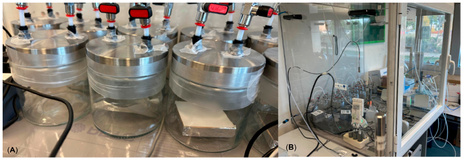
Figure 1. Experimental setup for time-resolved VOC and VVOC headspace measurements from wood samples: (A) glass chamber; (B) climate-controlled chamber.
Forests 17 00884 g001
Figure 2. Time-dependent TVOC emission profiles across wood species.
Forests 17 00884 g002
Figure 3. Bi-exponential model fits of total and fractionated VOC emissions for aspen, oak, pine, and spruce.
Forests 17 00884 g003
Figure 4. Bi-exponential model fits of total and fractionated VVOC emissions for aspen, oak, pine, and spruce.
Forests 17 00884 g004
Figure 5. Dominant VVOCs emitted from the wood samples over the 28-day period.
Forests 17 00884 g005
Table 1. Bi-exponential model parameters describing VOC and VVOC emissions from different wood species.
SpeciesC [µg/m3]Half-Time [d]Peak Time [d]Peak Value [µg/m3]a [d−1]R2
VOCPine25,800 ± 1590 (CV = 6%)2.3 ± 0.023.9 ± 0.0170,100 ± 3500 (CV = 5%)0.3 ± 0.04 (CV = 12%)0.97
Aspen778 ± 215 (CV = 27%)2.2 ± 0.083.6 ± 0.12747 ± 450 (CV = 16%)0.3 ± 0.01 (CV = 3%)0.97
Spruce207 ± 114 (CV = 55%)4.1 ± 1.9<11360 ± 625 (CV = 44%)0.15 ± 0.03 (CV = 20%)0.87
Oak781 ± 426 (CV = 56%)3.9 ± 0.385.8 ± 0.47700 ± 730 (CV = 9.5%)0.17 ± 0.02 (CV = 9%)0.85
VVOCPine6850.1 ± 451 (CV = 7%)1.5 ± 0.092.8 ± 0.019756.1 ± 681 (CV = 7%)0.45 ± 0.01 (CV = 51%)0.99
Aspen2657.2 ± 548 (CV = 21%)1.1 ± 0.012.2 ± 0.014011.5 ± 1127 (CV = 28%)0.65 ± 0.02 (CV = 6%)0.81
Oak0.0 (CV = NA)18.4 ± 32.9 ± 12894.6 ± 214 (CV = 7%)0.03 (CV = 20%)0.91
Spruce731.3 ± 92 (CV = 13%)5.2 ± 0.01<13156.1 ± 1369 (CV = 43%)0.13 ± 0.01 (CV = 5%)0.99
Table 2. Cumulative exposure to main compounds and TVOC for 28 days, and health risk indicators.
Gas TypeWood TypeTotal AUC28 [mg × d/m3]Main
Compounds
AUC28
[mg × d/m3]
% of Total AUC8-h TWA [mg × h/m3]Allowable AUC
[mg × d/m3]
H-Index
VOCsPine1119.7 ± 58
(CV = 5.2%)
Terpenes (C10H16)914.7 ± 39
(CV = 4.3%)
82111.3742.01.2
Toluene (C7H8)81.5 ± 1.7
(CV = 2.1%)
775.3502.00.16
Aspen38.4 ± 8.6
(CV = 22%)
Terpenes (C10H16)20.5 ± 4.9
(CV = 24%)
53111.3662.50.03
Acetic acid (C2H4O2)13.7 ± 3
(CV = 22%)
3524.5145.80.1
Spruce12.7 ± 3.7
(CV = 29%)
Terpenes (C10H16)8.4 ± 3.7
(CV = 43%)
66.2111.3742.00.01
Acetic acid (C2H4O2)3.1 ± 0.1
(CV = 4.3%)
24.324.5163.30.01
Oak124 ± 8.4
(CV = 6.8%)
Terpenes (C10H16)44.1 ± 3.6
(CV = 8.3%)
35111.3662.50.06
Acetic acid (C2H4O2)80.6 ± 5.4
(CV = 6.7%)
6524.5145.80.55
VVOCsPine203.7 ± 18
(CV = 9%)
Isotopic shoulder (13C-C6H8)117.7 ± 15
(CV = 13%)
57.8---
Acetone (C3H8)24.0 ± 2
(CV = 8%)
11.8593.93959.10.006
Isoprene (C5H8)21.5 ± 1
(CV = 3%)
10.55.637.10.3
Aspen79.2 ± 17
(CV = 22%)
Hexanol fragment (C6H10)17.2 ± 5
(CV = 28%)
21.8---
Methanol (CH4O)16.9 ± 0
(CV = 1%)
21.4262.01559.30.01
Isoprene (C5H8)9.4 ± 3
(CV = 32%)
11.95.633.10.3
Alkyl fragment (C5H4)10.2 ± 3
(CV = 28%)
12.9---
Spruce37.6 ± 11
(CV = 29%)
Acetone (C3H6O)11.5 ± 5
(CV = 39%)
30.6593.93534.90.003
Methanol (CH4O)10.2 ± 2
(CV = 22%)
27.2262.01746.50.005
Isoprene (C5H8)2.8 ± 1
(CV = 34%)
7.45.637.10.07
Hexanol fragment (C6H10)3.9 ± 1
(CV = 14%)
10.4---
Oak56.0 ± 2
(CV = 4%)
Ketene (C2H2O)40.0 ± 1
(CV = 2%)
71.40.95.77.01
Methanol (CH4O)4.2 ± 0.1
(CV = 10%)
7.5262.01746.50.002
Table 3. The maximum and baseline concentration of main compounds compared with LCI value.
Gas TypeWood TypeMain CompoundsC(n) [µg/m3]Max. C(n) [µg/m3]LCI Value [µg/m3]Tmax [d]C(n)/LCI ValueCmax/LCI Value
VOCsPineTerpenes (C10H16)22,000 ± 1700
(CV = 7.9%)
57,000 ± 1090
(CV = 1.9%)
25003.78.722.8
Toluene (C7H8)936.7 ± 201
(CV = 22%)
5237 ± 252
(CV = 4.8%)
29003.40.31.8
AspenTerpenes (C10H16)217 ± 79.9
(CV = 37%)
1836.6 ± 284
(CV = 15%)
25003.50.080.7
Acetic acid (C2H4O2)0.0
(CV = NA)
633.4 ± 133
(CV = 21%)
12002.80.00.5
SpruceTerpenes (C10H16)97.4 ± 84
(CV = 89%)
1049 ± 622
(CV = 57%)
2500<10.030.4
Acetic acid (C2H4O2)93.7 ± 14
(CV = 15%)
200 ± 13.8
(CV = 6.8%)
1200<10.070.2
OakTerpenes (C10H16)0.0
(CV = NA)
3040.9 ± 378.1
(CV = 12.4%)
25003.10.01.2
Acetic acid (C2H4O2)0.0
(CV = NA)
4129.9 ± 277.4
(CV = 6.7%)
12003.80.03.4
VVOCsPineIsotopic shoulder
(13C-C6H8)
3935.9 ± 519
(CV = 13%)
5640.9 ± 645
(CV = 11%)
-3.1--
Acetone (C3H8)0.0
(CV = NA)
934.2 ± 25
(CV = 3%)
120,000<10.00.007
Isoprene (C5H8)639.2 ± 10
(CV = 2%)
1116.8 ± 63
(CV = 6%)
-3.1--
AspenHexanol fragment (C6H10)546.6 ± 108
(CV = 21%)
955.2 ± 301
(CV = 32%)
-2.6--
Methanol (CH4O)582.3 ± 3
(CV = 1%)
800.9 ± 79
(CV = 10%)
-2.1--
Isoprene (C5H8)302.0 ± 98
(CV = 32%)
547.6 ± 197
(CV = 36%)
-2--
Alkyl fragment (C5H4)343.4 ± 90
(CV = 26%)
503.7 ± 174
(CV = 34%)
-2.3--
SpruceAcetone (C3H6O)249.5 ± 3
(CV = 1%)
1115.1 ± 693
(CV = 62%)
120,0001.70.0020.009
Methanol (CH4O)129.4 ± 71
(CV = 51%)
661.0 ± 59
(CV = 9%)
-<1--
Isoprene (C5H8)60.6 ± 10
(CV = 16%)
236.4 ± 111
(CV = 47%)
-2--
Hexanol fragment (C6H10)117.9 ± 7
(CV = 6%)
248.9 ± 88
(CV = 35%)
-1.9--
OakKetene (C2H2O)0
(CV = NA)
2008.2 ± 61
(CV = 3%)
-2.8--
Methanol (CH4O)134.9 ± 14
(CV = 10%)
249.0 ± 21
(CV = 8%)
-1.8--
Disclaimer/Publisher’s Note: The statements, opinions and data contained in all publications are solely those of the individual author(s) and contributor(s) and not of MDPI and/or the editor(s). MDPI and/or the editor(s) disclaim responsibility for any injury to people or property resulting from any ideas, methods, instructions or products referred to in the content.