Article

Evapotranspiration Dynamics and Environmental Drivers in Two Subtropical Forests: Insights from an Extended SWH Model with a Physically Based Interception Module


1
School of Geomatics, Zhejiang University of Water Resources and Electric Power, Hangzhou 310018, China
2
Key Laboratory of Poyang Lake Wetland and Watershed Research, Ministry of Education, Jiangxi Normal University, Nanchang 330022, China
3
State Key Laboratory of Lake and Watershed Science for Water Security, Nanjing Institute of Geography and Limnology, Chinese Academy of Sciences, Nanjing 211135, China
4
State Key Laboratory of Information Engineering in Surveying, Mapping and Remote Sensing, Wuhan University, Wuhan 430079, China
5
Jiangxi Key Laboratory of Watershed Ecological Process and Information, Jiujiang University, Jiujiang 332000, China
6
University of Chinese Academy of Sciences, Beijing 100049, China
7
University of Chinese Academy of Sciences, Nanjing 211135, China
8
Poyang Lake Wetland Research Station, Nanjing Institute of Geography and Limnology, Chinese Academy of Sciences, Jiujiang 332899, China
9
Jiangxi Xianwei Eco-Technology Co., Ltd., Nanchang 330096, China
*
Authors to whom correspondence should be addressed.
Forests 2026, 17(8), 869; https://doi.org/10.3390/f17080869
Submission received: 5 June 2026 / Revised: 19 July 2026 / Accepted: 23 July 2026 / Published: 26 July 2026
(This article belongs to the Section Forest Inventory, Modeling and Remote Sensing)

Abstract

Accurate modeling and partitioning of forest evapotranspiration (ET) are essential for understanding water cycle processes in forest ecosystems. This study develops an improved three-source ET model by integrating a physically based canopy interception evaporation (Ei) scheme into the Shuttleworth–Wallace–Hu (SWH) model. A Monte Carlo stochastic parameterization scheme was applied to optimize model parameters. The proposed framework disaggregates the total ET flux into three distinct components: vegetation transpiration, soil evaporation, and Ei, thereby reducing uncertainties associated with the original SWH model in humid forest regions. The new model’s performance was assessed using flux observations from two subtropical forest sites and compared to the SWH model. The verification results indicate that the three-source model provided reliable estimates of daily ET. At the QYZ station (2004–2007) and the DHS station (2005–2007), the fitting slopes for simulating daily ET were 0.97 and 1.01, respectively, with corresponding coefficients of determination of 0.92 and 0.81. The root mean square errors (RMSE) for the three-source model were 0.38 mm day−1 and 0.52 mm day−1, respectively, with a reduction of 4.33% and 3.10% in RMSE compared to the SWH model. Additionally, the new model simulated the annual T/ET ratio more accurately, with values closer to site-measured data than the SWH model’s estimates. At both sites, the T/ET ratios simulated by the new model were closer to the observed values than those simulated by the SWH model, indicating an improved representation of ecohydrological processes. Furthermore, environmental analysis revealed that vapor pressure deficit and precipitation primarily govern the T/ET ratio, exerting the strongest positive and negative effects, respectively. Importantly, it requires only one additional precipitation parameter compared to the SWH model, yet achieves higher simulation accuracy and a more realistic representation of hydrological processes. Overall, the three-source model provides an improved framework for estimating ET in humid forest ecosystems. Ultimately, these results offer deeper insights into the coupled water and energy fluxes within forest ecosystems, thereby facilitating more effective water management and guiding sustainable forestry under a shifting climate.

1. Introduction

Forest evapotranspiration (ET), which comprises canopy interception evaporation (Ei), vegetation transpiration (T), and soil evaporation (E), is a fundamental process linking the soil–vegetation–atmosphere continuum and regulating terrestrial energy and water cycles [1,2,3,4]. On a global scale, ET recycles approximately 60% of continental precipitation back into the atmosphere, acting as a fundamental driver of the water cycle [5,6]. Although forests cover only about 30% of the land surface, they contribute more than 45% of terrestrial ET [7,8], underscoring their role as “water pumps” in ecohydrological processes and climate feedbacks [9]. Accurate estimation and partitioning of ET are therefore essential to elucidate forest ecohydrological functions and to support sustainable water resource management.
Process-based models are extensively employed to quantify ET, with the Penman–Monteith (P–M) and Shuttleworth–Wallace (S–W) formulations being particularly popular due to their robust physical foundations and dependable accuracy [10,11,12]. The S–W model, an extension of the P–M framework, was the first to partition ET into E and T. However, due to the difficulty in measuring or estimating canopy conductance, many studies treat it as a constant in the S–W model, which leads to uncertainties in the simulation of ET and its components [13]. To overcome this constraint, the Shuttleworth–Wallace–Hu (SWH) framework integrates a GPP-driven light use efficiency formulation alongside the Ball–Berry stomatal conductance algorithm, facilitating ET disaggregation through satellite and weather observations [13,14]. Validations against eddy covariance, isotope tracing, and lysimeter observations have confirmed its robust performance across diverse ecosystems [8,13,14,15]. However, the SWH model, as a two-source framework, fails to account for ET from Ei, which is significant since annual canopy interception in forested areas can account for 10% to 40% of total precipitation [16,17]. This omission leads to systematically biased ET estimates and misrepresents forest ecohydrological processes, especially during and immediately after rainfall events [1,18]. Furthermore, excluding Ei in the SWH model results in an overestimation of the T/ET ratio, which in turn overestimates the true water cost of carbon fixation through photosynthesis and exaggerates the ecosystem’s water use efficiency [19].
To address the limitation of the dual-source model in estimating Ei, several studies have incorporated the Ei module into the S-W model [20,21,22]. However, there is relatively limited research on integrating the Ei module into the SWH model. Only Cao et al. [23] have integrated the PT–JPL Ei scheme into the SWH framework. This approach, however, relies on a semi-empirical parameterization with a fixed Priestley–Taylor coefficient of 1.26 [24], which may bias Ei estimation and limit the representation of hydrological processes. Therefore, the development of a physically based and structurally simple yet robust Ei module, free from empirical assumptions, remains critical to advancing ET partitioning in the SWH model.
Wet canopy evaporation is typically quantified by scaling potential evaporation from the water-covered fraction, calculated with the P–M equation [10] under negligible canopy resistance and explicit aerodynamic resistance [20,25,26]. Consequently, the estimation of Ei depends on the wet canopy fraction, typically derived from the relationship between intercepted precipitation and maximum interception storage [27]. However, most studies estimate intercepted precipitation or maximum storage using empirical or statistical methods [20,22], which lack a rigorous physical basis and thus introduce biases in wet canopy fraction estimates and Ei simulations. To overcome this issue, the interception model developed by Yi et al. [28] and refined by He and Hong [29] provides a physically consistent framework. This model demonstrates that canopy interception and precipitation are not strictly linearly related, and that maximum interception capacity is not directly proportional to vegetation cover. By avoiding empirical assumptions related to throughfall or maximum interception, the model offers a clearer physical interpretation of its parameters. Moreover, it has been validated across diverse ecosystems, including forests, grasslands, and croplands [30,31,32].
Therefore, this study incorporates the model optimized by He and Hong [29] to improve the estimation of the wet canopy fraction and develops an Ei simulation module based on the P–M equation. The optimized interception model overcomes the limitations of traditional empirical relationships, enabling dynamic simulation of canopy wetness and providing a reliable physical foundation for accurately quantifying Ei. Building on this model, a new Ei calculation module is developed based on the P–M equation, explicitly accounting for aerodynamic resistance and radiation control processes under canopy saturation. This shift transitions Ei simulation from empirical estimation to a more rigorous, physically based approach. By incorporating the Ei module into the SWH model, an expanded ET model was developed to simulate the three ET components: T, E, and Ei. This enables the model to represent the energy partitioning process between transpiration and interception evaporation, providing a powerful tool for understanding dynamic changes in ET components under varying hydrological conditions.
This study integrates the SWH model with an improved Ei scheme to develop a physically based, three-source ET model, aiming to enhance the accuracy of forest ET simulations and improve its applicability in ecohydrological studies. To this end, the specific goals include: (1) examining the proposed model’s performance utilizing flux tower observations from two subtropical forests; (2) compare its accuracy against that of the original SWH model at both daily and annual scales; and (3) analyze the temporal evolution of ET and its components, with particular emphasis on the drivers of the T/ET ratio.

2. Materials and Methods

2.1. Study Area

For the current analysis, two humid subtropical woodland sites were selected from the ChinaFLUX network (https://www.chinaflux.org/index.aspx, accessed on 22 July 2026): the Dinghushan (DHS) evergreen broadleaf forest and the Qianyanzhou (QYZ) planted evergreen coniferous forest (Figure 1). The QYZ site is located in Jiangxi Province, southeastern China, while the DHS site is situated in Guangdong Province, southern China. Precipitation at QYZ is concentrated primarily between April and June, followed by a hot and relatively dry summer period (July–August) that often results in midsummer drought conditions. In contrast, DHS exhibits a bimodal precipitation regime, characterized by a dry season spanning October to March, and a subsequent wet period from April through September [33]. Key site characteristics are summarized in Table 1.

2.2. Data Description and Processing

To drive and validate the proposed three-source framework, this research utilized remote sensing products alongside flux and micrometeorological records sourced from the China Ecosystem Research Network (CERN, http://www.nesdc.org.cn/, accessed on 22 July 2026). Specifically, the meteorological inputs encompass precipitation (Pre, mm), relative humidity (RH, %), wind speed (WS, m s−1), air temperature (Ta, °C), soil water content (SW, m3 m−3), and net radiation (Rn, MJ m−2 day−1). Concurrently, the acquired flux observations consist of net ecosystem exchange (NEE), ecosystem respiration (Re, μmol CO2 m−2 s−1), and both sensible and latent heat fluxes (H and LE, W m−2). Vapor pressure deficit (VPD, kPa) was determined from Ta and RH via the empirical Tetens equation [34]. Furthermore, gross primary production (GPP, g C m−2 day−1) was deduced by subtracting NEE from Re (GPP = Re − NEE), while soil heat flux (G, W m−2) was estimated as the equation: G = Rn − (LE + H).
Leaf area index (LAI) sequences (MOD15A2H, 8-day composite, 500 m resolution) were downloaded from the ORNL DAAC platform (http://daac.ornl.gov/, accessed on 22 July 2026). To address data gaps induced by cloud cover or aerosols, the TIMESAT 3.0 software [35] was applied to reconstruct and smooth the LAI trajectories using an asymmetric Gaussian filter. Regarding data quality assurance, the ChinaFLUX network applies a rigorous standardization protocol [36]. This systematic procedure includes gap-filling, flux partitioning, nighttime correction, WPL density correction, coordinate rotation, and canopy storage estimation, thereby ensuring the utmost reliability of the carbon and water flux measurements utilized in our analysis. For the flux and meteorological data, only years with high-quality and continuous observations were retained, and the few remaining missing values were gap-filled using linear interpolation. Moreover, the energy closures at the QYZ and DHS sites, calculated based on the energy balance ratio, reached 0.82 and 0.79, respectively, confirming that the observation data from both sites are highly reliable for subsequent simulations.

2.3. Modeling

The SWH model is an extension of the S–W model [11], which originated from the P–M equation [10]. The S–W model characterizes the energy fluxes occurring at both canopy and soil levels, whereas the SWH framework builds upon this by integrating the Ball–Berry stomatal conductance module together with a GPP module driven by light-use efficiency [13,14,18]. Similar to the S–W frameworks, the SWH model partitions ET into T and E. In this study, we improved the SWH framework by incorporating Ei, thereby establishing a three-source ET model.
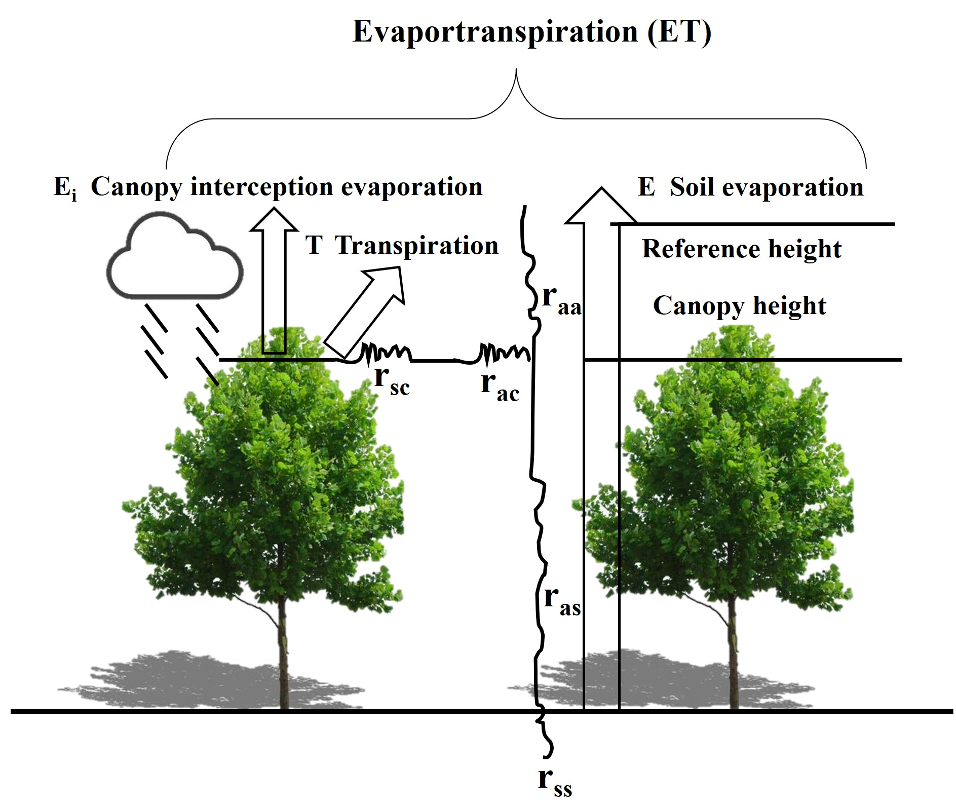
Figure 2 details the conceptual framework of the three-source model. In the improved SWH framework, total ecosystem ET ( λ E T , W m−2) is represented as the sum of T ( λ T ), E ( λ E ), and Ei ( λ E i ):
λ E T = λ T + λ E + λ E i = C c P M c 1 w f r + C s P M s + P M i w f r
P M c = R n G + ρ C p D r a c ( R n s G ) / r a a + r a c + γ 1 + r s c / ( r a a + r a c )
P M s = R n G + ρ C p D r a s ( R n R n s ) / r a a + r a s + γ 1 + r s s / ( r a a + r a s )
P M i = R n G + ρ C p D / r a a + r a s + γ
where P M c and P M s represent terms analogous to those in the original SWH model for estimating T and E, respectively. P M i is the P–M-type equation [22,26], which is canopy interception evaporation. It assumes zero canopy resistance in the P–M equation and employs an aerodynamic resistance defined as r a = r a a + r a s [20,26]. The canopy and soil surface resistances are given by C c and C s . The thermodynamic constants include the air density ( ρ , 1.293 kg m−3), the specific heat of air at constant pressure ( C p , 1012 J kg−1 K−1), and the psychrometric constant (γ, 0.067 kPa K−1). Additionally, reflects the slope of the saturation vapor pressure curve at a given air temperature (kPa K−1), while D captures the vapor pressure deficit (kPa).
Equation (1) defines the computation of the two coefficients, C c and C s , as follows:
C c = 1 1 + ρ c ρ a / ρ s ρ c + ρ a
C s = 1 1 + ρ s ρ a / ρ c ρ s + ρ a
where ρ a , ρ c , and ρ s are given by:
ρ a = + γ r a a
ρ c = + γ r a c + γ r s c
ρ s = + γ r a s + γ r s s
The resistances ( r a s ,   r a c , r a a ,   r s c ,   and   r s s ) are described in Section 2.4.
In Equations (2)–(4), the energy available to the canopy and the soil component is represented by R n and R n s , respectively. The soil surface radiation R n s is calculated via LAI based on Beer’s law [37]:
R n s = R n e x p L i g h t E x t C o e f × L A I
where R n refers to the net radiation energy incident on the canopy, with R n s representing that on the soil surface. The extinction coefficient ( L i g h t E x t C o e f ) was optimized in our model through a Monte Carlo–based approach.
In Equation (1), the wetted fraction of the canopy ( w f r ) [22,27,38] is calculated based on rainfall interception ( w r ) and canopy water-holding capacity ( w r m a x ) [29]:
p = δ × L A I
w r m a x = δ × L A I × ( 1 F P A R / L A I )
w r = P × 1 F P A R L A I P p w r m a x P > p
w f r = w r w r m a x 2 / 3
where p represents the critical half-hourly precipitation threshold. The parameter δ represents the maximum leaf water storage depth, which was also optimized using the Monte Carlo approach. w r m a x is the maximum canopy interception within a half-hour period, which is expressed as the function of LAI. FPAR, representing the proportion of PAR intercepted by vegetation, was derived as FPAR = 1 − exp(−LAI×LightExtCoef), and P is the rainfall above the canopy. To match daily flux tower observations, both p and w r m a x were subsequently converted to a daily timescale.

2.4. Estimation of Resistances Within the Enhanced SWH Model

The aerodynamic resistances rac, ras and raa, in Equations (7)–(9) were determined using the method described by Shuttleworth and Wallace [11]. Hu et al. [14] modified the parameterization of soil surface resistance ( r s s ) within the S–W framework, redefining it to be dependent on SW:
r s s = b 1 θ s θ b 2 + b 3
where θ is the volumetric SW (m3 m−3), and θ s is the saturated SW (0.42 for QYZ and 0.54 for DHS, empirically determined). b1 (s m−1), b2, and b3 (s m−1) are determined empirically, with b1 specified as 3.5 s m−1.
The canopy resistance ( r s c ) was calculated by applying the Ball–Berry model [39,40]:
r s c = 1 g 0 + a 1 P n h s / c a
where g 0 and a 1 are empirical constants. The term P n (µmol m−2 s−1) corresponds to the photosynthetic rate, which is approximated by GPP. h s and c a denote the leaf-surface relative humidity and CO2 concentration, respectively, with c a assigned a constant value of 390 ppm.
Furthermore, to better adapt the three-source framework to forest ecosystems, we modified the derivation of the displacement height ( d ) and roughness length ( z 0 ). These parameters, which are essential for determining aerodynamic resistances in the baseline SWH model, were updated in accordance with prior literature [22,41] as follows:
d = 0.75 × h
z 0 = 0.10 × h
where h was the canopy height.

2.5. Model Parameterization

The Monte Carlo technique was employed to optimize six empirical parameters (g0, b2, b3, a1, δ, and LightExtCoef), with the initial parameter ranges specified in Table S1 of the Supplementary Materials. Each parameter set was incorporated into the three-source model and evaluated against EC measurements from the QYZ (2004–2007) and DHS (2005–2007) sites. For each site, the first 50% of the complete time series was used for parameter calibration, while the remaining 50% was used for model validation. The predictive accuracy of the framework was evaluated via the R2 value to gauge the goodness of fit, alongside the regression slope (k) to assess potential bias. We retained the ten parameter sets that yielded the highest R2 values (mostly close to 1) and had k values between 0.99 and 1.01. These retained parameter sets were subsequently applied to the improved model, and the final ET estimates were obtained as the ensemble mean of these simulations to reduce uncertainty. The specific details of the Monte Carlo simulation are described in Hu et al. [14], and identical procedures and parameter ranges were applied for the SWH model as well.

3. Results

3.1. Validation of the Three-Source Model

A total of 10,000 Monte Carlo simulations were executed to isolate ten optimal parameter configurations, whose mean values were subsequently applied to parameterize the three-source framework (Table 2). The analytical outcomes demonstrate that the dual parameters, b3 and a1, together with the model-derived E/ET and T/ET ratios (∑E/∑ET and ∑T/∑ET), showed only minor variability. Furthermore, the relatively small standard deviations of most parameters indicate their stability. Notably, the standard errors of ∑E/∑ET were all 0.01, and that for ∑T/∑ET was below 0.01, highlighting the strong robustness of the three-source model in partitioning ET components. Furthermore, the three-source framework demonstrated reliable accuracy throughout the calibration phase, yielding R2 values of 0.93 and 0.85 at the QYZ and DHS sites, respectively, while both regression slopes converged near 1.0.

3.2. Performance of the Three-Source Model on Simulating ET

3.2.1. Overall Assessment

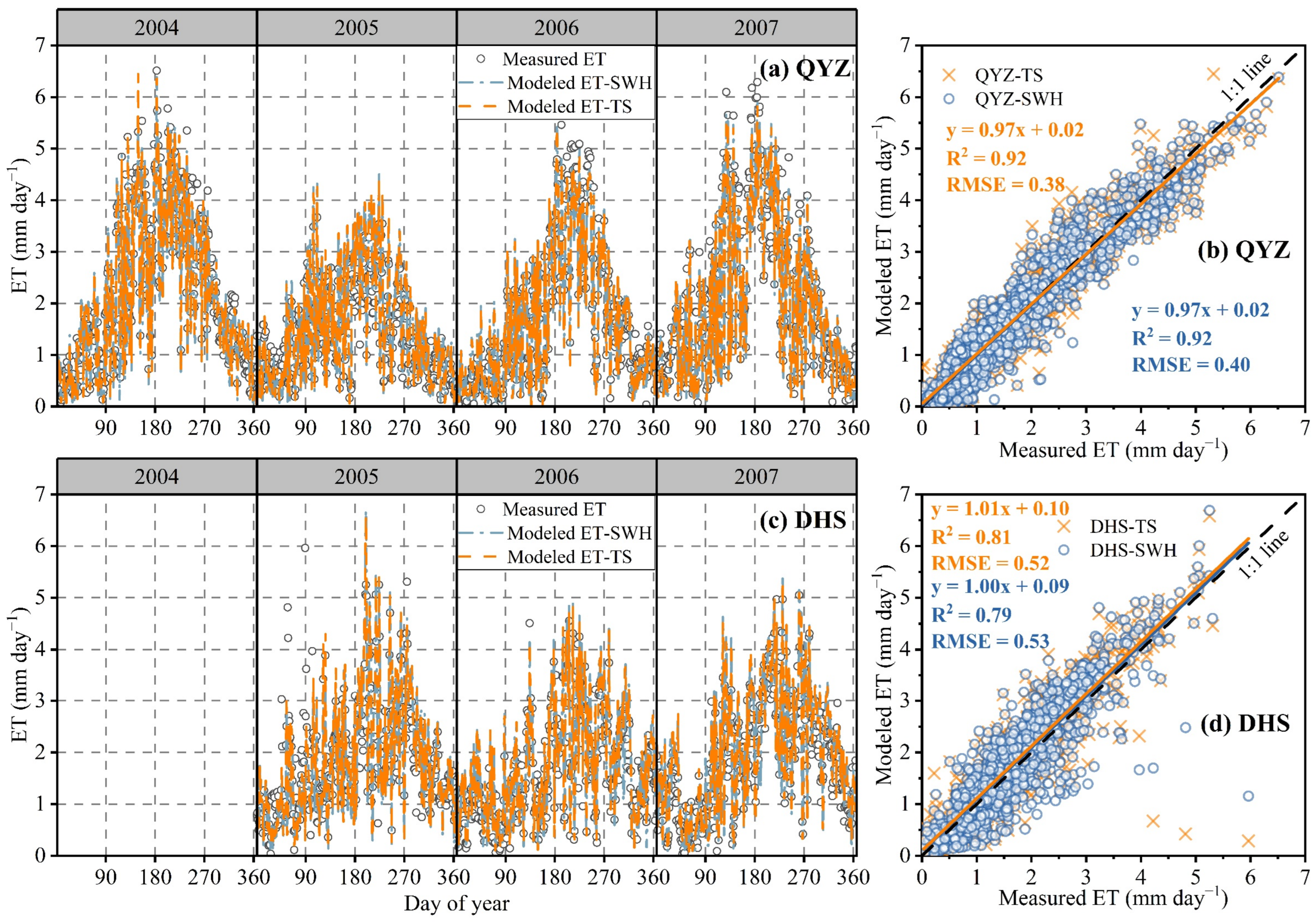
Using the three-source model and the SWH model, we simulated daily ET at the QYZ (2004–2007) and DHS sites (2005–2007) sites and compared the results with EC measurements (Figure 3). Overall, both models reproduced the observed ET reasonably well (Figure 3a,c). At QYZ (Figure 3b), the regression between modeled and observed ET yielded k values of 0.97 for both the three-source and SWH models. Both models achieved an R 2 of 0.92, with root mean square error (RMSE) values of 0.38 mm day−1 and 0.40 mm day−1, respectively, indicating strong performance of both models. By contrast, at DHS (Figure 3d), the three-source model achieved a slope of 1.01, R2 of 0.81, and RMSE of 0.52 mm day−1, while the SWH model showed relatively poorer performance with a slope of 1.00, R2 of 0.79, and RMSE of 0.53 mm day−1. These results suggest that the three-source model provides more accurate ET simulations at both sites, with the RMSE of ET simulations at the QYZ and DHS sites decreasing by 4.33% and 3.10%, respectively. In addition, the model performed well when validated on an extended dataset, which includes data from the QYZ station (2011–2015) and the Changbaishan mixed forest (CBS) site (2003–2006) (Supplementary Figure S1). This further confirms the performance and applicability of the three-source model.

3.2.2. Annual Assessment

At the QYZ station, annual validation of ET simulations by the three-source and SWH models against EC measurements indicated comparable performance (Table 3). Except for 2005—when both models overestimated ET, yielding k values of 1.31 and 1.32—their k values consistently ranged from 0.94 to 0.97. The corresponding R2 values were 0.92–0.94 for the three-source model and 0.91–0.93 for the SWH model. RMSEs ranged from 0.36 to 0.43 mm day−1 for the three-source model and from 0.36 to 0.44 mm day−1 for the SWH model. Importantly, the three-source model outperformed the SWH model, with annual RMSE reduction ranging from 1.66% to 7.85%. At the DHS station (Table 3), the three-source model yielded k values of 0.96–1.07 and R2 values of 0.71–0.87. In contrast, the SWH model produced k values of 0.97–1.04 and R2 values of 0.73–0.83, with RMSEs ranging from 0.47 to 0.60 mm day−1 compared to 0.45–0.62 mm day−1 for the three-source model. Although the SWH approach slightly outperformed the three-source model in 2005 due to interpolated missing rainfall data, the proposed framework demonstrated superior predictive capabilities in 2006 and 2007, with its RMSE decreasing by 6.21% and 10.68%, respectively, compared to the SWH baseline. Overall, across the years analyzed, the three-source model generally outperformed the SWH model in simulating ET.
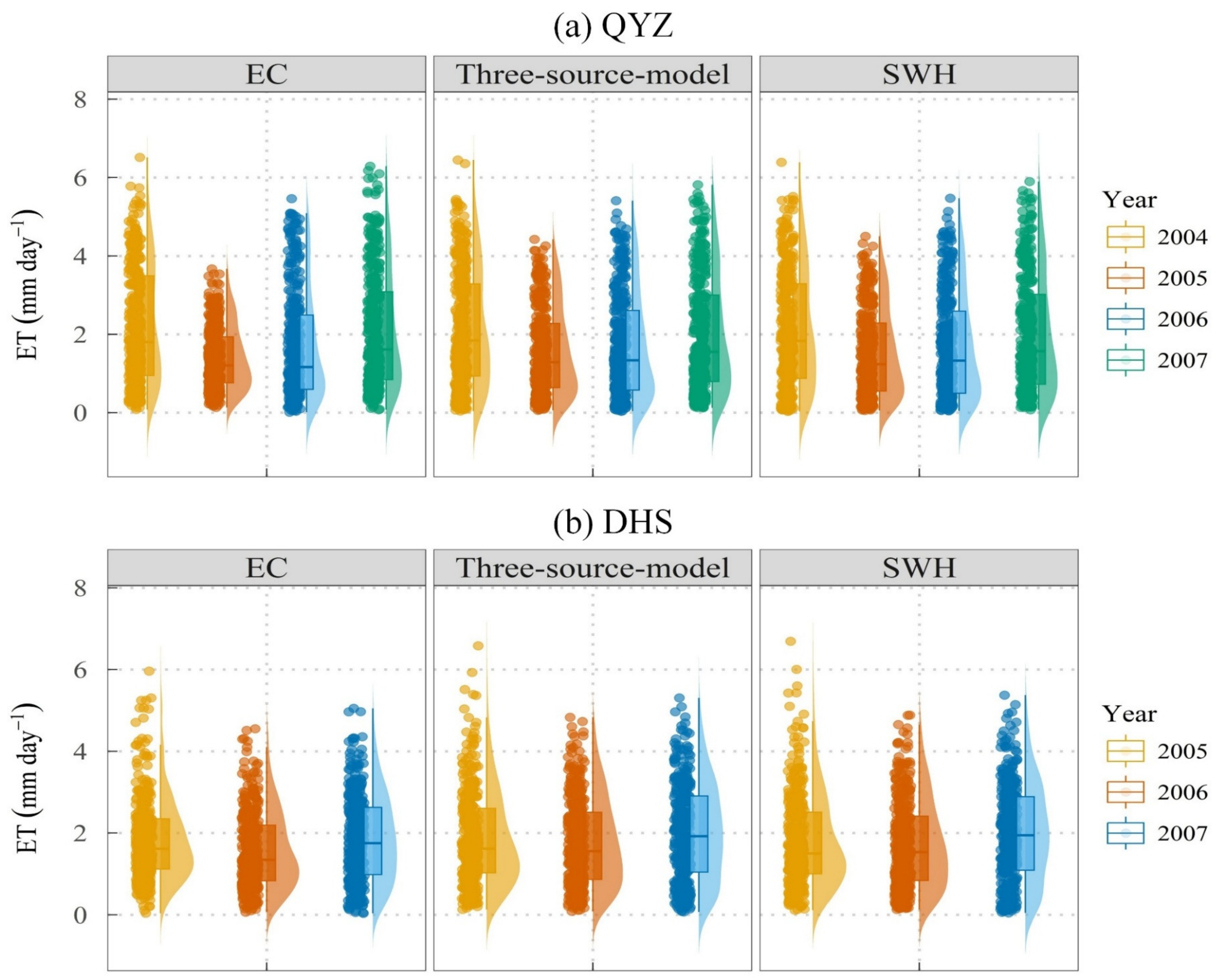
At the QYZ site (Figure 4a), ET measured by EC ranged from 0.012 to 6.514 mm day−1, while the three-source and SWH models simulated ranges of 0.036–6.445 mm day−1 and 0.032–6.388 mm day−1, respectively. The corresponding mean ET values were 1.847, 1.840, and 1.820 mm day−1, respectively. These results demonstrate that the three-source model produced estimates more consistent with EC observations than the SWH model. At the DHS site (Figure 4b), EC-measured ET ranged from 0.036 to 5.962 mm day−1, compared with 0.072–6.580 mm day−1 for the three-source model and 0.044–6.691 mm day−1 for the SWH model. The mean ET values were 1.756, 1.877, and 1.845 mm day−1, respectively. This suggests that both the three-source model and the SWH model slightly overestimated the ET at the DHS site during the observation period.

3.3. Estimate of Seasonal ET, T, E, and Ei

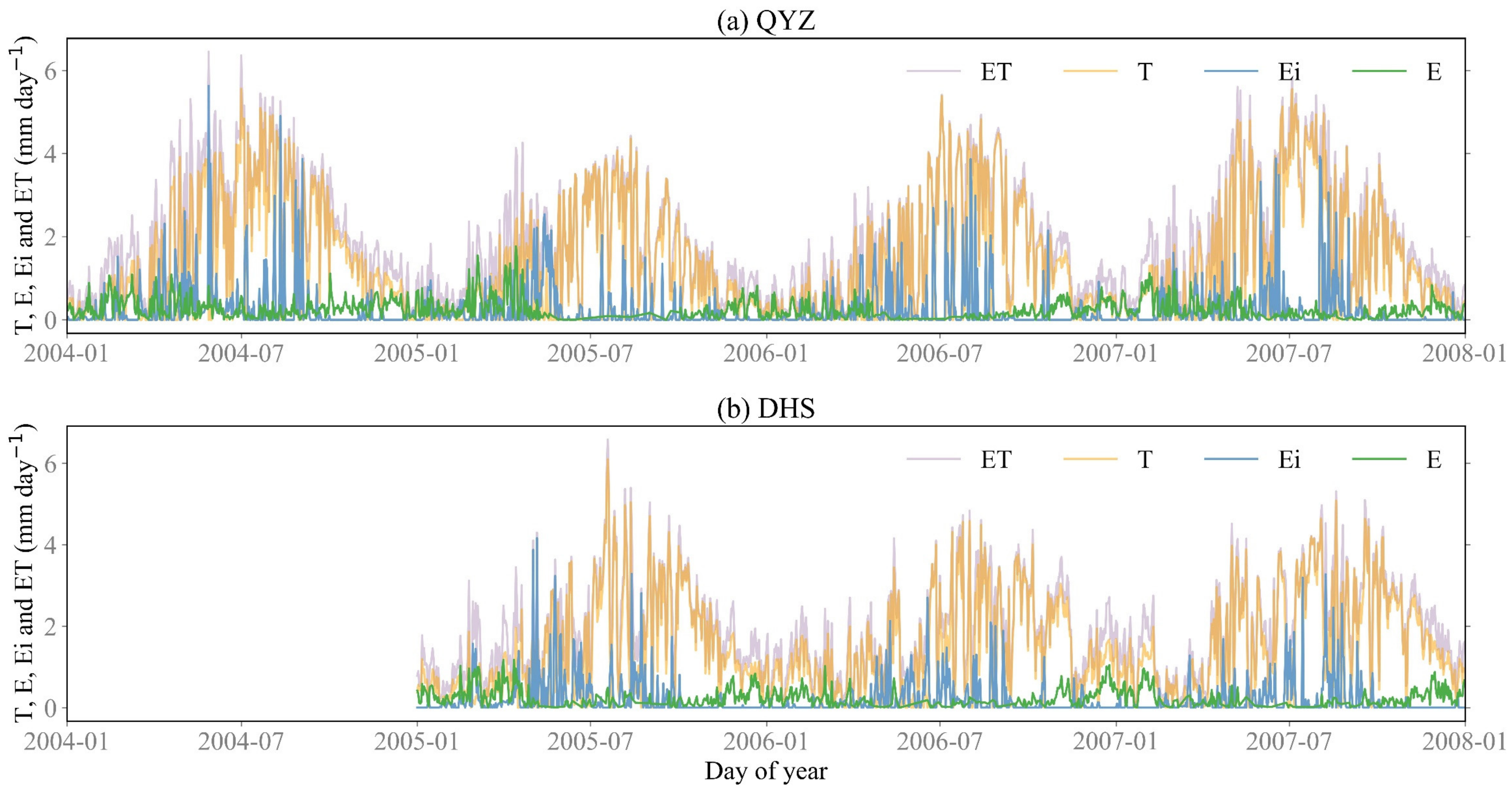
The seasonal dynamics of ET and its constituent fluxes at the QYZ (2004–2007) and DHS (2005–2007) sites are illustrated in Figure 5. Both sites exhibited clear unimodal seasonal trends for ET and T, with minima occurring in January and December, and maxima concentrated in June and July. In contrast, E remained low and relatively stable throughout the year, with average annual totals of 82.61 mm and 73.90 mm at QYZ and DHS, accounting for 12.29% and 10.79% of total ET, respectively. Ei was primarily concentrated during the peak rainfall season (April–September). Notably, at QYZ, which is influenced by the subtropical high-pressure system, midsummer droughts frequently occurred in July, leading to a marked reduction in precipitation and a sharp decline in Ei. Consequently, the seasonal variation of Ei demonstrated a distinct bimodal pattern. Overall, the seasonal patterns of ET and its components at both sites corresponded well to the results of Lu et al. [33].
Table 4 summarizes the simulated values of ET, E, T, Ei, and T/ET by the three-source model for both the entire year (months 1–12) and the growing season (months 5–9). Results showed that as canopy density increased, the contribution of T to ET also increased. At the QYZ site, where LAI rose from 1.94 to 2.22, the annual T/ET ratio increased from 72% to 77%, while the growing-season ratio increased from 78% to 83%, indicating that denser canopy cover promotes greater water loss through transpiration. By comparison, in the DHS ecosystem with a consistently high LAI, the difference in T/ET between the growing season and the entire year was only 1%–2%, whereas at the QYZ site with lower LAI it reached 6%–10%. These findings suggest that LAI is a fundamental determinant in regulating ecosystem water balance.

3.4. Spatiotemporal Characteristics of T/ET and the Underlying Controls

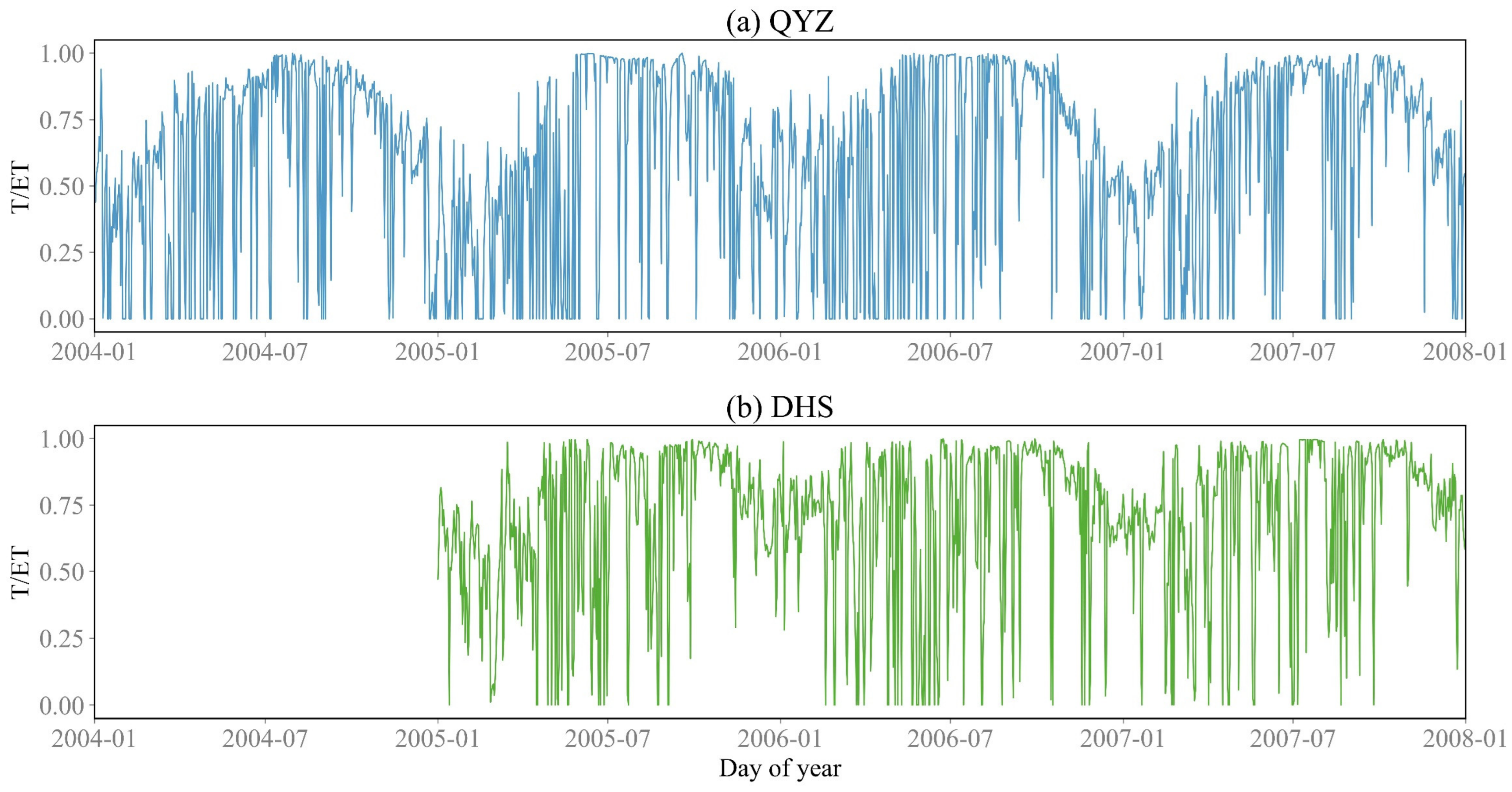
The daily variations of T/ET at the QYZ and DHS sites were modeled using the three-source model (Figure 6). From 2004 to 2007, approximately 70% of the daily T/ET values at QYZ fell within the ranges of 0.3–1.0. In contrast, from 2005 to 2007, nearly 70% of the daily T/ET values at the DHS site were greater than 0.6. During their respective study periods, T/ET dropped to zero on 216 days at QYZ and 61 days at DHS, accounting for 14.78% and 5.57% of the total data, respectively. These zero values primarily occurred during prolonged heavy rainfall, when intercepted water exceeded leaf storage capacity. Under such conditions, leaf surfaces were covered by a continuous water film, stomata closed, and transpiration was effectively suppressed, with all available energy allocated to Ei [42]. During the entire study period, when the daily T was 0, the daily cumulative Ei values at both sites accounted for 99% of the total Ei over the study period. Therefore, neglecting Ei in the model would introduce errors in ET partitioning, particularly during periods of continuous rainfall. [13,18,43]. At both sites, T/ET exhibited a predominantly unimodal seasonal pattern, characterized by elevated values during the growing season relative to the non-growing season, consistent with the 10-day moving average results reported by Zhu et al. [41]. During the growing season, dense canopy cover promoted T dominance, with T/ET approaching unity at both sites. In contrast, during the non-growing season, T/ET at DHS remained consistently higher than at QYZ. This contrast is most plausibly attributed to the reduced stomatal conductance in the QYZ coniferous plantation relative to the DHS evergreen broadleaf forest, thereby promoting higher T at DHS [44].
The Pearson correlation relationships between environmental factors and T/ET were quantified. As shown in Table 5, the temporal variations of T/ET at both QYZ and DHS were influenced by multiple factors, with generally consistent correlations across the two sites. Ta, VPD, Rn, and LAI all showed significant positive correlations with T/ET. Among these, VPD exhibited the strongest positive association, with correlation coefficients of 0.61 at QYZ and 0.55 at DHS, highlighting its pivotal role as a key environmental regulator of transpiration. In contrast, RH, SW, and Pre displayed significant negative correlations with T/ET. Pre had the strongest negative effect, with correlation coefficients of −0.63 (at QYZ) and −0.69 (at DHS), indicating its primary role in constraining transpiration efficiency.
Generally, T/ET tends to increase with vegetation coverage [23,45,46]. In this study, it was observed that LAI is positively correlated with T/ET (Table 5), but the correlation coefficient is not high. Similarly, Zhu et al. [41] reported no significant association between T/ET and LAI at these sites. Using the uWUE model, Cao et al. [23] showed that among 95 sites, only 4 exhibited significant correlations between annual T/ET and LAI (R2 = 0.56), whereas most sites were primarily regulated by climatic drivers, with R2 ranging from 0.25 to 0.33. These findings suggest that interannual variations in T/ET are governed by multiple interacting factors, and that vegetation structural attributes such as LAI play a secondary role compared with climatic controls.
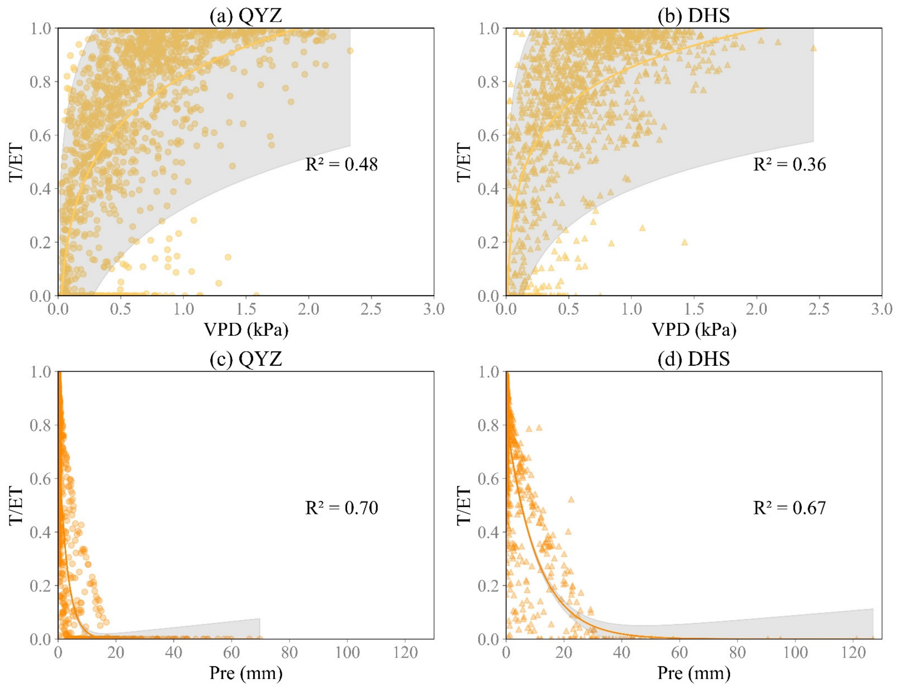
Figure 7 illustrates the relationships between daily T/ET and its two most influential factors, VPD and Pre. As VPD increased, T/ET showed a nonlinear upward trend (Figure 7a,b). When VPD reached approximately 2.0 kPa, T/ET tended toward 1.0 (mean R2 = 0.42), consistent with observations from subtropical sites reported by Cao et al. [23], as well as the multi-model results across 124 global sites presented by Nelson et al. [47]. This could be attributed to the concurrent increase in both VPD and LAI at the seasonal scale [48]. On one hand, an increase in LAI suppresses E via canopy shading while simultaneously increasing the transpiring leaf area to enhance T, jointly driving up the T/ET ratio. On the other hand, periods of high VPD are typically accompanied by clear and rainless weather. During these periods, Ei is minimal due to the lack of precipitation, and E declines rapidly as topsoil moisture depletes. In contrast, vegetation can access deep soil water through its roots, sustaining the continuous response of T to high atmospheric moisture demand, which further drives the steady rise of T/ET.
Pre exhibited a strong negative correlation with T/ET (Figure 7c,d), with a mean R2 = 0.685 consistent with previous findings [45,49,50]. In contrast, Schlesinger and Jasechko [51], based on 81 experimental and modeling studies that partitioned ET into E and T, reported only a weak association between Pre and T/ET. Gu et al. [45] further demonstrated that while increasing annual Pre significantly reduced T/ET (R2 = 0.205), the ratio of (T + Ei)/ET increased (R2 = 0.119). These findings indicate that excluding Ei from ET estimates can obscure the distinction between T and Ei, thereby increasing uncertainty in the response of T/ET to Pre. Incorporating Ei explicitly is thus essential for reliable assessments of forest water-use efficiency and ecohydrological stability. By resolving the contributions of T, E, and Ei under different climatic conditions, the three-source framework improves predictions of forest water dynamics under hydroclimatic variability and guides adaptive management to sustain ecosystem water and carbon balances.

4. Discussion

4.1. The Three-Source Model’s Performance in ET Simulation and Partitioning

Based on the SWH dual-source ET model, this study incorporated an Ei module without empirical parameters to construct a three-source model. The model achieved high accuracy in simulating ET at two subtropical forest sites. From 2004 to 2007, simulated ET yielded k values of 0.97 and 1.01, R2 of 0.92 and 0.81, and RMSE of 0.38 and 0.52 mm day−1 at QYZ and DHS, respectively, consistently outperforming the SWH model (Figure 3). In terms of mean absolute error (MAE), the three-source model also performed better (0.30 and 0.37 mm day−1) than the SWH model (0.31 and 0.40 mm day−1). The Diebold-Mariano (DM) test, using MAE as the loss function, further indicated that these differences are highly statistically significant. The DM statistics for the two sites were −6.25 and −7.52 (p < 0.001, lag order = 1), respectively, confirming that the prediction error of the three-source model in subtropical forest ecosystems is significantly lower than that of the SWH model. The slightly lower accuracy at DHS was primarily due to uncertainties from cloud- and rain-induced noise in remote sensing inputs (LAI) [24,33,52]. Importantly, the three-source model also outperformed the PT–JPL framework. Lu et al. [33] reported k values of 1.029 and 1.22, R2 of 0.75 and 0.50, and RMSE of 0.75 and 1.08 mm day−1 at QYZ and DHS from 2003 to 2008, respectively. These comparisons highlight that, unlike the PT-JPL Ei scheme incorporated into the SWH model by Cao et al. [23], which may introduce additional errors, the three-source model developed in this study substantially reduces uncertainties in ET simulations and improves reliability across subtropical forest ecosystems.
Table 6 shows clear differences in the annual T/ET simulated by the three-source and SWH models as well as the observed annual T/ET values. The average T/ET values at the QYZ and DHS stations from 2004 to 2006 were 0.77 and 0.72, respectively. over the course of the study the three-source model estimated mean T/ET values of 0.74 at QYZ and 0.79 at DHS, whereas the SWH model produced higher ratios of 0.85 and 0.87—over 0.08 greater. Ren et al. [44] simulated a T/ET ratio of 0.64 for a subtropical evergreen and deciduous broadleaf mixed forest using the PT-JPL model. Ren et al. [53] reported an average T/ET of 77.40% at the QYZ station using the Simplified Photosynthesis and Evapotranspiration model. Wei et al. [54] derived T/ET values ranging from 63% to 68% at the QYZ station from 2003 to 2008 using the PT-Fi remote sensing model. Shen et al. [21] obtained a T/ET value of 85% at the QYZ station in 2011 using the S–W model with an embedded Ei module, which set w r m a x as a fixed constant. In contrast, the Ei module in our study dynamically links w r m a x with LAI and is integrated into the SWH model, making it mechanistically more robust. The evidence from these studies suggests that the T/ET values simulated by both the three-source and SWH models are within a reasonable range, with the three-source model’s values being closer to the observed values than those from the SWH model. The higher ratios from the SWH model likely arise because it partitions ET into only E and T while neglecting Ei, thereby systematically overestimating T/ET [19,45].

4.2. Model Structure and Parameters

This study confirmed the accuracy of the three-source model in simulating and partitioning ET at the daily scale for two subtropical forest ecosystems. Overall, the proposed three-source model consistently outperformed the SWH baseline. This enhanced accuracy can primarily be attributed to the following three factors. (1) The inclusion of the Ei module in the SWH model allows for more accurate representation of the forest ecosystem during frequent rainfall events. This module quantifies the contribution of Ei to the total ET, effectively correcting the overestimation of T/ET caused by the neglect of Ei [13,19,43]. (2) The Ei module for simulating vegetation intercepted precipitation is more physically realistic [29]. Compared with the empirical interception formulas used in previous models [20,21,22], the formula in this study incorporates a critical precipitation threshold, which accounts for interception saturation as precipitation increases, effectively preventing overestimation during heavy rainfall. Additionally, the maximum interception capacity is not a fixed constant but is determined by key parameters such as LAI, vegetation coverage, and type, allowing the model to capture variations in interception capacity across different vegetation structures. (3) Key parameters were derived using Monte Carlo simulations. Unlike previous studies on precipitation interception estimation [22,30,31], where empirical values were often used for key parameters, potentially leading to significant deviations due to their site-specific nature, this study identified feasible parameter ranges through a series of steps prior to conducting the simulations [14], thus minimizing the uncertainty associated with parameter selection.
The average results based on the 10 optimal parameter sets show that the parameter values and their standard deviations at the QYZ site (b2 = 3.28 ± 1.00, b3 = 850.26 ± 74.49, a1 = 5.95 ± 0.34, g0 = 0.003 ± 0.001, LightExtCoef = 0.56 ± 0.042, δ = 0.11 ± 0.01) and the DHS station (b2 = 3.48 ± 0.78, b3 = 786.92 ± 82.91, a1 = 5.48 ± 0.20, g0 = 0.014 ± 0.001, LightExtCoef = 0.61 ± 0.03, δ = 0.12 ± 0.02) demonstrate that the parameter estimates are generally stable and fall within reasonable ranges [14,29,55,56]. From an ecological perspective, the higher b2 value at the DHS station suggests that soil moisture depletion has a stronger suppressive effect on soil evaporation in broadleaf forests. The higher b3 value at the QYZ station indicates that coniferous forests exhibit greater surface evaporation resistance when the soil is saturated. The higher a1 value at the QYZ station suggests that coniferous forests are more likely to support photosynthesis by increasing stomatal conductance. The g0 at the DHS site is slightly higher than that at the QYZ site, indicating that the artificial coniferous forest leaves at QYZ have a lower minimum stomatal conductance. This implies that these plants mitigate water loss by restricting the opening of their stomata. In contrast, the broadleaf forest leaves at the DHS site maintain a higher g0, with stomata remaining slightly open to ensure basic gas exchange. This is consistent with the results shown in Figure 6, where the T/ET at the DHS site is generally higher than at the QYZ site, further supporting the idea that plants at the DHS site adopt a more relaxed mechanism for water regulation. The higher LightExtCoef at the DHS station suggests that the canopy of broadleaf forests is denser, with lower light transmittance. The slightly higher δ value at the DHS station indicates that broadleaf leaves have a greater water-holding capacity. These differences in parameters reflect the ecological distinctions between the coniferous forest at QYZ and the broadleaf forest at DHS, which closely aligns with the observations reported by Ren et al. [44].

4.3. Research Contributions and Future Works

We developed a three-source model for simulating ET and its components, which demonstrated robust performance in two subtropical forest ecosystems. This study makes the following key contribution: Building upon the SWH model, a physically based Ei estimation module was embedded to form a three-source model. The framework of the SWH model and the P–M approach has seen widespread adoption across various ecosystems. The improvements to the wet fraction estimation module of the P–M equation provide a solid foundation for its broader applicability. Therefore, the three-source model theoretically holds significant potential for cross-ecosystem use. This study has preliminarily confirmed its reliability in forest ecosystems through empirical validation. However, to fully assess the model’s generalizability, further validation in other ecosystems, such as tropical rainforests, semi-arid woodlands, grasslands, farmlands, and wetlands, is needed. Additionally, while the historical flux tower datasets used in this study provided a solid baseline, they contained some missing values. Future research should utilize higher-quality, more up-to-date observational data to further test the model’s stability and applicability. Furthermore, due to the lack of in situ Ei measurements, this study followed previous research to indirectly validate the model’s ET partitioning performance using the T/ET ratio. Future studies should incorporate direct Ei observations (e.g., synchronous measurements of throughfall and stemflow) to further refine the model validation.

5. Conclusions

The present research formulated a three-source ET framework that partitions ET into T, E, and Ei. Validation against EC observations from the QYZ (2004–2007) and DHS stations (2005–2007) demonstrated that the model achieved RMSE values of 0.38 and 0.52 mm day−1, respectively, outperforming the SWH model (0.40 and 0.53 mm day−1). The annual mean T/ET simulated by the three-source model (0.74 at QYZ and 0.79 at DHS) was closer to the observed averages of approximately 0.77 and 0.72, respectively, compared to the values produced by the SWH model (0.85 and 0.87). The daily T/ET values of zero during continuous rainfall further highlight the limitations of the two-source model in partitioning ET. Among the environmental drivers, VPD showed a strong positive correlation with T/ET, while Pre exhibited a strong negative correlation. Overall, these results underscore the model’s potential to enhance assessments of ecosystem water resources and support adaptive management under a changing climate.

Supplementary Materials

The following supporting information can be downloaded at: https://www.mdpi.com/article/10.3390/f17080869/s1, Figure S1: Comparison of observed evapotranspiration (ET) via eddy covariance systems with modeled ET via three-source (TS) model and the SWH model at the Qianyanzhou subtropical coniferous plantation (QYZ) site (2011–2015) and Chang–Bai–Shan mixed forest (CBS) site (2003–2006). Note: There datasets were obtained from the China Ecosystem Research Network (CERN) (http://www.nesdc.org.cn/), and the overview of the CBS station can be found in the Zhu et al. (2015) [41]; Table S1: Parameters and their value ranges for Monte Carlo simulation. References [14,29,55,56] are cited in Supplementary Materials.

Author Contributions

Conceptualization, H.Z., L.X., M.T. and Y.L.; methodology, H.Z.; software, Q.Z.; validation, Q.Z.; formal analysis, H.Z.; investigation, Q.Z., M.T. and Y.L.; data curation, M.T., Y.L. and X.W.; writing—original draft preparation, H.Z.; writing—review and editing, L.X., M.T. and Y.L.; visualization, Q.Z.; funding acquisition, H.Z. and L.X. All authors have read and agreed to the published version of the manuscript.

Funding

This research was funded by the National Key R&D Program of China (2024YFE0106400), Jiangxi Province Key Laboratory of Watershed Ecological Process and Information (No. 2023SSY01052), State Key Laboratory of Lake and Watershed Science for Water Security (2024SKL003), the industry–university collaborative project between Zhejiang University of Water Resources and Electric Power and Jiangxi Xianwei Eco-Technology Co., Ltd. (No. H20250031), and its subsequent practice-oriented collaborative research, Science and Technology Program of Jiangxi Province (20244BCF61001, 20252BAC230006), and Project from Jiangxi Province (gpyc20250057).

Data Availability Statement

Data is contained within the article or Supplementary Material.

Acknowledgments

We gratefully acknowledge the helpful and constructive comments on the manuscript provided by the editors and anonymous reviewers.

Conflicts of Interest

Author Xingyuan Wu was employed by the company Jiangxi Xianwei Eco-Technology Co., Ltd. The remaining authors declare that the research was conducted in the absence of any commercial or financial relationships that could be construed as a potential conflict of interest.

References

  1. Jones, J.; Ellison, D.; Ferraz, S.; Lara, A.; Wei, X.; Zhang, Z. Forest restoration and hydrology. For. Ecol. Manag. 2022, 520, 120342. [Google Scholar] [CrossRef] [Scilit]
  2. Jasechko, S.; Sharp, Z.D.; Gibson, J.J.; Birks, S.J.; Yi, Y.; Fawcett, P.J. Terrestrial water fluxes dominated by transpiration. Nature 2013, 496, 347–350. [Google Scholar] [CrossRef] [Scilit] [PubMed]
  3. Jung, M.; Reichstein, M.; Ciais, P.; Seneviratne, S.I.; Sheffield, J.; Goulden, M.L.; Bonan, G.; Cescatti, A.; Chen, J.; De Jeu, R. Recent decline in the global land evapotranspiration trend due to limited moisture supply. Nature 2010, 467, 951–954. [Google Scholar] [CrossRef] [Scilit] [PubMed]
  4. Kim, W.; Woo, S.; Kim, S. Understanding the influence of increasing forest biomass on inter-annual evapotranspiration regime using the Budyko framework at forest-dominated landscape. Ecol. Indic. 2025, 174, 113508. [Google Scholar] [CrossRef] [Scilit]
  5. Oki, T.; Kanae, S. Global Hydrological Cycles and World Water Resources. Science 2006, 313, 1068–1072. [Google Scholar] [CrossRef] [Scilit] [PubMed]
  6. Walker, E.; Iannino, J.G.; Alonso, J.; Venturini, V. Effects of replacing natural grassland to Eucalyptus plantations on actual evapotranspiration using remote sensing data in Uruguay. For. Ecol. Manag. 2025, 593, 122861. [Google Scholar] [CrossRef] [Scilit]
  7. FAO. Global Forest Resources Assessment 2005: Progress Towards Sustainable Forest Management; FAO Forestry Paper: Rome, Italy, 2006; Volume 147, p. 320. [Google Scholar]
  8. Xu, M.; Ma, Q.; Li, S.; Yang, F.; Zhang, T.; Xu, F.; Yang, B.; Zhang, H.; Zhang, S.; Wang, Q.; et al. The estimation and partitioning of evapotranspiration in a coniferous plantation in subtropical China. Front. Plant Sci. 2023, 14, 1120202. [Google Scholar] [CrossRef] [Scilit] [PubMed]
  9. Fisher, J.B.; Whittaker, R.J.; Malhi, Y. ET come home: Potential evapotranspiration in geographical ecology. Glob. Ecol. Biogeogr. 2011, 20, 1–18. [Google Scholar] [CrossRef] [Scilit]
  10. Monteith, J.L. Evaporation and environment. Symp. Soc. Exp. Biol. 1965, 19, 205–234. [Google Scholar] [PubMed]
  11. Shuttleworth, W.J.; Wallace, J. Evaporation from sparse crops-an energy combination theory. Q. J. R. Meteorol. Soc. 1985, 111, 839–855. [Google Scholar] [CrossRef]
  12. Leuning, R.; Zhang, Y.Q.; Rajaud, A.; Cleugh, H.; Tu, K. A simple surface conductance model to estimate regional evaporation using MODIS leaf area index and the Penman-Monteith equation. Water Resour. Res. 2008, 44, W10419. [Google Scholar] [CrossRef] [Scilit]
  13. Hu, Z.; Li, S.; Yu, G.; Sun, X.; Zhang, L.; Han, S.; Li, Y. Modeling evapotranspiration by combing a two-source model, a leaf stomatal model, and a light-use efficiency model. J. Hydrol. 2013, 501, 186–192. [Google Scholar] [CrossRef] [Scilit]
  14. Hu, Z.; Yu, G.; Zhou, Y.; Sun, X.; Li, Y.; Shi, P.; Wang, Y.; Song, X.; Zheng, Z.; Zhang, L.; et al. Partitioning of evapotranspiration and its controls in four grassland ecosystems: Application of a two-source model. Agric. For. Meteorol. 2009, 149, 1410–1420. [Google Scholar] [CrossRef] [Scilit]
  15. Bao, Y.; Liu, T.; Duan, L.; Tong, X.; Zhang, L.; Singh, V.P.; Lei, H.; Wang, G. Comparison of an improved Penman-Monteith model and SWH model for estimating evapotranspiration in a meadow wetland in a semiarid region. Sci. Total Environ. 2021, 795, 148736. [Google Scholar] [CrossRef] [Scilit] [PubMed]
  16. Cui, Y.; Jia, L. A Modified Gash Model for Estimating Rainfall Interception Loss of Forest Using Remote Sensing Observations at Regional Scale. Water 2014, 6, 993–1012. [Google Scholar] [CrossRef] [Scilit]
  17. Zhong, F.; Jiang, S.; van Dijk, A.I.J.M.; Ren, L.; Schellekens, J.; Miralles, D.G. Revisiting large-scale interception patterns constrained by a synthesis of global experimental data. Hydrol. Earth Syst. Sci. 2022, 26, 5647–5667. [Google Scholar] [CrossRef] [Scilit]
  18. Hu, Z.; Wu, G.; Zhang, L.; Li, S.; Zhu, X.; Zheng, H.; Zhang, L.; Sun, X.; Yu, G. Modeling and Partitioning of Regional Evapotranspiration Using a Satellite-Driven Water-Carbon Coupling Model. Remote Sens. 2017, 9, 54. [Google Scholar] [CrossRef] [Scilit]
  19. Li, X.; Yang, Y.; Zhou, X.; Han, S.; Li, H.; Yang, Y.; Hao, X. Accuracy evaluation of ET and its components from three remote sensing ET models and one process based hydrological model using ground measured eddy covariance and sap flow. J. Hydrol. 2023, 626, 130374. [Google Scholar] [CrossRef] [Scilit]
  20. Iritz, Z.; Lindroth, A.; Heikinheimo, M.; Grelle, A.; Kellner, E. Test of a modified Shuttleworth–Wallace estimate of boreal forest evaporation. Agric. For. Meteorol. 1999, 98, 605–619. [Google Scholar] [CrossRef] [Scilit]
  21. Shen, J.; Zhang, M.; Xiao, W.; Wen, X.; Liu, S.; Li, X. Modeling evapotranspiration and its components in qianyanzhou plantation on modified SW model. Acta Ecol. Sin. 2016, 36, 2164–2174. (In Chinese) [Google Scholar] [CrossRef] [Scilit]
  22. Mo, X.; Liu, S.; Lin, Z.; Zhao, W. Simulating temporal and spatial variation of evapotranspiration over the Lushi basin. J. Hydrol. 2004, 285, 125–142. [Google Scholar] [CrossRef] [Scilit]
  23. Cao, R.; Huang, H.; Wu, G.; Han, D.; Jiang, Z.; Di, K.; Hu, Z. Spatiotemporal variations in the ratio of transpiration to evapotranspiration and its controlling factors across terrestrial biomes. Agric. For. Meteorol. 2022, 321, 108984. [Google Scholar] [CrossRef] [Scilit]
  24. Fisher, J.B.; Tu, K.P.; Baldocchi, D.D. Global estimates of the land–atmosphere water flux based on monthly AVHRR and ISLSCP-II data, validated at 16 FLUXNET sites. Remote Sens. Environ. 2008, 112, 901–919. [Google Scholar] [CrossRef] [Scilit]
  25. Choudhury, B.J.; Reginato, R.J.; Idso, S.B. An analysis of infrared temperature observations over wheat and calculation of latent heat flux. Agric. For. Meteorol. 1986, 37, 75–88. [Google Scholar] [CrossRef] [Scilit]
  26. Lhomme, J.P.; Montes, C. Generalized combination equations for canopy evaporation under dry and wet conditions. Hydrol. Earth Syst. Sci. 2014, 18, 1137–1149. [Google Scholar] [CrossRef] [Scilit]
  27. Noilhan, J.; Planton, S. A Simple Parameterization of Land Surface Processes for Meteorological Models. Mon. Weather Rev. 1989, 117, 536–549. [Google Scholar] [CrossRef] [Scilit]
  28. Yi, C.; Liu, K.; Zhou, T. Research on a formula of rainfall interception by vegetation. J. Soil Water Conserv. 1996, 2, 47–49. (In Chinese) [Google Scholar] [CrossRef] [Scilit]
  29. He, D.; Hong, W. Study of the improvement of formula of rainfall interception by vegetation. Syst. Sci. Compr. Stud. Agric. 1999, 15, 200–202. (In Chinese) [Google Scholar] [CrossRef] [Scilit]
  30. Lv, Y.; Liu, S.; Sun, P.; Liu, X.; Zhang, R. Canopy interception of sub-alpine dark coniferous communities in western Sichuan, China. Chin. J. Appl. Ecol. 2007, 18, 2398–2405. (In Chinese) [Google Scholar]
  31. Ma, W.; Ren, P.; Zeng, Y. The characteristics for the spatial-temporal evolution of water conservation value in farmland ecosystem in Chengdu Plain Economic Zone. China Land Sci. 2015, 29, 85–94. (In Chinese) [Google Scholar] [CrossRef] [Scilit]
  32. Zhang, N.; Liu, C. Simulated water fluxes during the growing season in semiarid grassland ecosystems under severe drought conditions. J. Hydrol. 2014, 512, 69–86. [Google Scholar] [CrossRef] [Scilit]
  33. Lu, Q.; He, H.; Zhu, X.; Yu, G.; Wang, H.; Zhang, J.; Yan, J. Study on the Variations of Forest Evapotranspiration and Its Components in Eastern China. J. Nat. Resour. 2015, 30, 1436–1448. (In Chinese) [Google Scholar]
  34. Xue, Z.; Chen, Y.; Yin, Y.; Chen, W.; Jiao, Y.; Deng, P.; Dai, S. Spatio-temporal characteristics and driving factors of flash drought in northern China from 1978 to 2020. Glob. Planet. Change 2024, 232, 104326. [Google Scholar] [CrossRef] [Scilit]
  35. Jönsson, P.; Eklundh, L. TIMESAT—A program for analyzing time-series of satellite sensor data. Comput. Geosci. 2004, 30, 833–845. [Google Scholar] [CrossRef] [Scilit]
  36. Yu, G.; Fu, Y.; Sun, X.; Wen, X.; Zhang, L. Recent progress and future directions of ChinaFLUX. Sci. China Ser. D. Earth Sci. 2006, 49, 1–23. [Google Scholar] [CrossRef] [Scilit]
  37. Beer, C.; Ciais, P.; Reichstein, M.; Baldocchi, D.; Law, B.E.; Papale, D.; Soussana, J.-F.; Ammann, C.; Buchmann, N.; Frank, D.; et al. Temporal and among-site variability of inherent water use efficiency at the ecosystem level. Glob. Biogeochem. Cycles 2009, 23, 1–13. [Google Scholar] [CrossRef] [Scilit]
  38. Deardorff, J.W. Efficient prediction of ground surface temperature and moisture, with inclusion of a layer of vegetation. J. Geophys. Res. Oceans 1978, 83, 1889–1903. [Google Scholar] [CrossRef] [Scilit]
  39. Ball, J.T.; Woodrow, I.E.; Berry, J.A. A Model Predicting Stomatal Conductance and its Contribution to the Control of Photosynthesis under Different Environmental Conditions. In Progress in Photosynthesis Research: Volume 4, Proceedings of the VIIth International Congress on Photosynthesis, Providence, RI, USA, 10–15 August 1986; Biggins, J., Ed.; Springer: Dordrecht, The Netherlands, 1987; pp. 221–224. [Google Scholar]
  40. Wang, Y.P.; Leuning, R. A two-leaf model for canopy conductance, photosynthesis and partitioning of available energy I:: Model description and comparison with a multi-layered model. Agric. For. Meteorol. 1998, 91, 89–111. [Google Scholar] [CrossRef] [Scilit]
  41. Zhu, X.-J.; Yu, G.-R.; Hu, Z.-M.; Wang, Q.-F.; He, H.-L.; Yan, J.-H.; Wang, H.-M.; Zhang, J.-H. Spatiotemporal variations of T/ET (the ratio of transpiration to evapotranspiration) in three forests of Eastern China. Ecol. Indic. 2015, 52, 411–421. [Google Scholar] [CrossRef] [Scilit]
  42. David, J.S.; Valente, F.; Gash, J.H. Evaporation of Intercepted Rainfall. In Encyclopedia of Hydrological Sciences; Anderson, M.G., Ed.; John Wiley & Sons, Ltd.: Chichester, UK, 2005; pp. 627–634. [Google Scholar]
  43. Mu, Q.; Zhao, M.; Running, S.W. Improvements to a MODIS global terrestrial evapotranspiration algorithm. Remote Sens. Environ. 2011, 115, 1781–1800. [Google Scholar] [CrossRef] [Scilit]
  44. Ren, X.; Lu, Q.; He, H.; Zhang, L.; Niu, Z. Estimation and analysis of the ratio of transpiration to evapotranspiration in forest ecosystems along the North-South Transect of East China. J. Geogr. Sci. 2019, 29, 1807–1822. [Google Scholar] [CrossRef] [Scilit]
  45. Gu, C.; Ma, J.; Zhu, G.; Yang, H.; Zhang, K.; Wang, Y.; Gu, C. Partitioning evapotranspiration using an optimized satellite-based ET model across biomes. Agric. For. Meteorol. 2018, 259, 355–363. [Google Scholar] [CrossRef] [Scilit]
  46. Fatichi, S.; Pappas, C. Constrained variability of modeled T:ET ratio across biomes. Geophys. Res. Lett. 2017, 44, 6795–6803. [Google Scholar] [CrossRef] [Scilit]
  47. Nelson, J.A.; Pérez-Priego, O.; Zhou, S.; Poyatos, R.; Zhang, Y.; Blanken, P.D.; Gimeno, T.E.; Wohlfahrt, G.; Desai, A.R.; Gioli, B.; et al. Ecosystem transpiration and evaporation: Insights from three water flux partitioning methods across FLUXNET sites. Glob. Change Biol. 2020, 26, 6916–6930. [Google Scholar] [CrossRef] [Scilit] [PubMed]
  48. Raghav, P.; Wagle, P.; Kumar, M.; Banerjee, T.; Neel, J.P.S. Vegetation Index-Based Partitioning of Evapotranspiration Is Deficient in Grazed Systems. Water Resour. Res. 2022, 58, e2022WR032067. [Google Scholar] [CrossRef] [Scilit]
  49. Moran, M.S.; Scott, R.L.; Keefer, T.O.; Emmerich, W.E.; Hernandez, M.; Nearing, G.S.; Paige, G.B.; Cosh, M.H.; O’Neill, P.E. Partitioning evapotranspiration in semiarid grassland and shrubland ecosystems using time series of soil surface temperature. Agric. For. Meteorol. 2009, 149, 59–72. [Google Scholar] [CrossRef] [Scilit]
  50. Loik, M.E.; Breshears, D.D.; Lauenroth, W.K.; Belnap, J. A multi-scale perspective of water pulses in dryland ecosystems: Climatology and ecohydrology of the western USA. Oecologia 2004, 141, 269–281. [Google Scholar] [CrossRef] [Scilit] [PubMed]
  51. Schlesinger, W.H.; Jasechko, S. Transpiration in the global water cycle. Agric. For. Meteorol. 2014, 189–190, 115–117. [Google Scholar] [CrossRef] [Scilit]
  52. Wu, G.; Hu, Z.; Li, S.; Zheng, H.; Zhu, X.; Sun, X.; Yu, G.; Li, J. Evaluation and uncertainty analysis of a two-source evapotranspiration model. Acta Geogr. Sin. 2016, 71, 1886–1897. (In Chinese) [Google Scholar]
  53. Ren, X.; He, H.; Moore, D.J.P.; Zhang, L.; Liu, M.; Li, F.; Yu, G.; Wang, H. Uncertainty analysis of modeled carbon and water fluxes in a subtropical coniferous plantation. J. Geophys. Res. Biogeosci. 2013, 118, 1674–1688. [Google Scholar] [CrossRef] [Scilit]
  54. Wei, H.; He, H.; Liu, M.; Zhang, L.; Yu, G.; Min, C.; Wang, H.; Liu, Y. Modeling evapotranspiration and its components in Qianyanzhou plantation based on remote sensing data. J. Nat. Resour. 2012, 27, 778–789. (In Chinese) [Google Scholar]
  55. Barnard, D.M.; Bauerle, W.L. The implications of minimum stomatal conductance on modeling water flux in forest canopies. J. Geophys. Res. Biogeosci. 2013, 118, 1322–1333. [Google Scholar] [CrossRef] [Scilit]
  56. Zhang, L.; Hu, Z.; Fan, J.; Zhou, D.; Tang, F. A meta-analysis of the canopy light extinction coefficient in terrestrial ecosystems. Front. Earth Sci. 2014, 8, 599–609. [Google Scholar] [CrossRef] [Scilit]
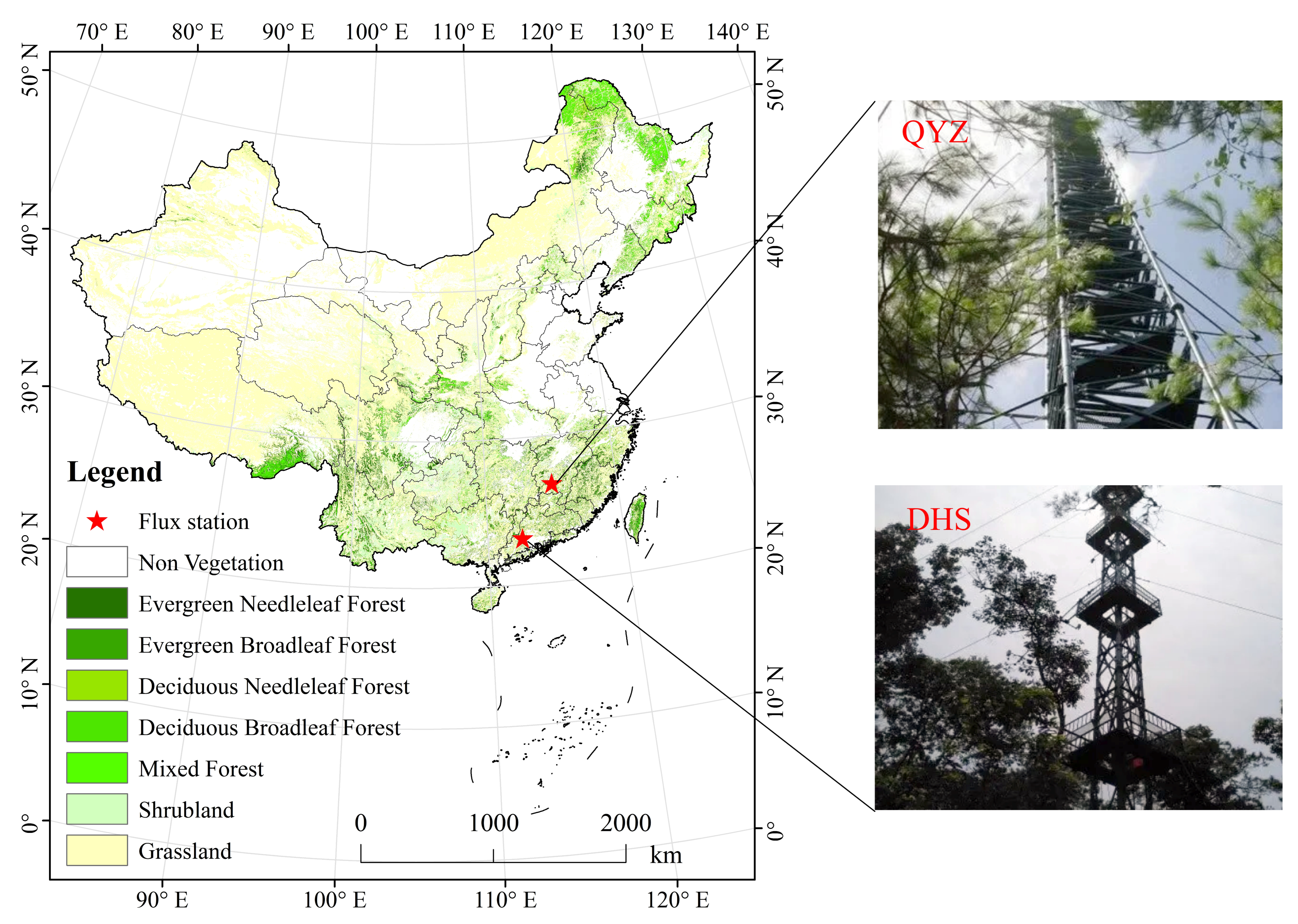
Figure 1. Geographical locations of QYZ and DHS.
Forests 17 00869 g001
Figure 2. Schematic diagrams of the three-source model.
Forests 17 00869 g002
Figure 3. Daily ET modeled by the three-source (TS) model and the SWH model with EC-measured values at the QYZ site (a,b) and DHS site (c,d). Note: SWH and TS denote the SWH model and the three-source model, respectively.
Forests 17 00869 g003
Figure 4. Interannual variations in daily ET modeled by the EC measurement, three-source model, and SWH model at the QYZ site (2004–2007) and DHS sites (2005–2007).
Forests 17 00869 g004
Figure 5. Seasonal variations in ET, T, E, and Ei at the QYZ and DHS stations.
Forests 17 00869 g005
Figure 6. Daily variation of T/ET at QYZ and DHS, respectively.
Forests 17 00869 g006
Figure 7. Effect of VPD and Pre on T/ET at QYZ and DHS, respectively. Note: The shaded area in the figure represents the 95% confidence interval.
Forests 17 00869 g007
Table 1. Station Overview.
StationQYZDHS
Latitude (°N)26.7323.17
Longitude (°E)115.05112.53
Altitude (m)100300
Climate typeSubtropical monsoon climate
Mean annual air temperature (°C)17.921.0
Mean annual total rainfall (mm)14851956
Canopy height(m)1222
Leaf area index (m2 m−2)3.54
Soil typeRed soilLatosolic red soil
Table 2. Ranges and mean values (sd) for both the parameters and the flux ratios (∑E/∑ET and ∑T/∑ET). Values enclosed in parentheses represent the standard deviations derived from simulations using the top 10 optimal parameter configurations.
Parameter and Value QYZDHS
b2Range1.66–4.382.21–4.70
Mean (sd)3.28 (1.00)3.48 (0.78)
b3Range668.62–912.89612.03–874.15
Mean (sd)850.26 (74.49)786.92 (82.91)
a1Range5.36–6.495.28–5.87
Mean (sd)5.95 (0.34)5.48 (0.20)
g0Range0.002–0.0050.013–0.015
Mean (sd)0.003 (0.001)0.014 (0.001)
LightExtCoefRange0.48–0.620.56–0.67
Mean (sd)0.56 (0.042)0.61 (0.03)
δRange0.10–0.130.10–0.18
Mean (sd)0.11 (0.01)0.12 (0.02)
kRange0.99–0.990.99–1.01
Mean (sd)0.99 (0.001)1.00 (0.01)
R2Range0.93–0.930.85–0.85
Mean (sd)0.92 (0.0001)0.85 (0.0009)
∑E/∑ETRange0.09–0.130.07–0.09
Mean (sd)0.11 (0.01)0.08 (0.01)
∑T/∑ETRange0.78–0.790.76–0.78
Mean (sd)0.79 (0.002)0.77 (0.008)
Table 3. Performance of the SWH model and three-source model.
SiteYearkR2RMSE
Three-Source ModelSWHThree-Source ModelSWHThree-Source ModelSWH
QYZ20040.970.970.940.930.360.40
20051.311.320.920.910.430.44
20060.940.940.930.930.350.36
20070.950.960.940.930.380.40
DHS20050.960.970.710.730.620.60
20061.071.040.860.830.450.47
20071.041.010.870.820.460.52
Table 4. Comparison of mean annual LAI ( L A I m e a n ), simulated ET ( E T m o d ), simulated E ( E m o d ), simulated T ( T m o d ), simulated Ei ( E i m o d ), and T m o d / E T m o d across full years and growing seasons.
SiteYear L A I m e a n All Year Around (1–12)Growing Season (5–9)
E T m o d E m o d T m o d E i m o d T / E T m o d E T m o d E m o d T m o d E i m o d T / E T m o d
QYZ20041.94777.76104.35563.00110.410.72506.1031.46394.6180.020.78
20051.95567.6782.12406.8678.700.72343.0212.58280.7749.660.82
20062.02611.7562.51462.0987.160.76401.2011.37332.0057.830.83
20072.22730.5281.46559.7789.280.77466.5419.88385.5261.140.83
Mean2.03671.9282.61497.9391.390.72429.2118.82348.2262.170.81
DHS20053.35676.7885.73498.2292.830.74370.8917.26281.3072.330.76
20063.35643.7468.76505.6369.350.79339.5315.43269.2954.820.79
20073.56734.4767.21597.7269.540.81410.6613.61341.3955.650.83
Mean3.41685.0073.90533.8677.240.78373.6915.43297.3360.930.79
Table 5. Correlation between T/ET and its drivers.
SiteTaRHVPDSWRnPreLAI
QYZ0.51 **1−0.51 **0.61 **−0.16 **0.57 **−0.63 **0.49 **
DHS0.30 **−0.39 **0.55 **−0.10 **0.48 **−0.69 **0.20 **
1 ** p < 0.01.
Table 6. The simulated annual T/ET in QYZ and DHS.
Models and ReferencesSite2004200520062007Mean
Three-source-modelQYZ0.720.720.760.770.74
DHS/0.760.790.830.79
SWH modelQYZ0.830.830.880.860.85
DHS/0.850.870.880.87
Two layer eddy covariance measured water vapor fluxes [41]QYZ0.850.690.77/0.77
DHS0.730.700.72/0.72
Disclaimer/Publisher’s Note: The statements, opinions and data contained in all publications are solely those of the individual author(s) and contributor(s) and not of MDPI and/or the editor(s). MDPI and/or the editor(s) disclaim responsibility for any injury to people or property resulting from any ideas, methods, instructions or products referred to in the content.