Article

Predicting Timber Board Foot Volume Using Forest Landscape Model and Allometric Equations Integrating Forest Inventory Data

1
Institute for Data Science and Informatics, University of Missouri, Columbia, MO 65211, USA
2
School of Natural Resources, Institute for Data Science and Informatics, University of Missouri, Columbia, MO 65211, USA
3
Northern Research Station, USDA Forest Service, Columbia, MO 65201, USA
*
Authors to whom correspondence should be addressed.
Forests 2025, 16(3), 543; https://doi.org/10.3390/f16030543
Submission received: 8 February 2025 / Revised: 16 March 2025 / Accepted: 17 March 2025 / Published: 19 March 2025

Abstract

:
In this study, we present a methodology for predicting timber board foot volume using a forest landscape model, incorporating allometric equations and forest inventory data. The research focuses on the Ozark Plateau, a 48,000-square-mile region characterized by productive soils and varied precipitation. To simulate timber volume, we used the LANDIS PRO forest landscape model, initialized with forest composition data derived from the USDA Forest Service’s Forest Inventory and Analysis (FIA) plots. The model accounted for species-specific growth rates and was run from the year 2000 to 2100 at five-year intervals. Timber volume estimates were calculated using both quadratic mean diameter (QMD) and tree diameter in the Hahn and Hansen board foot volume equation. These estimates were compared across different forest types—deciduous, coniferous, and mixed stands—and verified against FIA plot data using a paired permutation test. Results showed high correlations between QMD and tree diameter methods, with a slightly lower volume estimate from the QMD approach. Projections indicate significant increases in board foot volume for key species groups such as red oak and white oak while showing declines toward the end of the model period in groups like shortleaf pine due to age-related mortality and regeneration challenges. The model’s estimates closely align with state-level FIA data, underscoring the effectiveness of the integrated approach. The study highlights the utility of integrating landscape models and forest inventory data to predict timber volume over time, offering valuable insights for forest management and policy planning.

1. Introduction

Accurate estimation of timber volume is necessary for ecological analysis, economic forecasting, and forest management planning. More recent methods for estimating board foot volume include satellite imagery, which uses high-resolution images from satellites like Landsat and Sentinel-2 to estimate forest cover and biomass [1]. These estimates can be converted to timber volume using allometric equations [2]. Synthetic Aperture Radar sensors penetrate cloud cover and provide data on forest structure and biomass, which can be used to estimate timber volume [3]. Lidar data can be collected with manned or unmanned aircraft or from the ground, and laser pulses can be used to create high-resolution, three-dimensional maps of forest structures. LiDAR data can be used to estimate tree height, canopy structure, and biomass, which are critical for calculating timber volume [4,5].
More traditional methods use equations with inputs like diameter at breast height (DBH) and tree height to measure volume. Taper functions describe the shape of the tree trunk and are used to calculate the volume of the tree bole. Various taper equations have been developed for different tree species and regions [6]. While these methods can be used at the stand or tree scale, they may be more difficult to apply at a landscape scale or used to estimate board foot volume over time. Moreover, field and airborne-based methods are limited in forecasting timber volume over time.
Forest landscape models simulate the growth and succession of individual tree species based on their traits, such as shade tolerance, longevity, and dispersal abilities. This detailed representation allows the model to capture the dynamics of mixed-species forests and predict changes in species composition over time [7,8,9]. The models operate on a raster-based landscape, where each cell represents a specific area of the forest. Tree species and their respective age cohorts are tracked within each cell, allowing the model to simulate forest dynamics and the spread of disturbances across the heterogeneous landscape [9]. The models allow for the incorporation of different forest management strategies, including thinning, clear-cutting, and selective harvesting. By simulating these practices, forest landscape models help forest managers evaluate the long-term impacts of different management scenarios on forest structure, composition, and function [10].
Landscape modeling has increasingly become forward-looking. The source “Northern Forest Futures” ref. [11] is a comprehensive examination of the future of northern U.S. forests, considering various social, economic, and environmental factors. This work is part of the larger effort to understand how these forests are likely to change over the next several decades, providing insights for policymakers, forest managers, and the public. Human activities, such as land development, forest management, and recreational use, are becoming subjects of temporal examination. Topics include how economic trends, population growth, and changes in land ownership patterns will influence forest landscapes. For example, urban expansion and increased recreational use could lead to habitat fragmentation and changes in forest management priorities [12]. All these analyses benefit from understanding how sawlog volume changes over time. Thus, a method for modeling sawlog volume spatially and temporally is needed to understand how climate, management, and disease will impact forest inventory in the future. The purpose of this study is to (1) present a methodology to derive timber volume for forest landscape model simulation outcome, (2) verify the derived timber volume against forest inventory data, and (3) explore the current trends of timber volume for the westernmost central hardwood forests.

2. Materials and Methods

2.1. Study Area

The study area is the Ozark Plateau, which covers portions of southern Missouri, northern Arkansas, and northeast Oklahoma. The plateau covers approximately 48,000 square miles of mid-latitude temperate climate. Precipitation ranges from 38 inches per year in the north to 48 inches per year in the southern region of the study area. Alfisols and utensils are the dominant soil types and are generally very productive soils for agriculture and timber. Surface water is abundant in the study area, with several major rivers flowing radially away from the central part of the Ozark Plateau [13].

2.2. Model Parameterization and Simulation

Dijak et al. [14] created a 10-landform map for the region using the topographic index methods described by Jenness [15]. That map was sent to the USDA Forest Service, where Forest Inventory and Analysis (FIA) plot locations were intersected with the landform map, and plots were assigned a landform value filtering out plots where locations could be determined by the landform map. A total of 7591 plots were returned with landform values assigned [16]. The FIA plot data also contain the ecological subsection where each plot is located, as well as the plot’s site index. From the plot data, the mean site index was calculated for each combination of ecological subsection and landform, and the mean site index was assigned to a map by ecological subsection and landform. This information was used in conjunction with a satellite-based land cover map to derive the forest composition map using the Landscape Builder software [17]. The forest composition map was used to initialize the LANDIS Pro simulation.
The model period began with year zero in the year 2000 and ended with year 100 in 2100, modeled at 5-year increments. Basal area and tree number from LANDIS output rasters for each time step were used for the board foot volume calculation. Initial forest conditions were developed for the year 2000 by stochastically assigning a representative FIA plot to each raster cell based on land cover, landform, and size class from 1995 to 2005 FIA data. Parameters such as species growth rate and age-DBH relationship were iteratively adjusted in Landscape Builder until LANDIS Pro simulation results at year zero did not differ from FIA data for the year 2000 in ecological sections using mean basal area and density. A chi-square test was used to measure each iteration until there was no statistically significant difference between the model and FIA data. Growth rates and age-DBH relationships are, therefore, representative of observed climate parameters. Alternative climate scenarios were not tested. Harvest was simulated at existing volumes based on FIA management unit harvest information from 1995–2005 [18]. The species included were American elm (Ulmus americana), black cherry (Prunus serotina), loblolly pine (Pinus taeda), mockernut hickory (Carya tomentosa), northern red oak (Quercus rubra), post oak (Quercus stellata), red maple (Acer rubrum), shortleaf pine (Pinus echinata), southern red oak (Quercus falcata), sugar maple (Acer saccharum), sweet gum (Liquidambar styraciflua), white ash (Fraxinus americana), white oak (Quercus alba), and yellow poplar (Liriodendron tulipifera).

2.3. Board Foot Volume Calculation and Verification

Board foot volume was estimated for each pixel with a quadratic mean diameter greater than 5 inches. Quadratic mean diameter was calculated taking the following form [19]:
Q M D = B A N   0.005454
where BA is the total basal area and N is the number of stems.
International ¼ inch rule board foot volume estimates were calculated using a gross volume board foot equation [20] as follows:
V g r o s s = b 1 S b 2 1 e b 3 D b 4
where S is the site index, and D is the diameter of the tree, beta values are species-specific and come from Hahn and Hansen estimates.
To test the use of quadratic mean diameter in the Hahn and Hansen equation, gross board foot volume was modeled in 2639 FIA plots sampled from Arkansas, Illinois, Kansas, Missouri, and Oklahoma. We selected the 10 most common tree species that make up over 90% of forest biomass: black oak, loblolly pine, mockernut hickory, northern red oak, post oak, red maple, shortleaf pine, Shumard oak, southern red oak, and white oak. Plots were classified by percent basal area of coniferous species into coniferous, mixed, and deciduous plots, with less than 25% coniferous being classified as deciduous, 25%–50% coniferous being mixed, and greater than 50% coniferous being classified as coniferous. Minimum diameters of 9 inches for coniferous and 11 inches for mixed and deciduous plots were used. Board foot volume per acre was modeled for each group using both tree diameter and quadratic mean diameter of the plot using the Hahn and Hansen equation. A paired permutation means test was then conducted using 10,000 bootstrapped samples from the diameter and quadratic mean diameter board foot volumes to compare the means of board foot volumes calculated using the tree diameter and the quadratic mean diameter of the plot [21].

3. Results

The paired permutation test yielded a p-value of 1 for deciduous, mixed, and coniferous plots. The number of plots for coniferous, deciduous, and mixed forest were 771, 1724, and 144 plots, respectively. Plots containing only one tree were removed before the analysis, as the QMD would equal the Diameter. The mean absolute difference for the coniferous, deciduous, and mixed groups of FIA data were 76.21, 54.60, and 75.00 board feet per acre, respectively.
The mean board foot volume by plot for coniferous was 1521.95 for the diameter calculation, while the QMD volume was 1445.75 board feet. The deciduous group had a mean diameter volume of 1645.21 board feet and a QMD mean volume of 1591.42 board feet per acre. The mixed group showed a mean board foot volume per acre of 2040.19 with tree diameter and 1965.00 board feet per acre for the QMD calculation. The Pearson correlation coefficients rounded to 1 for all three groups, each with a p-value of 0. The correlation coefficients and p-values indicate a near-linear relationship between the two methods for calculating the Hahn and Hansen board foot volume equation (Figure 1). The relationship between the two methods is nearly linear. In each grouping, including the total, the board foot volume per acre using the QMD method was slightly less than using the Volume method.

3.1. The Red Oak Group

The red oak group included black oak, northern red oak, and southern red oak. In the year 2000, the Red Oak group starts with 26 billion board feet and an average of 1453 board feet per acre. There is an increasing trend in board foot volume throughout the first three-quarters of the century, with 2025 showing 2925 board feet per acre, with a peak around 2075 at 6194 board feet per acre (Figure 2 and Figure 3). There is a slight decrease finishing in 2100 with 100.4 billion board feet on the landscape and 5613 board feet per acre.

3.2. The White Oak Group

The modeled species in the white oak group are white oak and post oak. The white oak group shows a steady increase throughout the model, beginning with 35 billion board feet and 1956 board feet per acre in the year 2000. The year 2025 has the group increasing to 67 billion board feet and 3766 board feet per acre. The year 2075 shows 149 billion board feet in the landscape and 8338 board feet per acre. In 2100, the number increased to 174 billion board feet and 9766 per acre (Figure 3 and Figure 4).

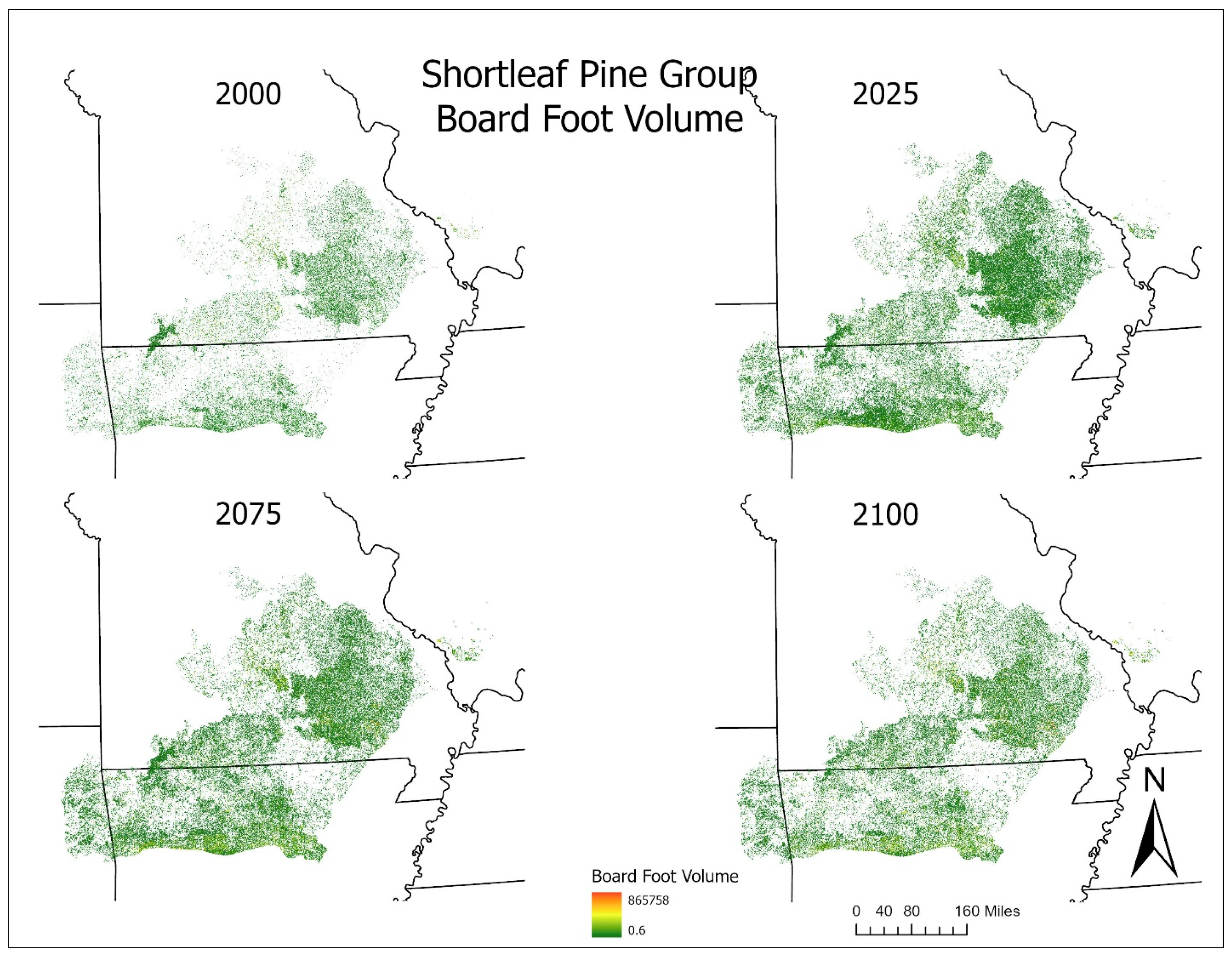
3.3. Shortleaf Pine Group

The shortleaf pine group includes shortleaf and loblolly Pine. This group is modest compared to the oak groups, but it is still a commercially viable group. The model begins with 7 billion board feet in the landscape and 411 board feet per acre. Growth in the first 25 years increases the group to 774 board feet per acre. The increase continues, and 2075 shows 1022 board feet per acre, but there is a slight decline toward the end of the century, finishing with 17 billion board feet in the landscape and 964 board feet per acre (Figure 3, Appendix A).

3.4. The Complete Model

The complete model contains 13 species, including the previously discussed groups and other hardwood species like black cherry, mockernut hickory, sugar maple, American elm, and white ash. The model starts with 72 billion board feet on the landscape and quickly increases to 151 billion board feet in 2025. It continues to grow with 341 billion board feet in 2075 and finishes with 376 billion board feet in 2100. The model shows 21,047 board feet per acre in 2100 (Figure 5).
The Missouri summary includes a greater number of species (n = 89) than what is currently parameterized in the LANDIS model (i.e., n = 13). We can, however, compare individual species contained in the LANDIS model in the year 2020 with those in the Missouri summary for timberland. The percent difference between model estimates and FIA was calculated. Many of the oak species had a percent difference of less than −20%. The largest percentage differences occur when the cubic foot estimates are the lowest, and minor differences can lead to considerable percentage variations (Figure 5).

4. Discussion

A p-value of 1 in the paired permutation test indicates that every possible permutation of the data is equally likely to produce a test statistic as extreme or more extreme than the observed test statistic [22]. A 2021 report on the condition of Missouri forests using data collected from 2013 through 2018 shows that approximately 65% of oak species are of large diameter, indicating an older age class. The decline of the red oak group toward the end of the century is indicative of age-related mortality of larger diameter trees within the group as the group declines and regenerates [23]. At its peak in 2075, the red oak group shows the most volume in the north-central and southern regions of the study area, with more sparse coverage in the western and northwestern regions, in addition to areas east of the Mississippi River. For the white oak group, the overall trend is a sharper increase in the first half of the century, followed by a slowing rate of volume growth throughout the last half of the century. The 2021 report from FIA shows that shortleaf pine forests are approximately 84% large in diameter, so the end of the century shows some decline from mortality within the group with relatively poor regeneration [23]. The white oak group appears to be overtaking both the red oak and shortleaf pine groups toward the end of the 21st century.
All the LANDIS board foot estimates except for red maple were less than the FIA board foot estimates. There are two factors contributing to this difference. The first is that the LANDIS model uses NLCD landcover classifications, which can contain marginally productive soils that yield less timber. The FIA data were collected from what is classified as timberland, which can contain more productive soils than the average soil quality found in the landscape. To illustrate this, the total timberland that was surveyed for FIA was 15,394,132 acres for the entire state, while the NLCD classification had 11,520,824 acres just for the southern half of Missouri. The FIA timber land criteria were more selective than the LANDIS model. The second factor is the methodology of the Hahn and Hansen equation and the FIA volume equation. Hahn and Hansen estimate an 8-inch top, while the FIA estimates a 4-inch top.
Other methods to predict tree volume have also been undertaken. These involve using standardized allometric equations applied to the FIA data to estimate the cubic foot volume. These methods yielded percent differences from FIA for Missouri species of 31% for white oak, 24% for black oak, 23% for post oak, 19% for northern red oak, and 48% for shortleaf pine [24].
An effort was undertaken to develop a national-scale tree volume and biomass (NSVB) prediction to replace the regional estimate methodologies. This yielded smaller percentage differences from current FIA methods for merchantable volume (sawlog volume minus cull). The percentage difference in the eastern region for estimate for white oak was 10.27%, 4.79% for northern red oak, 10.50% for shortleaf pine, and 4.51% for loblolly pine [25]. While all percentage differences in this methodology except red maple were negative, the absolute values of the species-level differences fall between the other two alternative methodologies.
Furthermore, the NSVB model was developed to provide a more standardized approach than the previously used state-level compatible regression model (CRM) equations. The central states CRM model that was selected from Hahn and Hansen was fit on data from Missouri, Iowa, Illinois, and Indiana [20].
The timber volume estimation method described in the LANDIS PRO-based study differs from the biomass estimation methods used in previous research that integrates LANDIS models with biomass simulations. In the timber volume study, the approach relies on allometric equations to estimate board foot volume directly from tree species and forest inventory data, making use of LANDIS PRO’s spatially explicit forest growth modeling. In contrast, the biomass estimation studies [26,27] employ different methodologies for predicting aboveground biomass (AGB). Scheller & Mladenoff (2004) [26] integrate a biomass growth module within LANDIS that incorporates net primary productivity and mortality rates to estimate living and dead biomass pools. This method links biomass accumulation to disturbance regimes, allowing feedback between ecosystem processes and forest dynamics. Simons-Legaard et al. (2015) [27] further refine biomass estimation in LANDIS-II by conducting a global sensitivity analysis of key parameters affecting AGB predictions, such as maximum allowable biomass and net primary productivity. While the timber volume approach provides direct forestry-relevant estimates for economic valuation, the biomass models aim for broader ecological assessments, particularly in carbon storage analysis.
Forest landscape models, including LANDIS PRO, inherently involve complexity in parameterization and calibration, contributing to uncertainty in predictions. In this study, uncertainty arises primarily from variations in site index calculations, species-specific allometric equations, and assumptions about growth and mortality rates. To mitigate this, the FIA data were used for model initialization and validation, ensuring that the simulated forest structure closely aligns with observed field data. Sensitivity analyses on key parameters, such as quadratic mean diameter and harvest rates, could further refine model accuracy and quantify uncertainty in timber volume estimates. Future work may incorporate stochastic simulations or alternative growth models to assess the range of possible outcomes under different ecological and management scenarios.

5. Conclusions

This study underscores the utility of the LANDIS PRO forest landscape model in modeling timber volume over an extended period, showing its effectiveness in integrating diverse forest management practices and predicting long-term forest dynamics. The comparative analysis using both tree diameter and quadratic mean diameter for estimating board foot volume demonstrates a high correlation between the two methods, validating the use of QMD in the Hahn and Hansen equation. The increasing trend in board foot volume across most species groups reflects ongoing forest growth and management practices, with notable declines in certain groups towards the end of the century, indicative of species-specific mortality and succession dynamics. The differences between the LANDIS PRO estimates and FIA data highlight the importance of considering the differences in land cover classification and soil productivity in volume estimation models.

Author Contributions

Conceptualization, J.D.; methodology, J.D.; software, J.D., H.H. and J.F.; validation, J.D.; formal analysis, J.D.; investigation, J.D.; resources, H.H.; data curation, J.D.; writing—original draft preparation, J.D.; writing—review and editing, J.D., H.H. and J.F.; visualization, J.D.; supervision, H.H.; project administration, J.D. and H.H.; funding acquisition, H.H. All authors have read and agreed to the published version of the manuscript.

Funding

This research was funded by USDI MW CASC with award number G21AC10517.

Data Availability Statement

The raw data supporting the conclusions of this article will be made available by the authors upon request.

Conflicts of Interest

The authors declare no conflicts of interest.

Abbreviations

The following abbreviations are used in this manuscript:
NLCDNational Land Cover Database
FIAForest Inventory and Analysis
QMDQuadratic mean Diameter
USDAUnited States Department of Agriculture

Appendix A

Figure A1. The board foot volume of the yellow pine group for several years throughout the study period.
Forests 16 00543 g0a1

References

  1. Puliti, S.; Breidenbach, J.; Schumacher, J.; Hauglin, M.; Klingenberg, T.F.; Astrup, R. Above-ground biomass change estimation using national forest inventory data with Sentinel-2 and Landsat 8. arXiv 2020, arXiv:2010.14262. [Google Scholar] [CrossRef]
  2. Hansen, M.C.; Potapov, P.V.; Moore, R.; Hancher, M.; Turubanova, S.A.; Tyukavina, A.; Thau, D.; Stehman, S.V.; Goetz, S.J.; Loveland, T.R.; et al. High-resolution global maps of 21st-century forest cover change. Science 2013, 342, 850–853. [Google Scholar] [CrossRef] [PubMed]
  3. Patenaude, G.; Milne, R.; Dawson, T.P. Synthesis of remote sensing approaches for forest carbon estimation: Reporting to the Kyoto Protocol. Environ. Sci. Policy 2005, 8, 161–178. [Google Scholar] [CrossRef]
  4. Næsset, E. Predicting forest stand characteristics with airborne scanning laser using a practical two-stage procedure and field data. Remote Sens. Environ. 2002, 80, 88–99. [Google Scholar] [CrossRef]
  5. Zolkos, S.G.; Goetz, S.J.; Dubayah, R. A meta-analysis of terrestrial aboveground biomass estimation using lidar remote sensing. Remote Sens. Environ. 2013, 128, 289–298. [Google Scholar] [CrossRef]
  6. Muhairwe, C.K. Taper equations for Eucalyptus grandis and Pinus patula in South Africa. South. Hemisph. For. J. 1999, 195, 13–21. [Google Scholar]
  7. He, H.S. Forest landscape models: Definitions, characterization, and classification. For. Ecol. Manag. 2008, 254, 484–498. [Google Scholar] [CrossRef]
  8. Scheller, R.M.; Mladenoff, D.J. An ecological classification of forest landscape simulation models: Tools and strategies for understanding broad-scale forested ecosystems. Environ. Model. Softw. 2007, 22, 733–739. [Google Scholar] [CrossRef]
  9. Wang, W.J.; He, H.S.; Fraser, J.S.; Thompson, F.R., III; Shifley, S.R.; Spetich, M.A. LANDIS PRO: A landscape model that predicts forest composition and structure changes at regional scales. Ecography 2014, 37, 225–229. [Google Scholar]
  10. Fraser, J.S.; Thompson, F.R.; He, H.S.; Wang, W.J. Simulating stand-level harvest prescriptions across landscapes: LANDIS PRO harvest module design. Can. J. For. Res. 2013, 43, 972–978. [Google Scholar] [CrossRef]
  11. Shifley, S.R.; Moser, W.K. (Eds.) Future Forests of the Northern United States; General Technical Report NRS-151; USDA Forest Service: Newtown Square, PA, USA, 2016.
  12. Wear, D.N.; Greis, J.G. (Eds.) The Southern Forest Futures Project: Summary Report; General Technical Report SRS-168; USDA Forest Service: Newtown Square, PA, USA, 2013.
  13. Adamski, J.C. Environmental and Hydrologic Setting of the Ozark Plateaus Study Unit, Arkansas, Kansas, Missouri, and Oklahoma; National Water-Quality Assessment Program; U.S. Geological Survey: Little Rock, AR, USA, 1995; Volume 94.
  14. Dijak, W.D.; Hanberry, B.B.; Fraser, J.S.; He, H.S.; Wang, W.J.; Thompson, F.R. Revision and application of the LINKAGES model to simulate forest growth in central hardwood landscapes in response to climate change. Landsc. Ecol. 2016, 32, 1365–1384. [Google Scholar] [CrossRef]
  15. Jenness, J. Topographic Position Index (TPI). An ArcView 3. x Tool for Analyzing the Shape of the Landscape; Jenness Enterprises: Flagstaff, AZ, USA, 2006. [Google Scholar]
  16. Dijak, W. (USDA Forest Service, Retired, Columbia, MO, USA). Personal Communication, 2024.
  17. Dijak, W. Landscape Builder: Software for the creation of initial landscapes for LANDIS from FIA data. Comput. Ecol. Softw. 2013, 3, 17. [Google Scholar]
  18. Wang, W.J.; He, H.S.; Thompson, F.R., III; Fraser, J.S.; Hanberry, B.B.; Dijak, W.D. Importance of succession, harvest, and climate change in determining future composition in US Central Hardwood Forests. Ecosphere 2015, 6, 1–18. [Google Scholar]
  19. Curtis, R.O.; Marshall, D.D. Why quadratic mean diameter? West. J. Appl. For. 2000, 15, 137–139. [Google Scholar] [CrossRef]
  20. Hahn, J.T.; Hansen, M.H. Cubic and Board Foot Volume Models for the Central States. North. J. Appl. For. 1991, 8, 47–57. [Google Scholar] [CrossRef]
  21. Zmigrod, R.; Vieira, T.; Cotterell, R. Exact Paired-Permutation Testing for Structured Test Statistics. arXiv 2002, arXiv:2205.01416. [Google Scholar]
  22. Good, P. Permutation, Parametric and Bootstrap Tests of Hypotheses, 3rd ed.; Springer: Huntington Beach, CA, USA, 2005. [Google Scholar]
  23. Goff, T.C.; Albright, T.A.; Butler, B.J.; Crocker, S.J.; Kurtz, C.M.; Lister, T.W.; McWilliams, W.H.; Morin, R.S.; Nelson, M.D.; Piva, R.J.; et al. Missouri Forests 2018: Summary Report; Resource Bulletin NRS-122; U.S. Department of Agriculture, Forest Service, Northern Research Station: Madison, WI, USA, 2021; 13p. [CrossRef]
  24. Legacy Tree Data. Virginia Polytechnic Institute and State University. Available online: https://charcoal2.cnre.vt.edu/nsvb_factsheets/index.html (accessed on 8 February 2024).
  25. Westfall, J.A.; Coulston, J.W.; Gray, A.N.; Shaw, J.D.; Radtke, P.J.; Walker, D.M.; Weiskittel, A.R.; MacFarlane, D.W.; Affleck, D.L.R.; Zhao, D.; et al. A National-Scale Tree Volume, Biomass, and Carbon Modeling System for the United States; General Technical Report WO-104; U.S. Department of Agriculture, Forest Service: Washington, DC, USA, 2024; 37p. [CrossRef]
  26. Scheller, R.M.; Mladenoff, D.J. A forest growth and biomass module for a landscape simulation model, LANDIS: Design, validation, and application. Ecol. Model. 2004, 180, 211–229. [Google Scholar] [CrossRef]
  27. Simons-Legaard, E.; Legaard, K.; Weiskittel, A. Predicting aboveground biomass with LANDIS-II: A global and temporal analysis of parameter sensitivity. Ecol. Model. 2015, 313, 325–332. [Google Scholar] [CrossRef]
Figure 1. Shows the relationship between the QMD volume and diameter volume in board feet per acre.
Forests 16 00543 g001
Figure 2. Shows the board foot volume of the red oak group at four years throughout the study period.
Forests 16 00543 g002
Figure 3. Shows the board foot volumes of all three groups over the 100-year model period.
Forests 16 00543 g003
Figure 4. Shows the board foot volume of the white oak group at several years throughout the study period.
Forests 16 00543 g004
Figure 5. Shows the cubic foot volume per acre for FIA estimates taken from the Missouri summary data and cubic foot per acre volume estimates from the LANDIS model.
Forests 16 00543 g005
Disclaimer/Publisher’s Note: The statements, opinions and data contained in all publications are solely those of the individual author(s) and contributor(s) and not of MDPI and/or the editor(s). MDPI and/or the editor(s) disclaim responsibility for any injury to people or property resulting from any ideas, methods, instructions or products referred to in the content.

