Post-Fire Forest Ecological Quality Recovery Driven by Topographic Variation in Complex Plateau Regions: A 2006–2020 Landsat RSEI Time-Series Analysis

Abstract

Forest fires are an important disturbance that affects ecosystem stability and pose a serious threat to the ecosystem. However, the recovery process of forest ecological quality (EQ) after a fire in plateau mountain areas is not well understood. This study utilizes the Google Earth Engine (GEE) and Landsat data to generate difference indices, including NDVI, NBR, EVI, NDMI, NDWI, SAVI, and BSI. After segmentation using the Simple Non-Iterative Clustering (SNIC) method, the data were input into a random forest (RF) model to accurately extract the burned area. A 2005–2020 remote sensing ecological index (RSEI) time series was constructed, and the recovery of post-fire forest EQ was evaluated through Theil–Sen slope estimation, Mann–Kendall (MK) trend test, stability analysis, and integration with topographic information systems. The study shows that (1) from 2006 to 2020, the post-fire forest EQ improved year by year, with an average annual increase rate of 0.014/a. The recovery process exhibited an overall trend of “decline initially-fluctuating increase-stabilization”, indicating that RSEI can be used to evaluate the post-fire forest EQ in complex plateau mountainous regions. (2) Between 2006 and 2020, the EQ of forests exhibited a significant increasing trend spatially, with 84.32% of the areas showing notable growth in RSEI, while 1.80% of the regions experienced a declining trend. (3) The coefficient of variation (CV) of RSEI in the study area was 0.16 during the period 2006–2020, indicating good overall stability in the process of post-fire forest EQ recovery. (4) Fire has a significant impact on the EQ of forests in low-altitude areas, steep slopes, and sun-facing slopes, and recovery is slow. This study offers scientific evidence for monitoring and assessing the recovery of post-fire forest EQ in plateau mountainous regions and can also inform ecological restoration and management efforts in similar areas.

1. Introduction

Forest ecosystems are among the largest terrestrial ecosystems on Earth, playing a critical role in providing diverse ecological services and maintaining global ecological balance [1]. Their ecological quality (EQ) is a key indicator of health and function, directly influencing ecosystem stability and sustainability. As a prevalent natural disturbance in forest ecosystems, fire directly results in the destruction of large amounts of vegetation, reducing forest coverage and significantly degrading regional EQ [2], thereby exerting a profound impact on the dynamic changes of forest ecosystems [3]. Understanding and mastering the dynamic patterns of post-fire forest EQ recovery offers both a scientific foundation for regional ecological rehabilitation and long-term ecosystem stability and theoretical support for developing effective management strategies.

Recently, as the concept of sustainable development gains momentum, the monitoring and assessment of EQ have attracted significant attention [4]. The EQ of watersheds [5,6], cities/urban agglomerations [7,8,9], islands [10], mining areas [11], and wetlands [12] has attracted widespread attention. As an important forest ecological disturbance factor, fire significantly affects regional EQ [13]. Currently, research on post-fire forest EQ monitoring is mainly focused on non-plateau areas, such as the Daxin’anling area in northern China [14,15]. Existing monitoring methods largely rely on single vegetation indices, such as the normalized difference vegetation index (NDVI) and enhanced vegetation index (EVI) [16,17], which provide basic information on forest cover or vegetation growth status, but are insufficient to comprehensively reflect the complex impact of fire on EQ. In contrast, RSEI integrates four key indicators—greenness (NDVI), wetness (WET), heat (LST), and dryness (normalized difference bare soil index, NDBSI)—which can more comprehensively reflect the multiple changes in the ecosystem [18]. It is extensively used in regions such as mining regions, wetlands, and watersheds [6,11,12]. Recent studies showed that RSEI is effective in assessing forest EQ [19,20,21]; however, the applicability of RSEI in complex highland mountainous regions has not been fully investigated. In some non-plateau regions, such as the Sichuan Basin [19,20,21], the influence of fire on forest EQ is more pronounced. The current research mainly focuses on the assessment of forest EQ pre-fire and post-fire, with a lack of long-term time-series monitoring. The application of RSEI in the long-term dynamic changes and recovery processes of forest EQ post-fire has not been thoroughly explored, and related studies have yet to form sufficient knowledge and understanding. The dynamic changes in forest EQ post-fire and its recovery process are not only key to revealing the mechanisms of fire impact but are also essential for promoting the sustainable management of forest ecosystems.

Wildfires cause significant changes in forest EQ. The remote sensing ecological index (RSEI) indicates that the EQ changes in the heavily burned areas of the three wildfires in Muli County, Sichuan Province, were greater than those in the lightly burned areas, with the fire causing the EQ to decline from ‘good’ to ‘moderate’ [19]. Landsat 8 OLI imagery shows that fires have severely disturbed the ecosystems of Xichang City, leading to a marked increase in deteriorated areas and a notable reduction in good areas [20]. The major forest fire in Yajiang County, Sichuan Province, had a severe impact on the ecosystem in the fire area and its surrounding regions, with the RSEI decreasing by 15% [21]. These studies reveal the direct disturbance effects of fires on forest ecosystems and provide a preliminary quantitative assessment of post-fire EQ, offering a reference for EQ assessment and restoration research.

The continuous development of remote sensing technology has accumulated abundant surface data, significantly advancing the large-scale, long-term monitoring of EQ dynamics [22]. Remote sensing indices are key to evaluating EQ. For example, the NDVI is applied to evaluate the conditions of vegetation [16,23], the EVI reflects vegetation health and coverage [17], and the difference Normalized Burn Ratio is used to assess the impact of fires on vegetation [24,25]. However, a single index cannot comprehensively capture systematic changes in the regional ecosystem. For this reason, the RSEI, which combines multiple indicators, has been widely used for EQ assessment [26]. The RSEI integrates the NDVI, tasseled cap transforms wetness index (WET), surface reflected temperature (LST), and NDBSI, which respectively reflect greenness, wetness, heat, and dryness, allowing for a comprehensive description of the status and changes in forest ecosystems. Using principal component analysis (PCA) to reduce the influence of subjective factors can quickly and objectively reflect forest EQ [27]. The range of RSEI values is from [0, 1], where higher values reflect better ecological conditions. It is suitable for long-term dynamic monitoring of post-fire forest EQ recovery.

MODIS, Sentinel, and Landsat are commonly used remote sensing data sources for monitoring forest post-fire vegetation recovery [28]. MODIS has fire detection bands and high temporal resolution with two observations per day, making it suitable for real-time monitoring of large-scale fires. However, its low spatial resolution (250 m to 1 km) limits the accuracy of monitoring small-scale fires [29,30]. Sentinel-2 is equipped with 13 spectral bands and high spatial resolution (10 m, 20 m, and 60 m), with updates every 5 days, making it suitable for vegetation recovery and disaster assessment post-fire [31,32], though its data availability is limited. The Landsat satellites provide rich temporal data at a 30-m spatial resolution and long-term continuous observation, making them ideal for tracking vegetation changes and long-term trends in ecological recovery post-fire [33,34,35]. To quantitatively assess the recovery trend of EQ, researchers employed methods such as linear trend analysis, Theil–Sen estimator, and Mann–Kendall (MK) trend test to analyze the spatiotemporal changes in RSEI [36,37]. The Theil–Sen method is more resilient to outliers, making it well-suited for analyzing long-term time series data [38], while the MK trend test, a nonparametric statistical method, is useful for evaluating the significance of monotonic trends in time series data [39]. In addition, the coefficient of variation (CV) analysis, by measuring the relative dispersion of the data, intuitively reflects the volatility of the RSEI time series [40]. By combining these methods, the dynamic changes and stability of the RSEI can be comprehensively revealed, providing a reliable basis for the dynamic recovery of forest EQ post-fire.

Based on the above research background, this study aims to explore the dynamics of forest EQ recovery post-fire, focusing on the temporal changes and recovery process of forest EQ in the central Yunnan Plateau mountainous region post-fire. The specific objectives are as follows: (1) To verify the effectiveness of RSEI in monitoring post-fire forest EQ recovery in complex mountainous environments. (2) To explore the long-term dynamic changes of post-fire forest EQ based on RSEI. (3) To analyze the topographic effects on post-fire forest EQ recovery in the central Yunnan region from 2005 to 2020. The results of the study will provide a scientific basis for the long-term monitoring and restoration of the EQ of the region.

2. Materials and Methods

2.1. Study Area

Anning City, situated in the central part of Yunnan Province (Figure 1a), falls under the jurisdiction of Kunming City (102°8′–102°37′ E, 24°31′–25°6′ N), with a total area of 1301.81 km². Anning City stretches approximately 66.5 km from north to south and 46.4 km from east to west. It borders Xishan District to the northeast, neighbors Jinning District to the southeast, and adjoins Yimen County of Yuxi City and Lufeng City of Chuxiong City to the west. The topography of Anning City exhibits a trend of being higher in the southeast and lower in the northwest. The mountains within its territory primarily run in a north-south direction and belong to the Wumeng Mountain Range. This area is situated in the northern subtropical low-latitude plateau monsoon climate zone, which is marked by clear distinctions between dry and wet seasons, with an annual average temperature ranging from 14–17 °C [41].

The forest vegetation in Anning City mainly includes three types: semi-humid evergreen broad-leaved forest, warm-temperate coniferous forest, and warm-temperate shrub forest. The dominant tree species include Pinus yunnanensis Franch., Pinus armandi Franch., Keteleeria evelyniana Mast., Pinus yunnanensis var. pygmaea, Alnus nepalensis D. Don, Quercus variabilis Blume, Castanopsis orthacantha Franch., among others. The main shrub species include Vaccinium bracteatum Thunb., Rhododendron decorum Franch., Morella esculenta, among others.

In this study, we chose the burned region of the ‘3·29’ major forest fire in Anning City in 2006 as the study area (Figure 1c). The ignition point of the fire is in the lower section of Gulang Daqing, northwest of Wenquan Town, Anning City. After the fire spread, it extended to Tuanjie Township in Xishan District (Figure 1b). The geographic coordinates of the fire site range from 102°24′ to 102°27′ E longitude and 25°0′ to 25°5′ N latitude, with elevations ranging from 1822 to 2527 m and a relative height difference of 705 m. The fire site has complex and fragmented topography, with steep slopes, and the fire lasted for about 10 days [42].

2.2. Data Sources and Preprocessing

2.2.1. Landsat Imagery Data

Since 1972, when the first Landsat satellite was launched, the series has provided the longest duration of global remote sensing data coverage [43]. This study, carried out using Google Earth Engine (GEE), makes use of Landsat imagery from 2005 to 2020 with less than 30% cloud cover (

Table 1. Landsat series data.

Landsat Series	Time	Path	GEE Dataset	Number
5 TM	2005–2011	129–043	LANDSAT/LT05/C02/T1_L2	75
7 ETM+	2012	130–042	LANDSAT/LE07/C02/T1_L2	20
8 OLI	2013–2020	130–043	LANDSAT/LC08/C02/T1_L2	171

). We selected images from the vegetation growth season (May to October) each year for median compositing. To fill the gaps caused by cloud cover screening, we used imagery from two months before and after the vegetation growth season to ensure temporal continuity and avoid errors caused by large time differences [44]. Ultimately, cloud-free imagery for each year was obtained and used to construct the RSEI.

2.2.2. Topographic Factor Data

The elevation, slope, and aspect used in this study were extracted from the 30 m resolution GDEMV2 Digital Elevation Model (DEM). The DEM data are derived from the Geospatial Data Cloud (https://www.gscloud.cn/ (accessed on 20 December 2024)). The data were preprocessed using ArcGIS 10.8, including mosaic, clipping, and projection transformation.

2.2.3. Fire Point Data

The forest fire data utilized in this study were sourced from the Yunnan Institute of Forest Inventory and Planning. The dataset includes attribute information such as city name, county name, township, village committee, fire name, fire site coordinates (longitude and latitude), fire type, ignition time, cause of ignition, fire severity, and other related details.

2.3. Methods

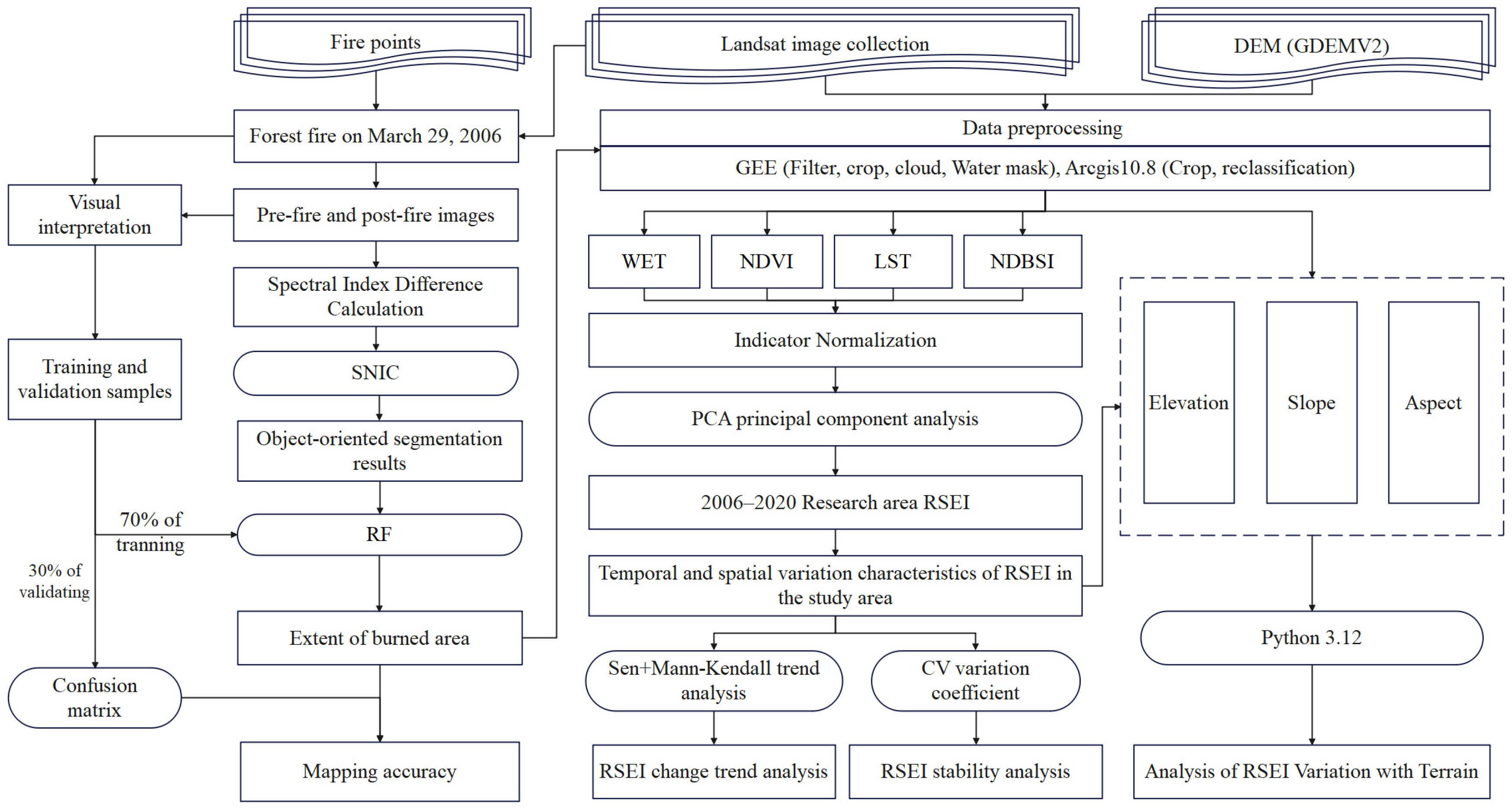
2.3.1. Research Technical Workflow

The research technical workflow of this study is shown in Figure 2.

2.3.2. Burned Area Extraction

This study generated Landsat difference images for seven spectral indices—NDVI [45], normalized burn ratio (NBR) [46], EVI [47], normalized difference moisture index (NDMI) [45], normalized difference water index (NDWI) [48], soil-adjusted vegetation index (SAVI) [49], and bare soil index (BSI) [50]—on the GEE platform. The images were then segmented using the Simple Non-Iterative Clustering (SNIC) algorithm [51], and the segmentation results were input into a random forest (RF) model to extract the burned area extent. In this study, 122 forest fire sample points and 120 non-forest fire sample points were labeled through visual interpretation and split into training and validation datasets with a 7:3 ratio. RF uses decision trees using randomly sampled data subsets and features and combines their predictions through averaging or voting. This reduces overfitting and improves the model’s generalization ability [52]. The overall accuracy (OA, Equation (1)), user accuracy (UA, Equation (2)), producer accuracy (PA, Equation (3)), and F1-score (Equation (4)) were calculated using a confusion matrix to assess the model’s classification performance [53].

$$OA={\displaystyle \frac{TP+TN}{TP+FN+FP+TN}}$$

(1)

$$UA={\displaystyle \frac{TP}{TP+FP}}$$

(2)

$$PA={\displaystyle \frac{TP}{TP+FN}}$$

(3)

$$F1\text{-}Score=2\ast {\displaystyle \frac{Precision\ast Recall}{Precision+Recall}}$$

(4)

where TP, FP, TN, and FN represent true positive, false positive, true negative, and false negative, respectively.

2.3.3. RSEI Construction

In our study, the RSEI was computed on an annual basis from 2005 to 2020 with the help of the GEE platform (Equation (5)). The RSEI is formulated by integrating four key indicators: greenness, wetness, dryness, and heat [18,26] (

Table 2. The calculation formulas and explanations for NDVI, WET, LST, and NDSI.

Indicators	Index	Formula	Explanation
Greenness	NDVI	$NDVI={\displaystyle \frac{{\rho }_{NIR}-{\rho }_{Red}}{{\rho }_{NIR}+{\rho }_{Red}}}$	${\rho }_{NIR}$ represents the near-infrared band, while ${\rho }_{Red}$ represents the red band [26].
Wetness	WET	$WET={\beta }_1{\rho }_{Blue}+{\beta }_2{\rho }_{Green}+{\beta }_3{\rho }_{Red}+{\beta }_4{\rho }_{NIR}+{\beta }_5{\rho }_{SWIR1}+{\beta }_6{\rho }_{SWIR2}$	${\rho }_{Blue}, {\rho }_{Green}, {\rho }_{Red}, {\rho }_{NIR}, {\rho }_{SWIR1}, {\rho }_{SWIR2}$ represent the bands of Landsat 5, 7, and 8, respectively [26,54].
Heat	LST	$LST=\gamma \left[{\displaystyle \frac{1}{\epsilon }}\times \left({\psi }_1\times L_{sen}+{\psi }_2\right)+{\psi }_3\right]+\delta$	The calculation of parameters refers to [55,56,57].
Dryness	NDBSI	$NDBSI={\displaystyle \frac{IBI+SI}{2}}$ $IBI={\displaystyle \frac{\frac{2{\rho }_{SWIR1}}{{\rho }_{SWIR1}+{\rho }_{NIR}}-\left[\frac{{\rho }_{NIR}}{{\rho }_{NIR}+{\rho }_{Red}}+\frac{{\rho }_{Green}}{{\rho }_{Green}+{\rho }_{SWIR1}}\right]}{\frac{2{\rho }_{SWIR1}}{{\rho }_{SWIR1}+{\rho }_{NIR}}+\left[\frac{{\rho }_{NIR}}{{\rho }_{NIR}+{\rho }_{Red}}+\frac{{\rho }_{Green}}{{\rho }_{Green}+{\rho }_{SWIR1}}\right]}}$ $SI={\displaystyle \frac{\left({\rho }_{SWIR1}+{\rho }_{Red}\right)-\left({\rho }_{NIR}+{\rho }_{Blue}\right)}{\left({\rho }_{SWIR1}+{\rho }_{Red}\right)+\left({\rho }_{NIR}+{\rho }_{Blue}\right)}}$	SI represents the Soil Index, and IBI represents the Building Index [7,26].
/	mNDWI	$mNDWI={\displaystyle \frac{{\rho }_{Green}-{\rho }_{SWIR1}}{{\rho }_{Green}+{\rho }_{SWIR1}}}$	${\rho }_{Green}$ and ${\rho }_{SWIR1}$ represent the green and shortwave infrared 1 bands, respectively [58].

). Additionally, water body information has a significant impact on the wetness indicator. Therefore, prior to the RSEI calculation, water bodies were masked using the modified Normalized Difference Water Index (mNDWI).

$$RSEI=f\left(Greenness, Wetness, Heat, Dryness\right)$$

(5)

The values of the four metrics were mapped to the range [0, 1] through normalization (Equation (6)).

$$NI={\displaystyle \frac{X_i-X_{min}}{X_{max}-X_{min}}}$$

(6)

where NI represents the normalized indicator; $X_i$ denotes the indicator’s original value; and $X_{min}$ and $X_{max}$ denote the minimum and maximum values of the original indicator, respectively.

The RSEI was constructed using PCA [59], with the first principal component (PC1) serving as the starting value of RSEI, denoted as $RSE{I}_0$ (Equation (7)). If the contribution rate of PC1 is significantly greater than that of other principal components, it indicates that PC1 encompasses most of the information.

$$RSE{I}_0=1-PC1\left[f\left(NDVI, WET, NDBSI, LST\right)\right]$$

(7)

where PC1 represents the first principal component derived from the four indices: NDVI, WET, NDSI, and LST.

The normalized $RSE{I}_0$ was used as the final RSEI, with values closer to 1 indicate higher EQ. The RSEI is categorized into five levels at 0.2 intervals [7,18,26].

2.3.4. Theil–Sen Estimator and MK Trend Test

Trends in RSEI in the burned area between 2006 and 2020 were analyzed by Theil–Sen slope estimation and evaluated for statistical significance using the MK trend test. The combination of the Theil–Sen slope method and the MK trend test can effectively reduce the impact of outliers on the results [60].

The Theil–Sen estimator calculates the slope between all paired points through simple linear regression and fits the linear trend using the median of these slopes. The Theil–Sen slope test calculates the slope for all data pairs in the time series and uses the median slope (Equation (8)) as the representative of the overall trend [61].

$$\beta =Median\left({\displaystyle \frac{RSE{I}_j-RSE{I}_i}{j-i}}\right), {\forall }_j>i$$

(8)

where $Median\left( \right)$ represents the median value, and $RSE{I}_j$ and $RSE{I}_i$ correspond to the RSEI values for the years j and i in the time series. A positive $\beta$ value indicates an upward trend, while a negative $\beta$ value indicates a downward trend.

The MK trend test is employed to assess the significance of trends in long-time series data [39]. The test statistic S is calculated (Equation (9)) [62]:

$$S={\displaystyle \sum _{i=1}^{n-1}}{\displaystyle \sum _{j=i+1}^n}sgn\left(RSE{I}_j-RSE{I}_i\right)$$

(9)

where $sgn\left( \right)$ represents the sign function, and the formula is given in Equation (10).

$$sgn\left(NDV{I}_j-NDV{I}_i\right)=\left\{\begin{array}{c}1,RSE{I}_j-RSE{I}_i>0\\ 0,RSE{I}_j-RSE{I}_i=0\\ -1,RSE{I}_j-RSE{I}_i<0\end{array}\right.$$

(10)

The choice of test statistic for significance testing varies depending on the length n of the time series; for cases where n < 8, S is applied directly for a two-sided trend test. When n ≥ 8, the test statistic S can be approximated by a standard normal distribution, and the Z statistic is employed for trend testing [39,63], with the Z value calculated by (Equation (11)):

$$Z=\left\{\begin{array}{c}{\displaystyle \frac{S-1}{\sqrt{VAR\left(S\right)}}}, S>0\\ 0, S=0\\ {\displaystyle \frac{S+1}{\sqrt{VAR\left(S\right)}}},S<0\end{array}\right.$$

(11)

where $VAR\left(S\right)$ is calculated by Equation (12):

$$VAR\left(S\right)={\displaystyle \frac{n\left(n+1\right)\left(2n+5\right)}{18}}$$

(12)

The time series analyzed in this study spans 15 years (from 2006 to 2020), so the test statistic Z is employed for trend analysis. The specific criteria for determining trend significance are detailed in

Table 3. Mann–Kendall test trend categories.

β	Z	Trend Features
β > 0	2.58 < Z	Extremely significant increase
	1.96 < Z ≤ 2.58	Significant increase
	1.65 < Z ≤ 1.96	Slight increase
	Z ≤ 1.65	Insignificant increase
β = 0	Z	Unchanged
β < 0	Z ≤ 1.65	Insignificant decrease
	1.65 < Z ≤ 1.96	Slight decrease
	1.96 < Z ≤ 2.58	Significant decrease
	2.58 < Z	Extremely significant decrease

.

2.3.5. Stability Analysis

The CV is a statistical parameter used to measure the dispersion of a variable (Equation (13)) and can effectively reflect the fluctuation of time series data [40]. This study focuses on the period from 2006 to 2020 for analysis. The CV of RSEI is calculated pixel by pixel, and the results are grouped into five categories—low, relatively low, moderate, relatively high, and high fluctuation—using the natural breaks classification method [64]. A higher CV value indicates a greater dispersion in the distribution of RSEI values, indicating greater intensity of ecosystem disturbance and lower environmental stability; conversely, the opposite is true.

$$CV={\displaystyle \frac{\sigma }{\overline{RSEI}}}={\displaystyle \frac{\sqrt{\frac{1}{n}{\displaystyle {\sum }_{i=1}^n}{\left(RSE{I}_i-\overline{RSEI}\right)}^2}}{\overline{RSEI}}}$$

(13)

where, $\sigma$ represents the standard deviation, and $\overline{RSEI}$ denotes the mean RSEI over n years.

2.3.6. Terrain Analysis

To investigate the impact of topographic factors like elevation, slope, and aspect on post-fire EQ, the average RSEI values for each factor were calculated. The elevation was divided into four intervals: 1800–2000 m, 2000–2200 m, 2200–2400 m, and 2400–2600 m. According to the national standard technical regulations for inventory for forest management planning and design (GB/T 26424-2010) [65], the slope is classified into flat slope (0–5°), gentle ascent (5–15°), slant slopes (15–25°), steep slopes (25–35°), abrupt slopes (35–45°), and dangerous slopes (>45°). Aspect values are categorized into nine divisions, encompassing the four cardinal directions (north, east, south, west), four intercardinal directions (northeast, southeast, southwest, northwest), and flat.

3. Results

3.1. Extraction of Burned Area Extent

This study extracted the boundary of the burned area from the forest fire in Anning City on 29 March 2006 (Figure 1c). The extraction results show that the overall accuracy and F1-score of the burned area exceed 95%, with an extracted area of 1513.26 hm².

3.2. Spatiotemporal Dynamics Analysis of RSEI

3.2.1. RSEI Feature Extraction Using PCA

Based on the PCA results of RSEI from May to October for each year from 2005 to 2020 within the burned area boundary (

Table 4. The PC1 analysis results.

Year	PC1 Eigenvector				Contribution Rate (%)
	WET	NDVI	LST	NDBSI
2005	0.26	0.49	−0.47	−0.69	67.51
2006	0.38	0.47	−0.46	−0.64	65.52
2007	0.38	0.48	−0.49	−0.61	66.61
2008	0.13	0.61	−0.35	−0.70	55.68
2009	0.31	0.50	−0.52	−0.62	63.17
2010	0.35	0.58	−0.44	−0.59	64.28
2011	0.27	0.53	−0.53	−0.60	60.88
2012	0.37	0.55	−0.50	−0.56	68.07
2013	0.33	0.48	−0.55	−0.60	64.66
2014	0.35	0.56	−0.53	−0.53	69.34
2015	0.29	0.52	−0.51	−0.63	66.55
2016	0.39	0.29	−0.45	−0.75	57.36
2017	0.47	0.39	−0.60	−0.52	63.36
2018	0.50	0.38	−0.58	−0.51	62.78
2019	0.53	0.42	−0.62	−0.41	63.79
2020	0.50	0.42	−0.66	−0.37	68.07
Mean	0.36	0.48	−0.52	−0.58	64.23

), the contribution rate of variance explained by PC1 exceeds 64.23%. This suggests that PC1 effectively encapsulates the core information derived from the four indicators, providing a reliable representation of the study area’s ecological status. In PC1, both NDVI and WET show positive loadings, suggesting that these two indicators contribute positively to the ecological environment. Conversely, LST and NDBSI have negative loadings, suggesting that these two indicators collectively have a negative effect on the ecological environment. The eigenvector analysis reveals that, among the four indicators, NDBSI has the largest absolute loading value, which suggests that aridity significantly contributes to shaping the RSEI within the research region.

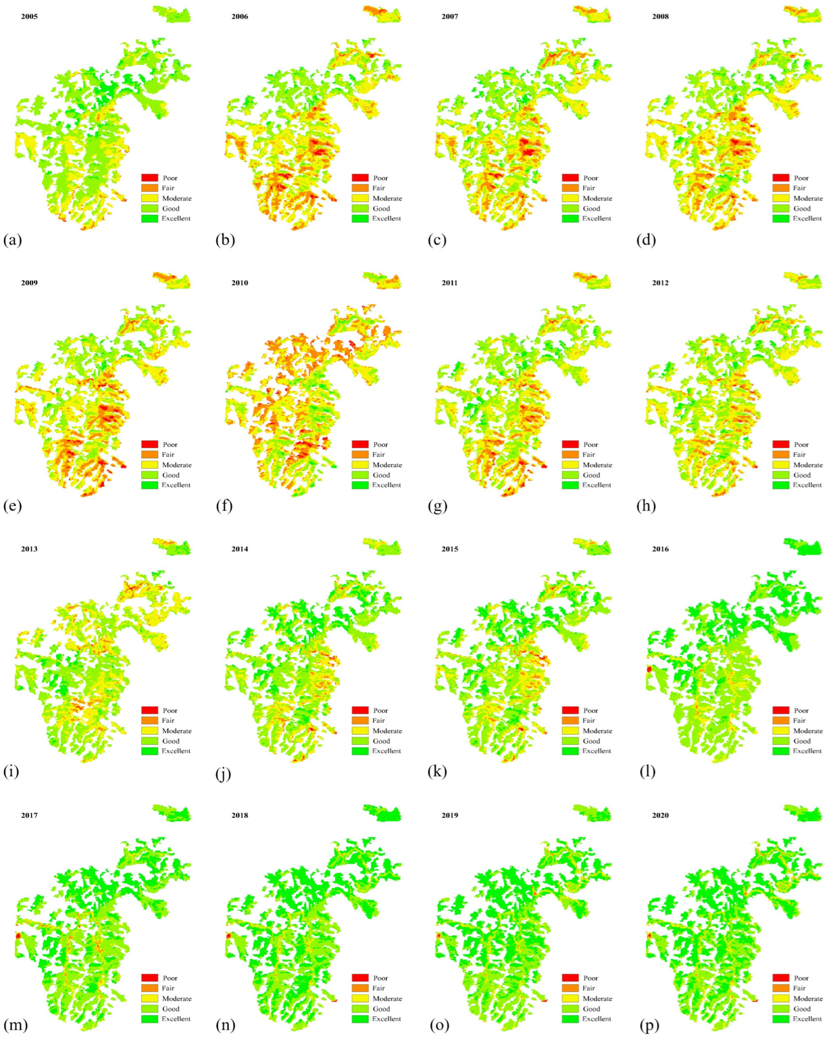
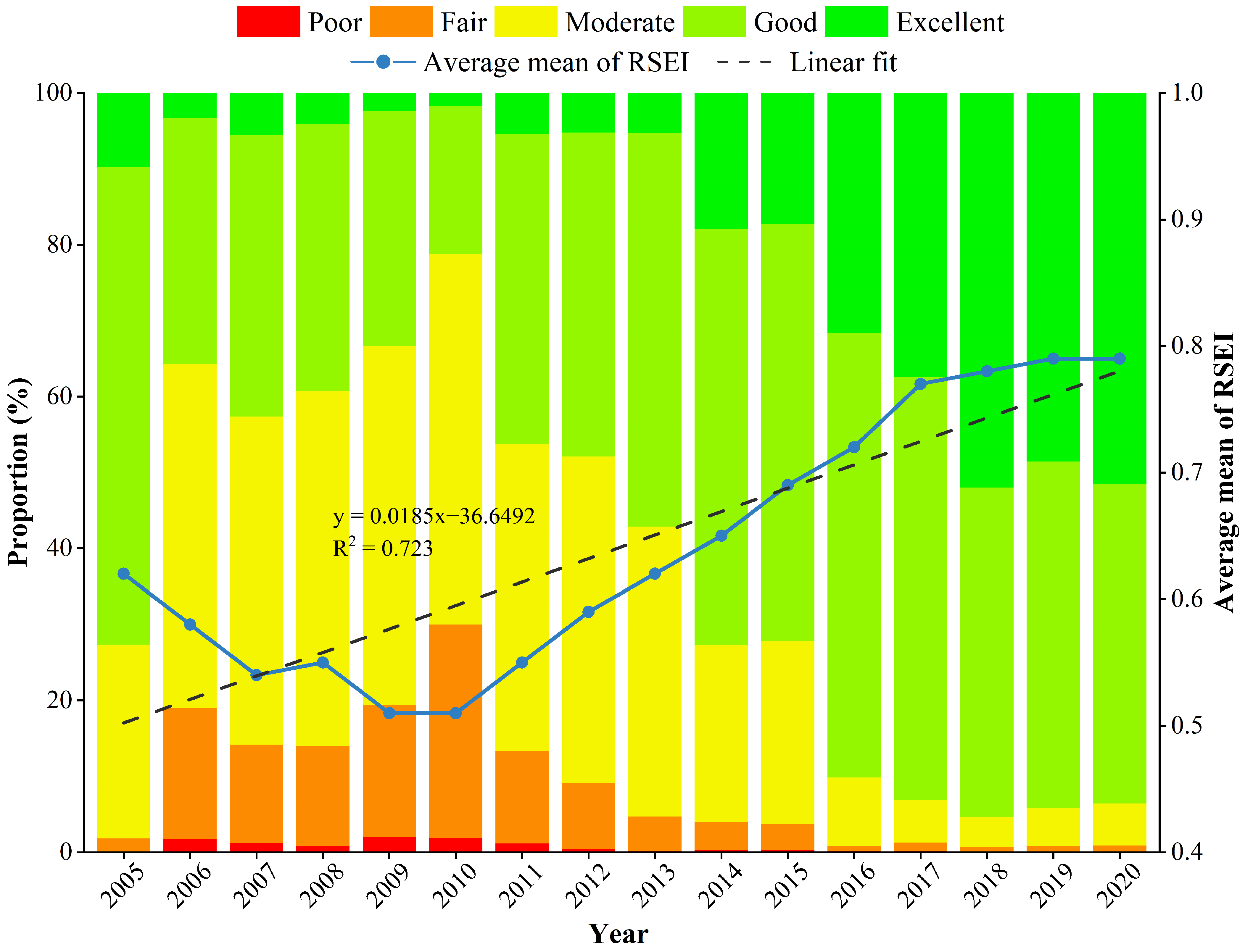
3.2.2. Temporal and Spatial Analysis of RSEI

The spatial distribution of RSEI in the study area from 2005 to 2020 (Figure 3) shows significant variations in EQ across different years, undergoing a process of decline (2006–2010), gradual increase (2011–2016), and eventual stabilization (2017–2020). Following the forest fire in 2006, the EQ within the burned area significantly declined, with the most pronounced degradation observed between 2007 and 2010, where regions of low (poor and fair) and moderate ecological grades predominated. Since 2011, the EQ gradually recovered, with a notable reduction in low-grade areas and a significant expansion of moderate and high-grade regions, leading to a progressive improvement in EQ. After 2016, most of the area within the burned area reached ‘good’ and ‘excellent’ grades, and the spatial distribution stabilized. The results indicate that the long-term impact of the fire on the EQ has been effectively alleviated, and the ecosystem in the study area has demonstrated strong self-restoration capabilities.

Based on the distribution percentage and trend of the average RSEI values for each grade over 16 years in the study area (Figure 4), the RSEI values showed an overall trend of “decline initially-fluctuating increase-stabilization” after the fire. After the forest fire in 2006, the RSEI value dropped significantly, with the percentage of areas classified as ’good’ and ’excellent’ falling sharply from 72.65% in 2005 to 35.73%. By 2010, the average RSEI value dropped to its lowest point (0.51), indicating that the fire caused significant damage to EQ. From 2011 to 2013, the RSEI value gradually recovered, though the recovery was relatively slow. After 2014, the recovery accelerated significantly, and the RSEI value surpassed the pre-fire level (0.60). The linear fitting results reveal that the average annual change rate of RSEI is 0.0185 a⁻¹, with a fitting degree of 0.723, indicating a significant recovery trend in the post-fire EQ of the forest. Since 2017, the average RSEI value has stabilized above 0.75, reflecting that the EQ within the burned area has largely returned to a ’good’ condition. From 2005 to 2020, the RSEI classification statistics indicate that the proportion of areas rated as ’good’ and ’excellent’ varied each year, rising from 35.73% in 2006 to 93.57% in 2020, with a growth rate of 161.88%. Overall, the fire caused considerable short-term damage to the ecological system, but the region demonstrated strong natural ecological recovery capabilities, and the forest EQ was restored and maintained at a stable level post-fire.

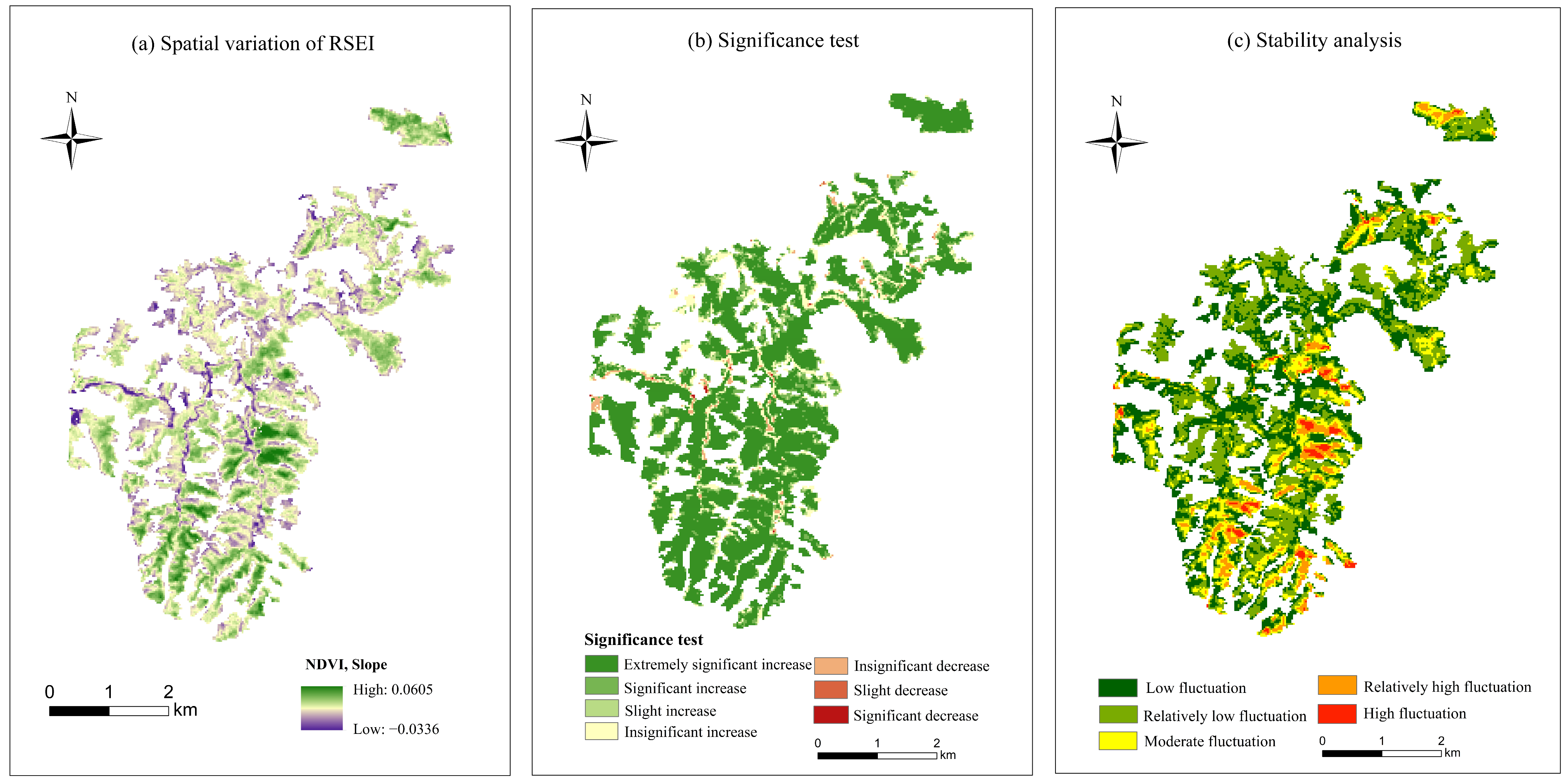
3.2.3. RSEI Trend Change Analysis

Based on the trend of RSEI mean values during the vegetation growing season in the burned area from 2006 to 2020 and its significance analysis (Figure 5a,b and

Table 5. RSEI changes significance statistics.

Change Trend Type	Area (hm2)	Proportion (%)
Significant decrease	1.12	0.07
Slight decrease	0.56	0.04
Insignificant decrease	25.53	1.69
Insignificant increase	150.14	9.92
Slight increase	59.99	3.96
Significant increase	215.79	14.26
Extremely significant increase	1060.14	70.06

), the RSEI change trends are classified into seven categories: extremely significant increase, a significant increase, slight increase, insignificant increase, insignificant decrease, slight decrease, and significant decrease. From Figure 5a,b, it is evident that the RSEI in the study area exhibits an overall trend of extremely significant increase, with a change slope range from −0.0336 to 0.0605 a⁻¹. The portion of the burned area that experienced an extremely significant increase is 70.06%, while 14.26% of the area showed a significant increase. The areas exhibiting a decreasing trend make up only 1.80%, primarily distributed around the central fire barrier zone. Among them, the significant decrease was 0.07%, the slight decrease was 0.04%, and the insignificant decrease was 1.69%. Additionally,

Table 6. RSEI stability classification statistics.

CV	Fluctuation Classes	Area (hm2)	Proportion (%)
<0.188	Low	543.46	35.91
0.188–0.241	Relatively low	629.63	41.61
0.241–0.323	Moderate	219.15	14.48
0.323–0.472	Relatively high	96.78	6.40
>0.472	High	24.24	1.60

shows that between 2006 and 2020, the RSEI in the burned area exhibited an increasing trend, covering 1486.07 hm², which represents 98.20% of the total burned area. In summary, the EQ in the study area has seen substantial recovery post-fire, with most regions showing significant or highly significant growth trends, while only a few localized areas have experienced a decrease.

3.2.4. RSEI Stability Analysis

To explore the post-fire fluctuations in EQ within the study area, the variability was divided into five categories according to the RSEI CV (Table 6). Additionally, a map depicting the spatial distribution of RSEI variability from 2006 to 2020 was produced (Figure 5c). The overall CV of RSEI is 0.16, indicating that the EQ of the study area has generally stabilized and recovered post-fire, with minor fluctuations; however, some localized areas still show variations. Figure 5c illustrates a clear spatial variation in the RSEI CV, which shows significant heterogeneity. Table 4 shows that the proportion of low and relatively low fluctuation areas accounted for 77.52% (1173.09 hm²), indicating that most of the EQ restoration in the burned area has a high degree of stability. In contrast, areas with moderate, relatively high, and high fluctuation account for only 22.48%, indicating that the recovery process in a small portion of the area shows some instability.

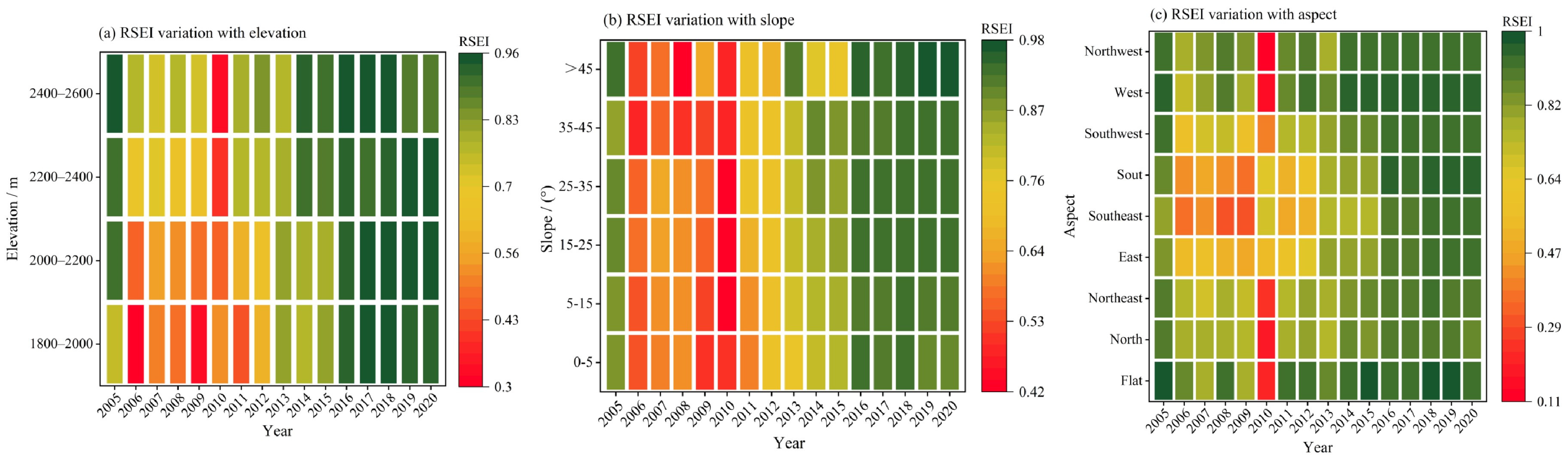
3.2.5. Terrain Effects on RSEI

Figure 6 shows the terrain effects on EQ after the fire at different elevations, slopes, and aspects. Figure 6a shows that the fire had the most significant ecological impact in the low elevation range of 1800–2200 m, while the higher elevations between 2400–2600 m experienced comparatively less damage. RSEI values recovered progressively over time at all elevation intervals, but recovery was slower at lower elevations and faster at higher elevations. As seen in Figure 6b, the fire caused more severe damage to areas with slopes greater than 35°. During the recovery process, areas with gentler slopes recovered more quickly, while areas with steeper slopes recovered more slowly. Figure 6c shows the recovery situation in different aspects. It can be observed that southeast < south < east < southwest < west < northeast < north < northwest < flat, indicating that sun-facing slopes (such as southeast and south slopes) experience more severe ecological damage due to higher temperatures and more intense burning. In contrast, shaded slopes (such as northwest and north slopes) experience less ecological damage and recover more quickly. Overall, the ecological impact of the fire is more significant in low-altitude, steep, and sun-facing slope areas, with slower recovery, while recovery is faster in high-altitude, gentler, and shaded slope areas.

4. Discussion

4.1. First Revealing the Temporal and Spatial Variation Patterns of Forest EQ Post-Fire in Complex Plateau Mountain Areas

This study is the first attempt to explore the temporal and spatial patterns of long-term dynamic recovery of forest EQ in complex plateau mountain areas post-fire. As shown in Figure 4 and Figure 5, the overall trend of forest EQ after the fire presents a pattern of “decline initially-fluctuating increase-stabilization”, which indicates that fire has a significant impact on EQ. Specifically, significant changes in spectral index characteristics due to massive loss of vegetation, destruction of chlorophyll, increased soil exposure, and changes in surface moisture content have led to a dramatic decline in forest EQ [66]. With the reduction of anthropogenic disturbances and the gradual restoration of vegetation cover, the EQ begins to improve. However, there are limits to the ability of ecosystems to repair themselves, while short-term climatic extremes (e.g., extreme drought) may have an impact on vegetation recovery, leading to fluctuating increases in the EQ of forests during the recovery process [67,68]. Finally, with the increase in vegetation cover, the enhancement of soil and water conservation capacity, and the improvement of internal ecosystem processes, EQ tends to stabilize, and the forest ecosystem gradually restores to a new equilibrium state. Currently, most studies primarily focus on using time series of a single spectral index to assess vegetation recovery post-fire [16,23]. However, this approach is limited in its ability to fully reflect the complex impacts of fire on ecosystem quality. In comparison, RSEI, through the coupling of four indicators—greenness, wetness, heat, and dryness [26]—not only effectively reflects the reduction in greenness and wetness due to the fire, but also indicates the extent of soil exposure and changes in heat. This enables a more thorough depiction of the intricate and multidimensional dynamic changes during the post-fire ecological recovery process. This study is important for understanding the mechanisms of post-fire forest EQ restoration in the complex mountainous areas of the plateau. By introducing the RSEI composite index, the limitations of traditional single spectral indices have been overcome, enabling a more comprehensive and precise revelation of the multidimensional changes in the post-fire ecological environment. The findings of this study offer a scientific foundation for monitoring and managing ecological restoration, as well as assisting in the development of policies for ecological restoration, wildfire risk evaluation, and sustainable forest management.

4.2. RSEI Is Applicable for EQ Assessment at the Scale of Burned Areas in Complex Mountainous Plateaus

This study, based on Landsat imagery, constructed the extent of the burn scar in Anning City, Yunnan Province, on 29 March 2006 (1513.26 hm²). The RSEI time series from 2005 to 2020 revealed that the post-fire forest EQ exhibited a trend of “decline initially-fluctuating increase-stabilization”, showing overall improvement year by year. RSEI effectively integrates the key aspects of four indicators—greenness, wetness, heat, and dryness—allowing for a precise reflection of the regional ecosystem’s quality. Among these, greenness and wetness contribute positively to EQ, while heat and dryness exert negative impacts on EQ. This result is consistent with studies in non-mountainous plain areas [10,11].

The accuracy of RSEI in assessing the post-fire forest EQ recovery patterns in plateau mountainous regions relies on precise burned area mapping. The study area is in a plateau mountainous region characterized by significant terrain undulations, large altitude variations, distinct vertical climate differentiation, diverse vegetation types, and strong spatial heterogeneity in the ecological environment. These factors contribute to a more complex and uncertain process of post-fire forest EQ recovery. To address the complex factors in plateau mountainous regions, this study used Landsat difference images of seven vegetation indices—NDVI, NBR, EVI, NDMI, NDWI, SAVI, and BSI—combined with the SNIC superpixel segmentation algorithm and the RF classifier to achieve precise extraction of the burn area extent. The SNIC algorithm performs spatial segmentation on the image, ensuring that superpixels maintain similarity in both color and spatial location, thereby preserving boundary details while reducing classification noise and minimizing discrete pixels and the “salt-and-pepper” phenomenon [69]. Compared to a single vegetation index, the integration of multiple indices can provide more comprehensive surface information, enhance the model’s ability to identify land cover features, and thus improve classification accuracy [70,71]. The RF classifier, as an ensemble learning method, possesses strong robustness, effectively handles high-dimensional data, and reduces the risk of overfitting [72]. This study enhances the applicability of RSEI in plateau mountainous regions by accurately extracting the burned area extent, allowing it to more precisely reflect the dynamic changes in post-fire forest EQ.

Currently, the application of RSEI time series in large-scale regional EQ assessments has been widely validated [4,5,8]. These studies have revealed patterns of regional EQ changes and demonstrated the effectiveness of RSEI in large-scale ecological assessments. In contrast, this study focuses on the post-fire forest EQ recovery process at a small scale, further validating the applicability of RSEI in small-scale EQ assessments. This study provides new perspectives and methodological support for post-fire forest EQ recovery in complex plateau mountainous environments.

4.3. Post-Fire Forest EQ Recovery Exhibits Significant Topographic Effects

Different topographic factors have significant effects on post-fire vegetation recovery [73], which is an important aspect of EQ restoration. This study reveals the significant influence of topography on post-fire forest EQ recovery by analyzing changes in RSEI from 2005 to 2020 across different elevations, slopes, and aspects (Figure 6). The study found that fires have a greater ecological impact on low-altitude areas, steep slopes, and sun-facing slopes, with slower recovery rates, while high-altitude areas, gentle slopes, and shaded slopes recover more quickly. The possible reason for this result is that high-altitude areas have lower temperatures and thinner oxygen, which hinder fire spread, making them less affected. As a result, the RSEI values remain stable and recover more quickly. In areas with gentle slopes, the spread of fires is slower, allowing more time for firefighting and resulting in a smaller affected area and a smaller decline in RSEI values. Shaded slopes, due to less sunlight, lower temperatures, and higher humidity, experience slower fire spread, lighter ecological damage, and a smaller decline in RSEI values. The sun-facing slopes (southeast and south slopes) are exposed to direct sunlight for extended periods, resulting in higher surface temperatures, which promote evapotranspiration and lead to a reduction in air humidity. In addition, sunny slopes are dominated by drought-tolerant vegetation (e.g., shrubs and herbs), whose lower moisture content makes them more flammable. The buildup of flammable matter, such as dried leaves and branches, further elevates the risk of fire [74]. After the fires, the ecological recovery of the sunny slopes was slow, mainly affected by high temperatures and increased water evaporation, resulting in persistently low soil moisture content. Additionally, the fire destroyed the vegetation structure, causing the soil to lose the protective cover of vegetation, which accelerated water loss and further restricted the natural recovery capacity of the vegetation, leading to a slower process of EQ restoration [75]. It is recommended that relevant departments comprehensively consider elevation, slope, and aspect factors to conduct fire risk assessments, strengthen routine inspections and monitoring, and reasonably plan infrastructure such as firebreaks and fire access roads to enhance fire prevention and control capabilities.

4.4. Uncertainty Analysis

Although this study has validated the effectiveness of RSEI in assessing the spatiotemporal changes of post-fire forest EQ, some limitations and uncertainties still exist. Firstly, the RSEI evaluation method mainly emphasizes four factors: greenness, wetness, heat, and dryness. However, the impact of fires on forest ecosystems is complex and diverse. Future research could incorporate more factors and develop new indicators to systematically evaluate the changes and recovery processes of post-fire forest EQ. Secondly, the time series data for this study were obtained from Landsat 5 TM, Landsat 7 ETM+, and Landsat 8 OLI sensors, which have inherent spectral differences that cannot be fully removed. To ensure data consistency, future research could prioritize using data from a single sensor to reduce uncertainties caused by spectral variations. Third, to address the issue of image gaps caused by cloud shadows, this study utilized images from the two months preceding and following the vegetation growing season for gap-filling, thereby maintaining temporal continuity. However, the temporal differences between images and ecological changes were not considered, which could impact the accuracy of the gap-filling data. Future studies might investigate more advanced gap-filling techniques, such as machine learning-based time-series interpolation or the integration of remote sensing data from multiple sources, to improve the precision and dependability of the findings. Finally, when analyzing the changes in RSEI across different elevations, slopes, and aspects, we observed that the average RSEI value in 2010 was anomalously low, even lower than that of 2006, the year the fire occurred (Figure 6). The literature indicates that during the period from 2009 to 2010, Southwest China (including the five provinces, municipalities, and autonomous regions of Yunnan, Guangxi, Guizhou, Sichuan, and Chongqing) experienced extreme drought conditions [76,77]. Drought years are generally linked to a reduction in soil moisture, which limits plant growth, resulting in less vegetation cover and lower NDVI values, thus influencing the RSEI calculation. Particularly in extreme drought years, severe soil moisture deficiency and reduced air humidity limit plant growth, subsequently decreasing ecosystem productivity and leading to a decline in RSEI values. However, RSEI primarily assesses EQ using remote sensing data (such as NDVI, LST, WET, and NDBSI). These remote sensing data provide long-term and spatially extensive information on ecological changes, which may not fully capture short-term or localized variations in EQ. Therefore, future research should incorporate multi-source data fusion and include additional variables, such as soil properties (e.g., soil moisture, permeability), species composition (e.g., species diversity and resilience), and meteorological data (e.g., precipitation, temperature, evapotranspiration), to enhance the accuracy of post-fire forest EQ restoration assessments.

5. Conclusions

In this study, Landsat series data and difference images from multiple vegetation indices were processed using the GEE platform, segmented by SNIC, and then input into the RF model to extract the extent of the burned area. A 2005–2020 RSEI time series was constructed, and the recovery of post-fire forest EQ was evaluated using the Theil–Sen estimator, MK trend test, stability analysis, and topographic factors. The main research conclusions are as follows: (1) Under conditions of comparable mapping accuracy to non-mountainous plains, RSEI can also be applied to forest EQ assessment in complex plateau mountainous regions. (2) The post-fire forest EQ in plateau mountainous areas can return to pre-fire conditions within 10 years, with the recovery process exhibiting a three-stage pattern: “decline initially-fluctuating increase-stabilization”. (3) Between 2006 and 2020, the forest EQ in the study region demonstrated a spatial pattern of increasing high-quality areas; temporally, it exhibited a consistent annual increase in overall EQ, with good overall stability in the recovery process. (4) The EQ of forests in low-altitude areas, on steep slopes, and sun-facing slopes changed significantly after the fire compared to the pre-fire period, with a slower rate of recovery and notable topographic effects.

References

1. Ballantyne, A.; Smith, W.; Anderegg, W.; Kauppi, P.; Sarmiento, J.; Tans, P.; Shevliakova, E.; Pan, Y.; Poulter, B.; Anav, A.; et al. Accelerating Net Terrestrial Carbon Uptake during the Warming Hiatus Due to Reduced Respiration. Nat. Clim. Change 2017, 7, 148–152. [Google Scholar] [CrossRef]
2. Guo, F.; Su, Z.; Tigabu, M.; Yang, X.; Lin, F.; Liang, H.; Wang, G. Spatial Modelling of Fire Drivers in Urban-Forest Ecosystems in China. Forests 2017, 8, 180. [Google Scholar] [CrossRef]
3. Loydi, A.; Funk, F.A.; García, A. Vegetation Recovery after Fire in Mountain Grasslands of Argentina. J. Mt. Sci. 2020, 17, 373–383. [Google Scholar] [CrossRef]
4. Yang, X.; Meng, F.; Fu, P.; Zhang, Y.; Liu, Y. Spatiotemporal Change and Driving Factors of the Eco-Environment Quality in the Yangtze River Basin from 2001 to 2019. Ecol. Indic. 2021, 131, 108214. [Google Scholar] [CrossRef]
5. Yuan, B.; Fu, L.; Zou, Y.; Zhang, S.; Chen, X.; Li, F.; Deng, Z.; Xie, Y. Spatiotemporal Change Detection of Ecological Quality and the Associated Affecting Factors in Dongting Lake Basin, Based on RSEI. J. Clean. Prod. 2021, 302, 126995. [Google Scholar] [CrossRef]
6. An, M.; Xie, P.; He, W.; Wang, B.; Huang, J.; Khanal, R. Spatiotemporal Change of Ecologic Environment Quality and Human Interaction Factors in Three Gorges Ecologic Economic Corridor, Based on RSEI. Ecol. Indic. 2022, 141, 109090. [Google Scholar] [CrossRef]
7. Hu, X.; Xu, H. A New Remote Sensing Index for Assessing the Spatial Heterogeneity in Urban Ecological Quality: A Case from Fuzhou City, China. Ecol. Indic. 2018, 89, 11–21. [Google Scholar] [CrossRef]
8. Lv, Y.; Xiu, L.; Yao, X.; Yu, Z.; Huang, X. Spatiotemporal Evolution and Driving Factors Analysis of the Eco-Quality in the Lanxi Urban Agglomeration. Ecol. Indic. 2023, 156, 111114. [Google Scholar] [CrossRef]
9. Miao, W.; Chen, Y.; Kou, W.; Lai, H.; Sazal, A.; Wang, J.; Li, Y.; Hu, J.; Wu, Y.; Zhao, T. The HANTS-Fitted RSEI Constructed in the Vegetation Growing Season Reveals the Spatiotemporal Patterns of Ecological Quality. Sci. Rep. 2024, 14, 14686. [Google Scholar] [CrossRef]
10. Liu, C.; Yang, M.; Hou, Y.; Zhao, Y.; Xue, X. Spatiotemporal Evolution of Island Ecological Quality under Different Urban Densities: A Comparative Analysis of Xiamen and Kinmen Islands, Southeast China. Ecol. Indic. 2021, 124, 107438. [Google Scholar] [CrossRef]
11. Wang, X.; Nian, Y.; Wang, H.; Chen, J.; Li, K.; Hu, T.; Li, Z. Monitoring of Ecological Environment Changes in Open-Pit Mines on the Loess Plateau from 1990 to 2023 Based on RSEI. Ecol. Indic. 2025, 170, 113064. [Google Scholar] [CrossRef]
12. Qureshi, S.; Alavipanah, S.K.; Konyushkova, M.; Mijani, N.; Fathololomi, S.; Firozjaei, M.K.; Homaee, M.; Hamzeh, S.; Kakroodi, A.A. A Remotely Sensed Assessment of Surface Ecological Change over the Gomishan Wetland, Iran. Remote Sens. 2020, 12, 2989. [Google Scholar] [CrossRef]
13. Crausbay, S.D.; Higuera, P.E.; Sprugel, D.G.; Brubaker, L.B. Fire Catalyzed Rapid Ecological Change in Lowland Coniferous Forests of the Pacific Northwest over the Past 14,000 Years. Ecology 2017, 98, 2356–2369. [Google Scholar] [CrossRef]
14. Qiu, J.; Wang, H.; Shen, W.; Zhang, Y.; Su, H.; Li, M. Quantifying Forest Fire and Post-Fire Vegetation Recovery in the Daxin’anling Area of Northeastern China Using Landsat Time-Series Data and Machine Learning. Remote Sens. 2021, 13, 792. [Google Scholar] [CrossRef]
15. Jiang, B.; Chen, W.; Wu, Y.; Gao, Z. Monitoring Vegetation Restoration after Wildfires in Typical Boreal Forests Based on Multi-Source Remote Sensing Data. In Proceedings of the Igarss 2024—2024 IEEE International Geoscience and Remote Sensing Symposium, Athens, Greece, 7–12 July 2024; pp. 581–584. [Google Scholar]
16. Viana-Soto, A.; Aguado, I.; Martínez, S. Assessment of Post-Fire Vegetation Recovery Using Fire Severity and Geographical Data in the Mediterranean Region (Spain). Environments 2017, 4, 90. [Google Scholar] [CrossRef]
17. Waring, R.H.; Coops, N.C.; Fan, W.; Nightingale, J.M. MODIS Enhanced Vegetation Index Predicts Tree Species Richness across Forested Ecoregions in the Contiguous U.S.A. Remote Sens. Environ. 2006, 103, 218–226. [Google Scholar] [CrossRef]
18. Hanqiu, X. A Remote Sensing Urban Ecological Index and Its Application. Acta Ecol. Sin. 2014, 33, 7853–7862. [Google Scholar] [CrossRef]
19. Zhang, S.; Bai, M.; Wang, X.; Peng, X.; Chen, A.; Peng, P. Remote Sensing Technology for Rapid Extraction of Burned Areas and Ecosystem Environmental Assessment. PeerJ 2023, 11, e14557. [Google Scholar] [CrossRef]
20. Wang, R.; He, Y.; Li, S.; Huang, R. Forest Fire Monitoring Based on the Remote Sensing Technology. In Proceedings of the Fifth International Conference on Geology, Mapping, and Remote Sensing (ICGMRS 2024), Wuhan, China, 12–14 July 2024; p. 87. [Google Scholar]
21. Xu, H.; Chen, J.; He, G.; Lin, Z.; Bai, Y.; Ren, M.; Zhang, H.; Yin, H.; Liu, F. Immediate Assessment of Forest Fire Using a Novel Vegetation Index and Machine Learning Based on Multi-Platform, High Temporal Resolution Remote Sensing Images. Int. J. Appl. Earth Obs. Geoinf. 2024, 134, 104210. [Google Scholar] [CrossRef]
22. Yue, W.; Ren, C.; Liang, Y.; Liang, J.; Lin, X.; Yin, A.; Wei, Z. Assessment of Wildfire Susceptibility and Wildfire Threats to Ecological Environment and Urban Development Based on GIS and Multi-Source Data: A Case Study of Guilin, China. Remote Sens. 2023, 15, 2659. [Google Scholar] [CrossRef]
23. Meng, R.; Dennison, P.E.; Huang, C.; Moritz, M.A.; D’Antonio, C. Effects of Fire Severity and Post-Fire Climate on Short-Term Vegetation Recovery of Mixed-Conifer and Red Fir Forests in the Sierra Nevada Mountains of California. Remote Sens. Environ. 2015, 171, 311–325. [Google Scholar] [CrossRef]
24. Boucher, J.; Beaudoin, A.; Hébert, C.; Guindon, L.; Bauce, É. Assessing the Potential of the Differenced Normalized Burn Ratio (dNBR) for Estimating Burn Severity in Eastern Canadian Boreal Forests. Int. J. Wildland Fire 2017, 26, 32. [Google Scholar] [CrossRef]
25. Giddey, B.L.; Baard, J.A.; Kraaij, T. Verification of the Differenced Normalised Burn Ratio (dNBR) as an Index of Fire Severity in Afrotemperate Forest. S. Afr. J. Bot. 2022, 146, 348–353. [Google Scholar] [CrossRef]
26. Xu, H. A Remote Sensing Index for Assessment of Regional Ecological Changes. China Environ. Sci. 2013, 33, 889–897. [Google Scholar]
27. Liu, P.; Ren, C.; Yu, W.; Ren, H.; Xia, C. Exploring the Ecological Quality and Its Drivers Based on Annual Remote Sensing Ecological Index and Multisource Data in Northeast China. Ecol. Indic. 2023, 154, 110589. [Google Scholar] [CrossRef]
28. Tian, Y.; Wu, Z.; Li, M.; Wang, B.; Zhang, X. Forest Fire Spread Monitoring and Vegetation Dynamics Detection Based on Multi-Source Remote Sensing Images. Remote Sens. 2022, 14, 4431. [Google Scholar] [CrossRef]
29. Giglio, L.; Schroeder, W.; Justice, C.O. The Collection 6 MODIS Active Fire Detection Algorithm and Fire Products. Remote Sens. Environ. 2016, 178, 31–41. [Google Scholar] [CrossRef]
30. Campagnolo, M.L.; Libonati, R.; Rodrigues, J.A.; Pereira, J.M.C. A Comprehensive Characterization of MODIS Daily Burned Area Mapping Accuracy across Fire Sizes in Tropical Savannas. Remote Sens. Environ. 2021, 252, 112115. [Google Scholar] [CrossRef]
31. Liu, X.; Meng, X.; Liu, Q.; Chen, X.; Zhao, R.; Shao, F. Multistage Progressive Interactive Fusion Network for Sentinel-2: High Resolution for All Bands. IEEE J. Sel. Top. Appl. Earth Obs. Remote Sens. 2023, 16, 10191–10202. [Google Scholar] [CrossRef]
32. Alparone, L.; Garzelli, A.; Zoppetti, C. Fusion of VNIR Optical and C-Band Polarimetric SAR Satellite Data for Accurate Detection of Temporal Changes in Vegetated Areas. Remote Sens. 2023, 15, 638. [Google Scholar] [CrossRef]
33. Wang, C.; Fan, Q.; Li, Q.; SooHoo, W.M.; Lu, L. Energy Crop Mapping with Enhanced TM/MODIS Time Series in the BCAP Agricultural Lands. ISPRS J. Photogramm. Remote Sens. 2017, 124, 133–143. [Google Scholar] [CrossRef]
34. Wu, J.; Zhao, F.; Cook, B.D.; Hanavan, R.P.; Serbin, S.P. Measuring Short-Term Post-Fire Forest Recovery across a Burn Severity Gradient in a Mixed Pine-Oak Forest Using Multi-Sensor Remote Sensing Techniques. Remote Sens. Environ. 2018, 210, 282–296. [Google Scholar] [CrossRef]
35. Hermosilla, T.; Wulder, M.A.; White, J.C.; Coops, N.C. Prevalence of Multiple Forest Disturbances and Impact on Vegetation Regrowth from Interannual Landsat Time Series (1985–2015). Remote Sens. Environ. 2019, 233, 111403. [Google Scholar] [CrossRef]
36. Zheng, Z.; Wu, Z.; Chen, Y.; Guo, C.; Marinello, F. Instability of Remote Sensing Based Ecological Index (RSEI) and Its Improvement for Time Series Analysis. Sci. Total Environ. 2022, 814, 152595. [Google Scholar] [CrossRef]
37. Zhang, Y.; Yi, L.; Xie, B.; Li, J.; Xiao, J.; Xie, J.; Liu, Z. Analysis of Ecological Quality Changes and Influencing Factors in Xiangjiang River Basin. Sci. Rep. 2023, 13, 4375. [Google Scholar] [CrossRef]
38. Sen, P.K. Estimates of the Regression Coefficient Based on Kendall’s Tau. J. Am. Stat. Assoc. 1968, 63, 1379–1389. [Google Scholar] [CrossRef]
39. Mann, H.B. Nonparametric Tests against Trend. Econometrica 1945, 13, 245. [Google Scholar] [CrossRef]
40. Alharbi, S.; Raun, W.R.; Arnall, D.B.; Zhang, H. Prediction of Maize (Zea Mays L.) Population Using Normalized-Difference Vegetative Index (NDVI) and Coefficient of Variation (CV). J. Plant Nutr. 2019, 42, 673–679. [Google Scholar] [CrossRef]
41. Liang, R.; Jue, C.; Tian, B.; Yang, Z. A Brief Analysis on Two Prediction Methods for Forest Fire in Anning City. For. Constr. 2021, 39, 20–25. [Google Scholar]
42. Yan, X.; Wang, Q.; Li, C.; Li, X.; Li, S.; Han, Y. Combustibles in Fires of Major Forest Fires in Kunming. J. Southwest For. Univ. 2019, 39, 157–164. [Google Scholar] [CrossRef]
43. Wulder, M.A.; Loveland, T.R.; Roy, D.P.; Crawford, C.J.; Masek, J.G.; Woodcock, C.E.; Allen, R.G.; Anderson, M.C.; Belward, A.S.; Cohen, W.B.; et al. Current Status of Landsat Program, Science, and Applications. Remote Sens. Environ. 2019, 225, 127–147. [Google Scholar] [CrossRef]
44. White, J.C.; Wulder, M.A.; Hobart, G.W.; Luther, J.E.; Hermosilla, T.; Griffiths, P.; Coops, N.C.; Hall, R.J.; Hostert, P.; Dyk, A.; et al. Pixel-Based Image Compositing for Large-Area Dense Time Series Applications and Science. Can. J. Remote Sens. 2014, 40, 192–212. [Google Scholar] [CrossRef]
45. Ye, J.; Wang, N.; Sun, M.; Liu, Q.; Ding, N.; Li, M. A New Method for the Rapid Determination of Fire Disturbance Events Using GEE and the VCT Algorithm—A Case Study in Southwestern and Northeastern China. Remote Sens. 2023, 15, 413. [Google Scholar] [CrossRef]
46. Vujović, F.; Nikolić, G. Geospatial Assessment of Vegetation Condition Pre-Wildfire and Post-Wildfire on Luštica (Montenegro) Using Differenced Normalized Burn Ratio (dNBR) Index. Bull. Nat. Sci. Res. 2022, 12, 14–19. [Google Scholar] [CrossRef]
47. Ambadkar, A.; Kathe, P.; Pande, C.B.; Diwate, P. Assessment of Spatial and Temporal Changes in Strength of Vegetation Using Normalized Difference Vegetation Index (NDVI) and Enhanced Vegetation Index (EVI): A Case Study from Akola District, Central India. In Geospatial Technology to Support Communities and Policy: Pathways to Resiliency; Geotechnologies and the Environment; Springer: Cham, Switzerland, 2024; Volume 26, pp. 289–304. ISBN 978-3-031-52560-5. [Google Scholar]
48. Sivrikaya, F.; Günlü, A.; Küçük, Ö.; Ürker, O. Forest Fire Risk Mapping with Landsat 8 OLI Images: Evaluation of the Potential Use of Vegetation Indices. Ecol. Inform. 2024, 79, 102461. [Google Scholar] [CrossRef]
49. Zhen, Z.; Chen, S.; Yin, T.; Chavanon, E.; Lauret, N.; Guilleux, J.; Henke, M.; Qin, W.; Cao, L.; Li, J.; et al. Using the Negative Soil Adjustment Factor of Soil Adjusted Vegetation Index (SAVI) to Resist Saturation Effects and Estimate Leaf Area Index (LAI) in Dense Vegetation Areas. Sensors 2021, 21, 2115. [Google Scholar] [CrossRef] [PubMed]
50. Mzid, N.; Pignatti, S.; Huang, W.; Casa, R. An Analysis of Bare Soil Occurrence in Arable Croplands for Remote Sensing Topsoil Applications. Remote Sens. 2021, 13, 474. [Google Scholar] [CrossRef]
51. Yang, G.; Yu, W.; Yao, X.; Zheng, H.; Cao, Q.; Zhu, Y.; Cao, W.; Cheng, T. AGTOC: A Novel Approach to Winter Wheat Mapping by Automatic Generation of Training Samples and One-Class Classification on Google Earth Engine. Int. J. Appl. Earth Obs. Geoinf. 2021, 102, 102446. [Google Scholar] [CrossRef]
52. Li, M.; Yan, Y. Comparative Analysis of Machine-Learning Models for Soil Moisture Estimation Using High-Resolution Remote-Sensing Data. Land 2024, 13, 1331. [Google Scholar] [CrossRef]
53. Solórzano, J.V.; Mas, J.F.; Gallardo-Cruz, J.A.; Gao, Y.; Fernández-Montes De Oca, A. Deforestation Detection Using a Spatio-Temporal Deep Learning Approach with Synthetic Aperture Radar and Multispectral Images. ISPRS J. Photogramm. Remote Sens. 2023, 199, 87–101. [Google Scholar] [CrossRef]
54. Crist, E.P. A TM Tasseled Cap Equivalent Transformation for Reflectance Factor Data. Remote Sens. Environ. 1985, 17, 301–306. [Google Scholar] [CrossRef]
55. Jimenez-Munoz, J.C.; Sobrino, J.A.; Skokovic, D.; Mattar, C.; Cristobal, J. Land Surface Temperature Retrieval Methods from Landsat-8 Thermal Infrared Sensor Data. IEEE Geosci. Remote Sens. Lett. 2014, 11, 1840–1843. [Google Scholar] [CrossRef]
56. Parastatidis, D.; Mitraka, Z.; Chrysoulakis, N.; Abrams, M. Online Global Land Surface Temperature Estimation from Landsat. Remote Sens. 2017, 9, 1208. [Google Scholar] [CrossRef]
57. Alexander, C. Normalised Difference Spectral Indices and Urban Land Cover as Indicators of Land Surface Temperature (LST). Int. J. Appl. Earth Obs. Geoinf. 2020, 86, 102013. [Google Scholar] [CrossRef]
58. Xu, H. A Study on Information Extraction of Water Body with the Modified Normalized Difference Water Index (MNDWI). J. Remote Sens. 2005, 9, 589–595. [Google Scholar]
59. DeVries, B.; Huang, C.; Armston, J.; Huang, W.; Jones, J.W.; Lang, M.W. Rapid and Robust Monitoring of Flood Events Using Sentinel-1 and Landsat Data on the Google Earth Engine. Remote Sens. Environ. 2020, 240, 111664. [Google Scholar] [CrossRef]
60. Liu, Y.; Weng, Q. Impacts of 2D/3D Building Morphology on Vegetation Greening Trends in Hong Kong: An Urban-Rural Contrast Perspective. Urban For. Urban Green. 2025, 104, 128624. [Google Scholar] [CrossRef]
61. Guo, M.; Li, J.; He, H.; Xu, J.; Jin, Y. Detecting Global Vegetation Changes Using Mann-Kendal (MK) Trend Test for 1982–2015 Time Period. Chin. Geogr. Sci. 2018, 28, 907–919. [Google Scholar] [CrossRef]
62. Liu, Z.; Wang, H.; Li, N.; Zhu, J.; Pan, Z.; Qin, F. Spatial and Temporal Characteristics and Driving Forces of Vegetation Changes in the Huaihe River Basin from 2003 to 2018. Sustainability 2020, 12, 2198. [Google Scholar] [CrossRef]
63. Kendall, M.G. Rank Correlation Methods. Biometrika 1957, 44, 298. [Google Scholar] [CrossRef]
64. Chen, J.; Yang, S.; Li, H.; Zhang, B.; Lv, J.R. Research on Geographical Environment Unit Division Based on the Method of Natural Breaks (Jenks). Int. Arch. Photogramm. Remote Sens. Spat. Inf. Sci. 2013, XL-4/W3, 47–50. [Google Scholar] [CrossRef]
65. GB/T 26424-2010; Technical Regulations for Inventory for Forest Management Planning and Design. Forest Resources: Beijing, China, 2011.
66. Guz, J.; Sangermano, F.; Kulakowski, D. The Influence of Burn Severity on Post-Fire Spectral Recovery of Three Fires in the Southern Rocky Mountains. Remote Sens. 2022, 14, 1363. [Google Scholar] [CrossRef]
67. Meng, Y.; Liu, X.; Ding, C.; Xu, B.; Zhou, G.; Zhu, L. Analysis of Ecological Resilience to Evaluate the Inherent Maintenance Capacity of a Forest Ecosystem Using a Dense Landsat Time Series. Ecol. Inform. 2020, 57, 101064. [Google Scholar] [CrossRef]
68. Geng, J.; Yu, K.; Xie, Z.; Zhao, G.; Ai, J.; Yang, L.; Yang, H.; Liu, J. Analysis of Spatiotemporal Variation and Drivers of Ecological Quality in Fuzhou Based on RSEI. Remote Sens. 2022, 14, 4900. [Google Scholar] [CrossRef]
69. Shafizadeh-Moghadam, H.; Khazaei, M.; Alavipanah, S.K.; Weng, Q. Google Earth Engine for Large-Scale Land Use and Land Cover Mapping: An Object-Based Classification Approach Using Spectral, Textural and Topographical Factors. GISci. Remote Sens. 2021, 58, 914–928. [Google Scholar] [CrossRef]
70. Liu, S.; Zhang, B.; Yang, W.; Chen, T.; Zhang, H.; Lin, Y.; Tan, J.; Li, X.; Gao, Y.; Yao, S.; et al. Quantification of Physiological Parameters of Rice Varieties Based on Multi-Spectral Remote Sensing and Machine Learning Models. Remote Sens. 2023, 15, 453. [Google Scholar] [CrossRef]
71. Dang, Y.; Yang, L.; Song, J. The Construction of a Crop Flood Damage Assessment Index to Rapidly Assess the Extent of Postdisaster Impact. Remote Sens. 2024, 16, 1527. [Google Scholar] [CrossRef]
72. Breiman, L. Random Forests. Mach. Learn. 2001, 45, 5–32. [Google Scholar] [CrossRef]
73. Chen, X.; Chen, W.; Xu, M. Remote-Sensing Monitoring of Postfire Vegetation Dynamics in the Greater Hinggan Mountain Range Based on Long Time-Series Data: Analysis of the Effects of Six Topographic and Climatic Factors. Remote Sens. 2022, 14, 2958. [Google Scholar] [CrossRef]
74. Estes, B.L.; Knapp, E.E.; Skinner, C.N.; Miller, J.D.; Preisler, H.K. Factors Influencing Fire Severity under Moderate Burning Conditions in the Klamath Mountains, Northern California, USA. Ecosphere 2017, 8, e01794. [Google Scholar] [CrossRef]
75. Birch, D.S.; Morgan, P.; Kolden, C.A.; Abatzoglou, J.T.; Dillon, G.K.; Hudak, A.T.; Smith, A.M.S. Vegetation, Topography and Daily Weather Influenced Burn Severity in Central Idaho and Western Montana Forests. Ecosphere 2015, 6, 1–23. [Google Scholar] [CrossRef]
76. Zhang, L.; Xiao, J.; Li, J.; Wang, K.; Lei, L.; Guo, H. The 2010 Spring Drought Reduced Primary Productivity in Southwestern China. Environ. Res. Lett. 2012, 7, 45706. [Google Scholar] [CrossRef]
77. Li, X.; Li, Y.; Chen, A.; Gao, M.; Slette, I.J.; Piao, S. The Impact of the 2009/2010 Drought on Vegetation Growth and Terrestrial Carbon Balance in Southwest China. Agric. For. Meteorol. 2019, 269–270, 239–248. [Google Scholar] [CrossRef]
Figure 1. Map of the study area. (a) The fire site within Yunnan Province, (b) the fire site within the towns under the jurisdiction of Anning City, (c) the extent of the burned area, (d) an on-site image showing the spread of the fire during the event, and (e) an on-site image after the fire was extinguished (Image source: https://www.gov.cn/jrzg/2006-04/07/content_248556.htm (accessed on 20 January 2025)).
Forests 16 00502 g001
Figure 2. The research technical workflow.
Forests 16 00502 g002
Figure 3. Spatial distribution of RSEI from 2005 to 2020. (ap) represent the spatial distribution maps of RSEI from 2005 to 2020.
Forests 16 00502 g003
Figure 4. RSEI grade distribution and trend of mean change from 2005 to 2020.
Forests 16 00502 g004
Figure 5. RSEI trend, significance test, and stability analysis in the disaster area from 2006 to 2020.
Forests 16 00502 g005
Figure 6. RSEI terrain zoning statistics. (a) is the variation of RSEI with elevation, (b) is the variation of RSEI with slope, and (c) is the variation of RSEI with aspect.
Forests 16 00502 g006