
Reinforcement Learning for Stand Structure Optimization of Pinus yunnanensis Secondary Forests in Southwest China

Abstract
:1. Introduction
2. Materials and Methods
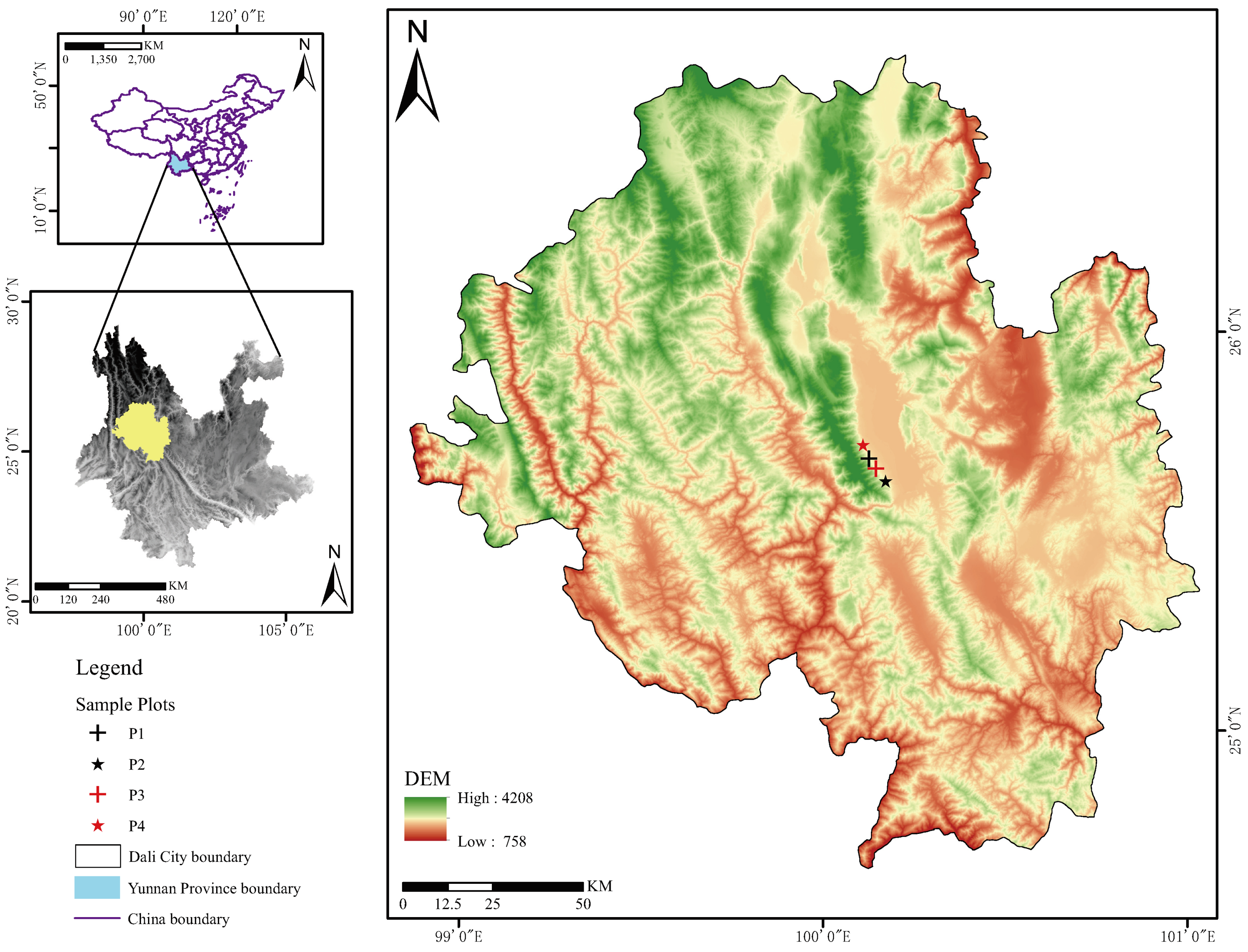
2.1. Study Areas
2.2. Study Site and Data Collection
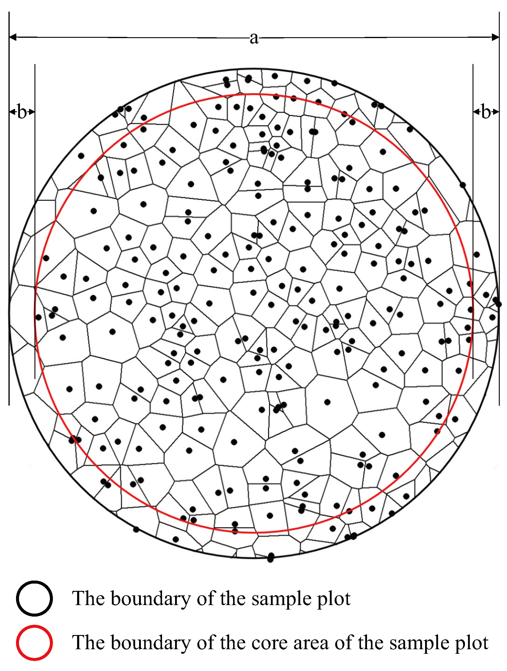
2.3. Determination of Spatial Structure Units and Edge Correction
2.4. Stand Structure Indexes
Spatial Structure Indexes
2.5. Methods for Selecting Trees for Cutting
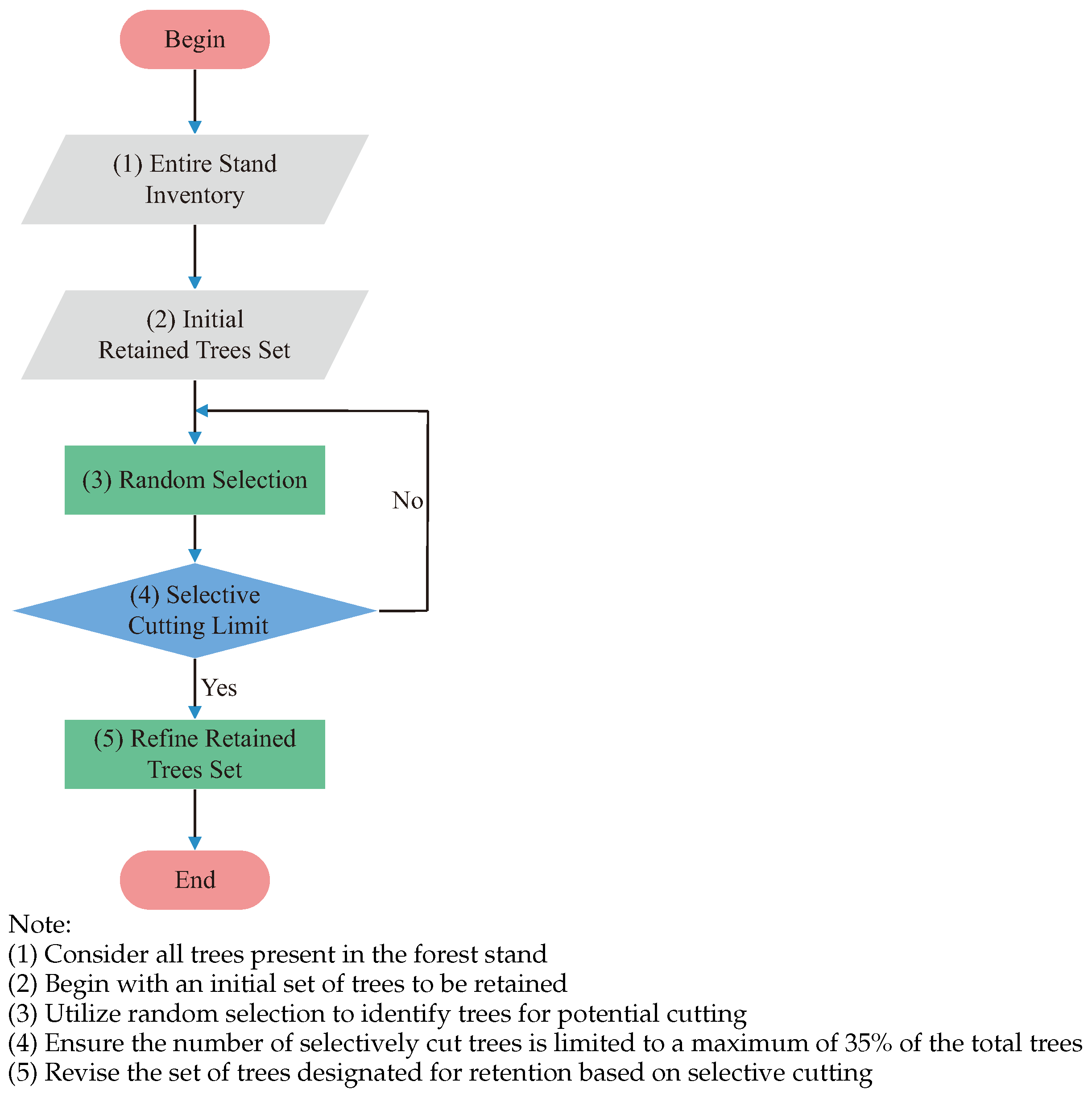
2.5.1. RSM (Random Selection Method) [20]
2.5.2. QVM (Q-Value Method) [21]
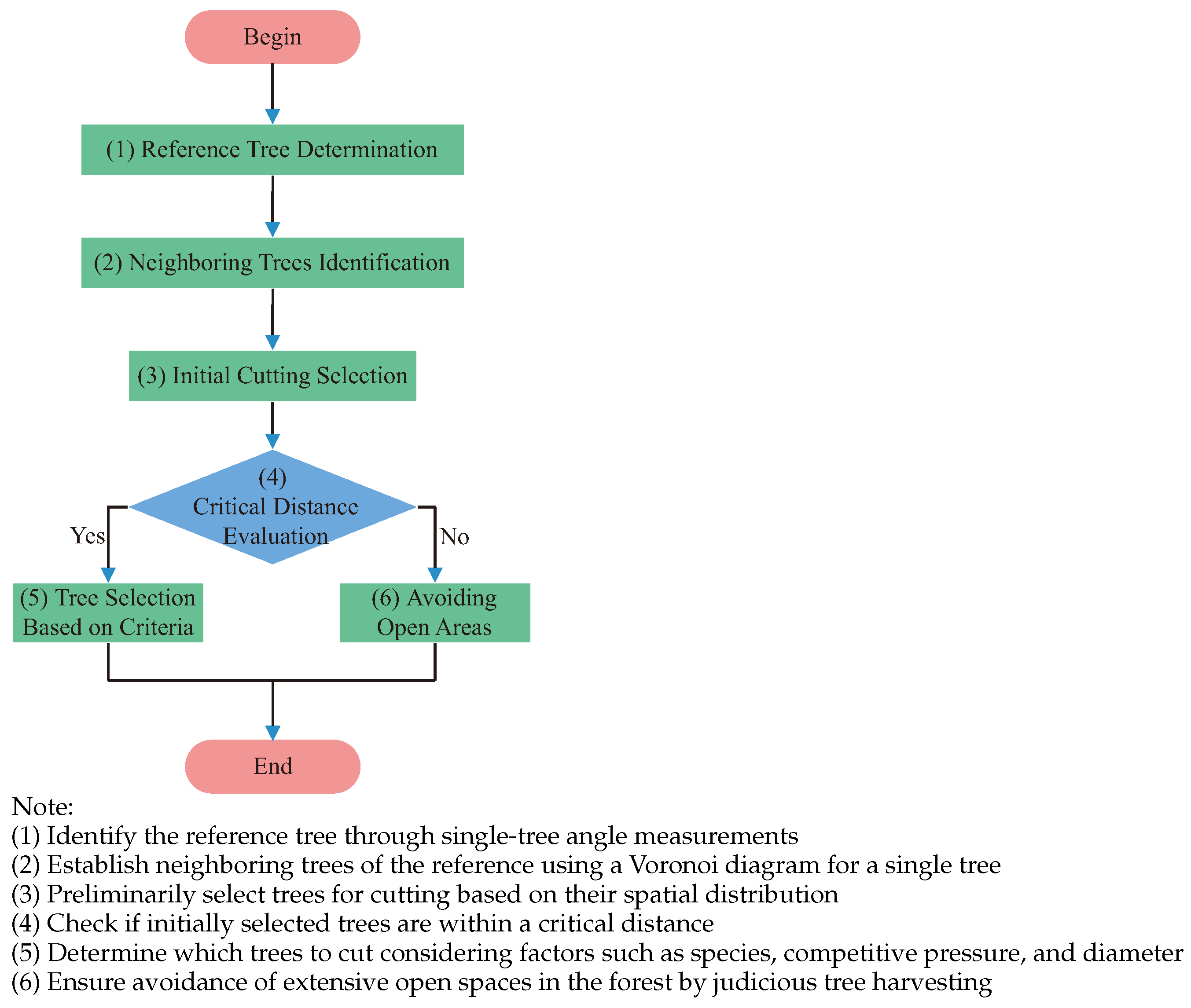
2.5.3. VMM (V-Map Method) [22]
2.6. Optimization Model for Selection Cutting of Forest Stand Structure
2.6.1. Constraints
2.6.2. Construction of the Model
2.7. Algorithms for Solving the Model
2.7.1. MC (Monte Carlo)
2.7.2. PSO (Particle Swarm Optimization)
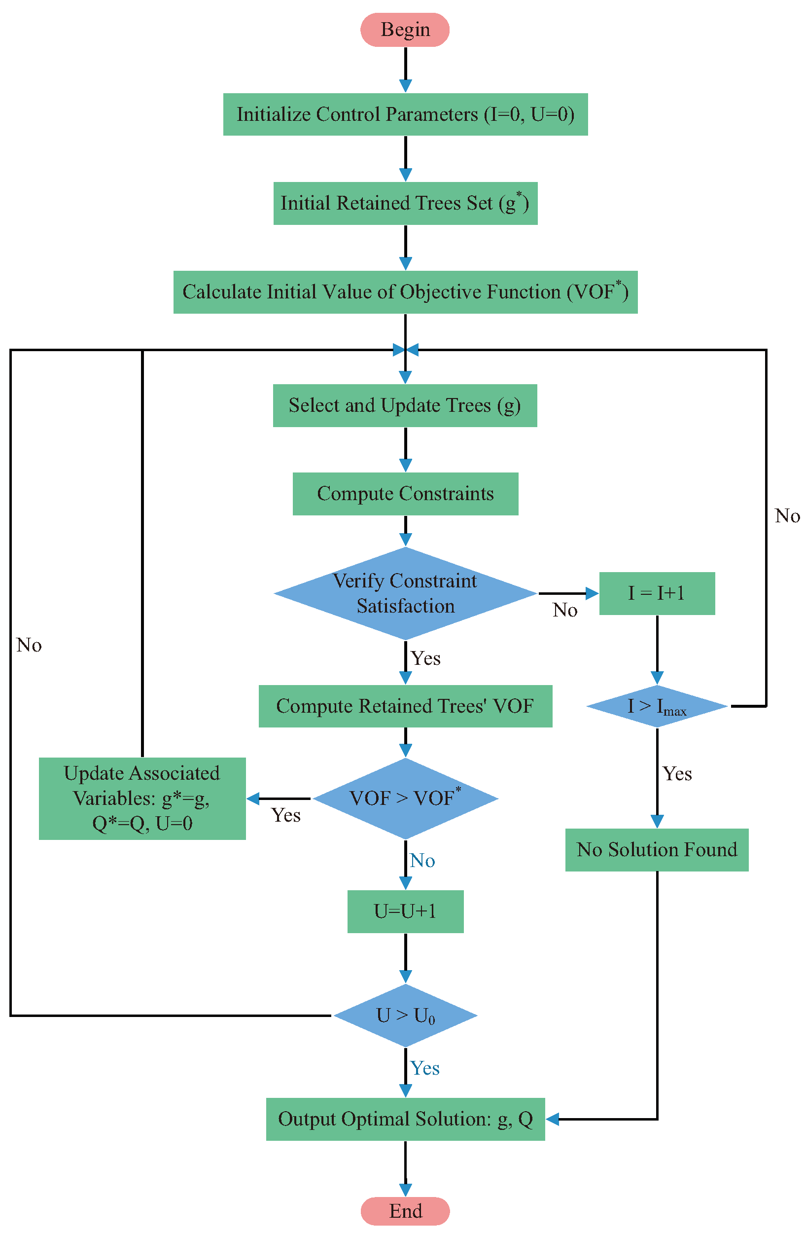
2.7.3. RL (Reinforcement Learning)
2.7.4. Optimization Schemes
3. Results
3.1. Algorithm Parameter Settings
3.2. Results of Simulated Selective Cutting Optimization
3.3. Algorithm Performance
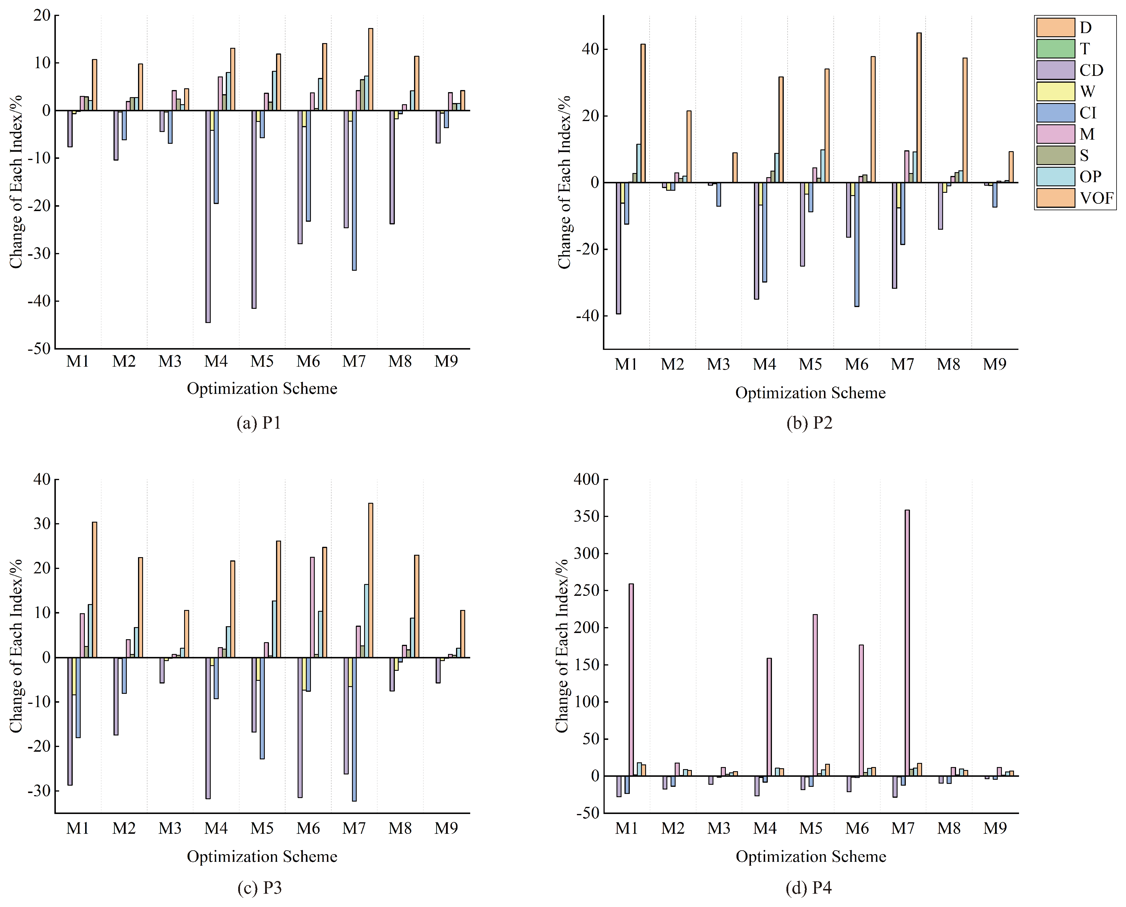
3.4. Influence of Proposed Selective Felling Tree Determination Methods
4. Discussion
4.1. Results of Simulated Selective Cutting Optimization
4.2. Algorithm Performance
4.3. Influence of Proposed Selective Felling Tree Determination Methods
5. Conclusions
Author Contributions
Funding
Data Availability Statement
Conflicts of Interest
Appendix A
| Algorithm A1: RL for MOFSS |
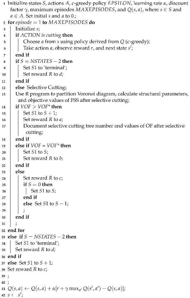 |
Appendix B
Appendix B.1
Appendix B.2

References
- Sun, H.L.; Li, S.C.; Xiong, W.L.; Yang, Z.R.; Cui, B.S. Influence of slope on root system anchorage of Pinus yunnanensis. Ecol. Eng. 2008, 32, 60–67. [Google Scholar] [CrossRef]
- Jin, Z.; Peng, J. Yunnan Pine (Pinus yunnanensis franch.); Yunnan Science and Technology Press: Kunming, China, 2004; pp. 1–66. [Google Scholar]
- Xu, Y.; Woeste, K.; Cai, N.; Kang, X.; Li, G.; Chen, S.; Duan, A. Variation in needle and cone traits in natural populations of Pinusyunnanensis. J. For. Res. 2015, 27, 41–49. [Google Scholar] [CrossRef]
- Sinicae, I.B.K.A. Flora Yunnanica. Tomus 6. (Spermatophyta); Wu, C.Y., Ed.; Science Press: Beijing, China, 1995; p. 759. [Google Scholar]
- Deng, W.; Xiang, W.; Ouyang, S.; Hu, Y.; Chen, L.; Zeng, Y.; Deng, X.; Zhao, Z.; Forrester, D.I. Spatially explicit optimization of the forest management tradeoff between timber production and carbon sequestration. Ecol. Indic. 2022, 142, 109193. [Google Scholar] [CrossRef]
- Jiang, L.; Lu, Y.C.; Liao, S.X.; Li, K.; Li, G.Q. A study on diameteral structure of Yunnan pine forest in the plateaus of mid-Yunnan Province. For. Res. 2008, 21, 126–130. [Google Scholar]
- Zaizhi, Z. Status and perspectives on secondary forests in tropical China. J. Trop. For. Sci. 2001, 2001, 639–651. [Google Scholar]
- Li, L.F.; Han, M.Y.; Zheng, W.; Su, J.W.; Li, W.C.; Zheng, S.H.; Gong, J.B. The causes of formation of low quality forest of Pinus yunnanensis and their classification. J. West China For. Sci. 2009, 38, 94–99. [Google Scholar]
- Yuan, R.; Yang, S.; Wang, B. Study on the altitudinal pattern of vegetation distribution along the eastern slope of Cangshan Mountain, Yunnan. China. J. Yunnan Univ. 2008, 30, 318–325. [Google Scholar]
- de Lima, R.A.F.; Batista, J.L.F.; Prado, P.I. Modeling tree diameter distributions in natural forests: An evaluation of 10 statistical models. For. Sci. 2015, 61, 320–327. [Google Scholar] [CrossRef]
- Abdollahnejad, A.; Panagiotidis, D.; Surovỳ, P. Forest canopy density assessment using different approaches—Review. J. For. Sci. 2017, 63, 107–116. [Google Scholar] [CrossRef]
- Petritan, A.M.; Biris, I.A.; Merce, O.; Turcu, D.O.; Petritan, I.C. Structure and diversity of a natural temperate sessile oak (Quercus petraea L.)—European Beech (Fagus sylvatica L.) forest. For. Ecol. Manag. 2012, 280, 140–149. [Google Scholar] [CrossRef]
- Bettinger, P.; Tang, M. Tree-level harvest optimization for structure-based forest management based on the species mingling index. Forests 2015, 6, 1121–1144. [Google Scholar] [CrossRef]
- Bao, Q.; Liang, X.W.; Weng, G.S. The Concept of Tree Crown Overlap and its Calculating Methods of Area. J. Northeast For. Univ. 1995, 23, 103–109. [Google Scholar]
- Wang, J.M. Study on Decision Technology of Tending Felling for Larix Principis-Rupprechtii Plantation Forest. Ph.D. Thesis, Beijing Forestry University, Beijing, China, 2017. [Google Scholar]
- Zhang, G.; Hui, G.; Zhao, Z.; Hu, Y.; Wang, H.; Liu, W.; Zang, R. Composition of basal area in natural forests based on the uniform angle index. Ecol. Inform. 2018, 45, 1–8. [Google Scholar] [CrossRef]
- Wan, P.; Zhang, G.; Wang, H.; Zhao, Z.; Hu, Y.; Zhang, G.; Hui, G.; Liu, W. Impacts of different forest management methods on the stand spatial structure of a natural Quercus aliena var. acuteserrata forest in Xiaolongshan, China. Ecol. Inform. 2019, 50, 86–94. [Google Scholar] [CrossRef]
- Yong, L.; Hao, Z.; Xianjun, W.; Zhiang, D.; Jianjun, L. Storey structure study of Cyclobalanopsis myrsinaefolia mixed stand based on storey index. For. Resour. Manag. 2012, 81–84. [Google Scholar]
- Joshi, C.; De Leeuw, J.; Skidmore, A.K.; Van Duren, I.C.; Van Oosten, H. Remotely sensed estimation of forest canopy density: A comparison of the performance of four methods. Int. J. Appl. Earth Obs. Geoinf. 2006, 8, 84–95. [Google Scholar] [CrossRef]
- Tang, M.P.; Tang, S.Z.; Lei, X.D.; Li, X.F. Study on Spatial Structure Optimizing Model of Stand Selection Cutting. Sci. Silvae Sin. 2004, 40, 25–31. [Google Scholar]
- Yu, Y.T. Study on Forest Structure of Different Recovery Stages and Optimization Models of Natural Mixed Spruce-fir Secondary Forests on Selective Cutting. Ph.D. Thesis, Beijing Forestry University, Beijing, China, 2019. [Google Scholar]
- Hao, Y.L. Study on Cutting Tree Determining Method Based on Forest Stand Spatial Structure Optimization. Ph.D. Thesis, Chinese Academy of Forestry, Beijing, China, 2012. [Google Scholar]
- Nelson, J.; Finn, S. The influence of cut-block size and adjacency rules on harvest levels and road networks. Can. J. For. Res. 1991, 21, 595–600. [Google Scholar] [CrossRef]
- Haight, R.G.; Travis, L.E. Wildlife conservation planning using stochastic optimization and importance sampling. For. Sci. 1997, 43, 129–139. [Google Scholar]
- Barrett, T.; Gilless, J.; Davis, L. Economic and fragmentation effects of clearcut restrictions. For. Sci. 1998, 44, 569–577. [Google Scholar]
- Boston, K.; Bettinger, P. An analysis of Monte Carlo integer programming, simulated annealing, and tabu search heuristics for solving spatial harvest scheduling problems. For. Sci. 1999, 45, 292–301. [Google Scholar]
- Okasha, N.M.; Frangopol, D.M. Lifetime-oriented multi-objective optimization of structural maintenance considering system reliability, redundancy and life-cycle cost using GA. Struct. Saf. 2009, 31, 460–474. [Google Scholar] [CrossRef]
- Singh, H.K.; Ray, T.; Smith, W. Surrogate assisted simulated annealing (SASA) for constrained multi-objective optimization. In Proceedings of the IEEE Congress on Evolutionary Computation, Barcelona, Spain, 18–23 July 2010; pp. 1–8. [Google Scholar]
- Cakir, B.; Altiparmak, F.; Dengiz, B. Multi-objective optimization of a stochastic assembly line balancing: A hybrid simulated annealing algorithm. Comput. Ind. Eng. 2011, 60, 376–384. [Google Scholar] [CrossRef]
- Liu, C.A. Research on Dynamic Multiobjective Optimization Evolutionary Algorithms. Nat. Sci. J. Hainan Univ. 2010, 28, 176–182. [Google Scholar]
- Zhang, Y.; Gong, D.w.; Ding, Z.h. Handling multi-objective optimization problems with a multi-swarm cooperative particle swarm optimizer. Expert Syst. Appl. 2011, 38, 13933–13941. [Google Scholar] [CrossRef]
- Hu, C.Y.; Yao, H.; Yan, X.S. Multiple Particle Swarms Coevolutionary Algorithm for Dynamic Multi-Objective Optimization Problems and Its Application. J. Comput. Res. Dev. 2013, 50, 1313–1323. [Google Scholar]
- Biswas, D.; Panja, S.; Guha, S. Multi objective optimization method by PSO. Procedia Mater. Sci. 2014, 6, 1815–1822. [Google Scholar] [CrossRef]
- Gunantara, N. A review of multi-objective optimization: Methods and its applications. Cogent Eng. 2018, 5, 1502242. [Google Scholar] [CrossRef]
- Moore, C.T.; Conroy, M.J.; Boston, K. Forest management decisions for wildlife objectives: System resolution and optimality. Comput. Electron. Agric. 2000, 27, 25–39. [Google Scholar] [CrossRef]
- Levine, S.; Finn, C.; Darrell, T.; Abbeel, P. End-to-end training of deep visuomotor policies. J. Mach. Learn. Res. 2016, 17, 1334–1373. [Google Scholar]
- Wiering, M.A.; Van Otterlo, M. Reinforcement learning. Adapt. Learn. Optim. 2012, 12, 729. [Google Scholar]
- Sutton, R.S.; Barto, A.G. Reinforcement Learning: An Introduction; MIT Press: Cambridge, MA, USA, 2018. [Google Scholar]
- Abels, A.; Roijers, D.; Lenaerts, T.; Nowé, A.; Steckelmacher, D. Dynamic weights in multi-objective deep reinforcement learning. In Proceedings of the International Conference on Machine Learning, PMLR, Long Beach, CA, USA, 9–15 June 2019; pp. 11–20. [Google Scholar]
- Zou, F.; Yen, G.G.; Tang, L.; Wang, C. A reinforcement learning approach for dynamic multi-objective optimization. Inf. Sci. 2021, 546, 815–834. [Google Scholar]
- Anderson, R.N.; Boulanger, A.; Powell, W.B.; Scott, W. Adaptive stochastic control for the smart grid. Proc. IEEE 2011, 99, 1098–1115. [Google Scholar] [CrossRef]
- Glavic, M.; Fonteneau, R.; Ernst, D. Reinforcement learning for electric power system decision and control: Past considerations and perspectives. IFAC-PapersOnLine 2017, 50, 6918–6927. [Google Scholar] [CrossRef]
- Haksar, R.N.; Schwager, M. Distributed deep reinforcement learning for fighting forest fires with a network of aerial robots. In Proceedings of the 2018 IEEE/RSJ International Conference on Intelligent Robots and Systems (IROS), Madrid, Spain, 1–5 December 2018; pp. 1067–1074. [Google Scholar]
- Moussa, N.; Nurellari, E.; Azbeg, K.; Boulouz, A.; Afdel, K.; Koutti, L.; Salah, M.B.; El Alaoui, A.E.B. A reinforcement learning based routing protocol for software-defined networking enabled wireless sensor network forest fire detection. Future Gener. Comput. Syst. 2023, 149, 478–493. [Google Scholar] [CrossRef]
- Tahvonen, O.; Suominen, A.; Malo, P.; Viitasaari, L.; Parkatti, V.P. Optimizing high-dimensional stochastic forestry via reinforcement learning. J. Econ. Dyn. Control. 2022, 145, 104553. [Google Scholar] [CrossRef]
- Malo, P.; Tahvonen, O.; Suominen, A.; Back, P.; Viitasaari, L. Reinforcement learning in optimizing forest management. Can. J. For. Res. 2021, 51, 1393–1409. [Google Scholar] [CrossRef]
- Shi, Y.; Xu, L.; Zhou, Y.; Ji, B.; Zhou, G.; Fang, H.; Yin, J.; Deng, X. Quantifying driving factors of vegetation carbon stocks of Moso bamboo forests using machine learning algorithm combined with structural equation model. For. Ecol. Manag. 2018, 429, 406–413. [Google Scholar] [CrossRef]
- Liu, Z.; Peng, C.; Work, T.; Candau, J.N.; DesRochers, A.; Kneeshaw, D. Application of machine-learning methods in forest ecology: Recent progress and future challenges. Environ. Rev. 2018, 26, 339–350. [Google Scholar] [CrossRef]
- Pang, Y.; Li, Y.; Feng, Z.; Feng, Z.; Zhao, Z.; Chen, S.; Zhang, H. Forest fire occurrence prediction in China based on machine learning methods. Remote Sens. 2022, 14, 5546. [Google Scholar] [CrossRef]
- Silva, J.P.M.; da Silva, M.L.M.; de Mendonça, A.R.; da Silva, G.F.; de Barros Junior, A.A.; da Silva, E.F.; Aguiar, M.O.; Santos, J.S.; Rodrigues, N.M.M. Prognosis of forest production using machine learning techniques. Inf. Process. Agric. 2021, 10, 71–84. [Google Scholar]
- Neuville, R.; Bates, J.S.; Jonard, F. Estimating forest structure from UAV-mounted LiDAR point cloud using machine learning. Remote Sens. 2021, 13, 352. [Google Scholar] [CrossRef]
- Hamedianfar, A.; Mohamedou, C.; Kangas, A.; Vauhkonen, J. Deep learning for forest inventory and planning: A critical review on the remote sensing approaches so far and prospects for further applications. Forestry 2022, 95, 451–465. [Google Scholar] [CrossRef]
- Sani-Mohammed, A.; Yao, W.; Heurich, M. Instance segmentation of standing dead trees in dense forest from aerial imagery using deep learning. ISPRS Open J. Photogramm. Remote Sens. 2022, 6, 100024. [Google Scholar] [CrossRef]
- Liu, S. Research on the Analysis and Multi-objective Intelligent Optimization of Stand Structure of Natural Secondary Forest. Ph.D. Thesis, Central South University of Forestry and Technology, Changsha, China, 2017. [Google Scholar]
- Liao, J.; Li, Z.; Quets, J.J.; Nijs, I. Effects of space partitioning in a plant species diversity model. Ecol. Model. 2013, 251, 271–278. [Google Scholar] [CrossRef]
- Magnussen, S.; Allard, D.; Wulder, M.A. Poisson Voronoi tiling for finding clusters in spatial point patterns. Scand. J. For. Res. 2006, 21, 239–248. [Google Scholar] [CrossRef]
- Sterner, R.W.; Ribic, C.A.; Schatz, G.E. Testing for life historical changes in spatial patterns of four tropical tree species. J. Ecol. 1986, 74, 621–633. [Google Scholar] [CrossRef]
- Hui, G.Y.; Hu, Y.B.; Zhao, Z.H. Research progress of structure-based forest management. For. Res. 2018, 31, 85–93. [Google Scholar]
- Liu, S.; Zhang, J.; Li, J.J.; Zhou, G.X.; Wu, S.C. Edge Correction of Voronoi Diagram in Forest Spatial Structure Analysis. Sci. Silvae Sin. 2017, 53, 28–37. [Google Scholar]
- Xiang, B. Study on the Structure Adjustment and Optimization of Quercus Secondary Forest in Hunan Province. Master’s Thesis, Central South University of Forestry and Technology, Changsha, China, 2019. [Google Scholar]
- Su, J.W.; Li, L.F.; Zheng, W.; Yang, W.B.; Han, M.Y.; Huang, Z.M.; Xu, P.B.; Feng, Z.W. Effect of Intermediate Cutting Intensity on Growth of Pinus yunnanensis Plantation. J. West China For. Sci. 2010, 39, 27–32. [Google Scholar]
- Han, M.Y.; Li, L.F.; Zheng, W.; Su, J.W.; Li, W.C.; Gong, J.B.; Zheng, S.H. Effects of different intensity of thinning on the improvement of middle-aged Yunnan pine stand. J. Cent. South Univ. For. Technol. 2011, 31, 27–33. [Google Scholar]
- Zhang, G.; Hui, G.; Hu, Y.; Zhao, Z.; Guan, X.; von Gadow, K.; Zhang, G. Designing near-natural planting patterns for plantation forests in China. For. Ecosyst. 2019, 6, 1–13. [Google Scholar] [CrossRef]
- Johann, K. Der A-Wert ein objektiver Parameter zur Bestimmung der Freistellungsstärke von Zentralbäumen. Dtsch. Verb. Forstl. Forschungsanstalten–Sekt. Ertragskunde 1982, 25, 27. [Google Scholar]
- Huang, J. The Research on Dynamic Multi-objectives Optimization of Forest Space Based on multi-swarm PSO Algorithm. Master’s Thesis, Central South University of Forestry and Technology, Changsha, China, 2017. [Google Scholar]
- Li, J.J.; Li, J.P.; Liu, S.Q.; Zhang, H.W.; Feng, X.L. Homogeneity Index of Stand Spatial Structure of Mangrove Ecological System. Sci. Silvae Sin. 2010, 46, 6–14. [Google Scholar]
- Qing, D.; Peng, J.; Li, J.; Liu, S.; Deng, Q. Genetic algorithm to solve the optimization problem of stand spatial structure. J. For. Environ. 2022, 42, 434–441. [Google Scholar]
- Poudyal, B.H.; Maraseni, T.; Cockfield, G. Evolutionary dynamics of selective logging in the tropics: A systematic review of impact studies and their effectiveness in sustainable forest management. For. Ecol. Manag. 2018, 430, 166–175. [Google Scholar] [CrossRef]
- Ehbrecht, M.; Schall, P.; Ammer, C.; Seidel, D. Quantifying stand structural complexity and its relationship with forest management, tree species diversity and microclimate. Agric. For. Meteorol. 2017, 242, 1–9. [Google Scholar] [CrossRef]
- Silva, P.H.d.; Gomide, L.R.; Figueiredo, E.O.; Carvalho, L.M.T.d.; Ferraz-Filho, A.C. Optimal selective logging regime and log landing location models: A case study in the Amazon forest. Acta Amaz. 2018, 48, 18–27. [Google Scholar] [CrossRef]
- Cazzolla Gatti, R.; Castaldi, S.; Lindsell, J.A.; Coomes, D.A.; Marchetti, M.; Maesano, M.; Di Paola, A.; Paparella, F.; Valentini, R. The impact of selective logging and clearcutting on forest structure, tree diversity and above-ground biomass of African tropical forests. Ecol. Res. 2015, 30, 119–132. [Google Scholar] [CrossRef]
- Li, J.J.; Liu, S.; Zhang, H.R.; Kuang, Z.F.; Wang, C.L.; Zhang, J.; Cao, X.P. Heterogeneity evaluation of forest ecological system spatial structure in Dongting Lake. Acta Ecol. Sin. 2013, 33, 3732–3741. [Google Scholar]
- Li, N. The Research on Dynamic multi-objective optimization model of forest structure under CMIP5 model. Master’s Thesis, Central South University of Forestry and Technology, Changsha, China, 2019. [Google Scholar]
- Chen, Y.T.; Chang, C.T. Multi-coefficient goal programming in thinning schedules to increase carbon sequestration and improve forest structure. Ann. For. Sci. 2014, 71, 907–915. [Google Scholar] [CrossRef]
- Zhou, C.; Wu, Z.; Zhou, X.; Zeng, H.; Zeng, L. Impact of Cutting Intensity on Forest Stand Growth and Understand Species Diversity of the Mixed Plantations of Cunninghamia lancelata and Broadleaved Trees. For. Eng. 2023, 39, 46–53. [Google Scholar]
- Alsuwaiyel, M.H. Algorithms: Design Techniques and Analysis; World Scientific: Singapore, 2021; Volume 15. [Google Scholar]
- Zenil, H. A review of methods for estimating algorithmic complexity: Options, challenges, and new directions. Entropy 2020, 22, 612. [Google Scholar] [CrossRef] [PubMed]
- Oliveto, P.S.; Witt, C. Improved time complexity analysis of the simple genetic algorithm. Theor. Comput. Sci. 2015, 605, 21–41. [Google Scholar] [CrossRef]
- Roy, V. Convergence diagnostics for markov chain monte carlo. Annu. Rev. Stat. Its Appl. 2020, 7, 387–412. [Google Scholar] [CrossRef]
- Sobol, I.M. A Primer for the Monte Carlo Method; CRC Press: Boca Raton, FL, USA, 2018. [Google Scholar]
- Zio, E.; Zio, E. Monte Carlo Simulation: The Method; Springer: Cham, Switzerland, 2013. [Google Scholar]
- Szepesvári, C. Algorithms for Reinforcement Learning; Springer Nature: Berlin/Heidelberg, Germany, 2022. [Google Scholar]
- Shresthamali, S.; Kondo, M.; Nakamura, H. Multi-Objective Resource Scheduling for IoT Systems Using Reinforcement Learning. J. Low Power Electron. Appl. 2022, 12, 53. [Google Scholar] [CrossRef]
- Fang, M.; Li, Y.; Cohn, T. Learning how to active learn: A deep reinforcement learning approach. arXiv 2017, arXiv:1708.02383. [Google Scholar]
- Jain, M.; Saihjpal, V.; Singh, N.; Singh, S.B. An overview of variants and advancements of PSO algorithm. Appl. Sci. 2022, 12, 8392. [Google Scholar] [CrossRef]
- Jordehi, A.R. Enhanced leader PSO (ELPSO): A new PSO variant for solving global optimisation problems. Appl. Soft Comput. 2015, 26, 401–417. [Google Scholar] [CrossRef]
- Rubinstein, R.Y.; Kroese, D.P. Simulation and the Monte Carlo Method; John Wiley & Sons: Hoboken, NJ, USA, 2016. [Google Scholar]
- Botvinick, M.; Ritter, S.; Wang, J.X.; Kurth-Nelson, Z.; Blundell, C.; Hassabis, D. Reinforcement learning, fast and slow. Trends Cogn. Sci. 2019, 23, 408–422. [Google Scholar] [CrossRef]
- Garg, H. A hybrid PSO-GA algorithm for constrained optimization problems. Appl. Math. Comput. 2016, 274, 292–305. [Google Scholar] [CrossRef]
- Das, H.; Jena, A.K.; Nayak, J.; Naik, B.; Behera, H. A novel PSO based back propagation learning-MLP (PSO-BP-MLP) for classification. In Computational Intelligence in Data Mining-Volume 2: Proceedings of the International Conference on CIDM, 20–21 December 2014; Springer: New Delhi, India, 2015; pp. 461–471. [Google Scholar]
- Bansal, J.C. Particle swarm optimization. In Evolutionary and Swarm Intelligence Algorithms; Springer: Cham, Switzerland, 2019; pp. 11–23. [Google Scholar]
- Stephens, S.L.; Lydersen, J.M.; Collins, B.M.; Fry, D.L.; Meyer, M.D. Historical and current landscape-scale ponderosa pine and mixed conifer forest structure in the Southern Sierra Nevada. Ecosphere 2015, 6, 1–63. [Google Scholar] [CrossRef]


| Sample Plots | East Long. | North Lat. | Elevation (m) | Slope () | Slope Dir. | Sample Plot Radius (m) | Tree Species Composition | Stand Density (Trees/ha) |
|---|---|---|---|---|---|---|---|---|
| P1 | 100°08.2149 | 25°41.5280 | 2254 | 13.45 | East | 35 | 8 PY-2 PA-BA-TG | 1481 |
| P2 | 100°10.9639 | 25°38.1518 | 2271 | 16.15 | South | 32 | 7 PY-3 PA | 1822 |
| P3 | 100°09.3947 | 25°39.9506 | 2195 | 17.70 | NE | 20 | 7 PY-3 PA-QA-VB GG-BA | 1830 |
| P4 | 100°07.1906 | 25°43.5923 | 2138 | 5.10 | NE | 19 | 10 PY-QA | 1975 |
| RSM | QVM | VMM | |
|---|---|---|---|
| MC | r-MC(M1) | Q-MC(M2) | V-MC(M3) |
| PSO | r-PSO(M4) | Q-PSO(M5) | V-PSO(M6) |
| RL | r-RL(M7) | Q-RL(M8) | V-RL(M9) |
| Algorithms | Parameters and Parameter Values | Value Meaning |
|---|---|---|
| MC | Initial iteration | |
| = 10,000 | Maximum number of iterations | |
| Initial number of consecutive iterations without OF improvement | ||
| Maximum number of consecutive iterations without OF improvement | ||
| PSO | Initial iteration | |
| = 10,000 | Maximum number of iterations | |
| Number of particles | ||
| Inertia weights | ||
| Individual particle learning factor | ||
| Global learning factor | ||
| RL | Initial iteration | |
| = 10,000 | Maximum number of iterations | |
| Initial position of the agent | ||
| Farthest position the agent is allowed to move to | ||
| , , , | Reward and penalty values |
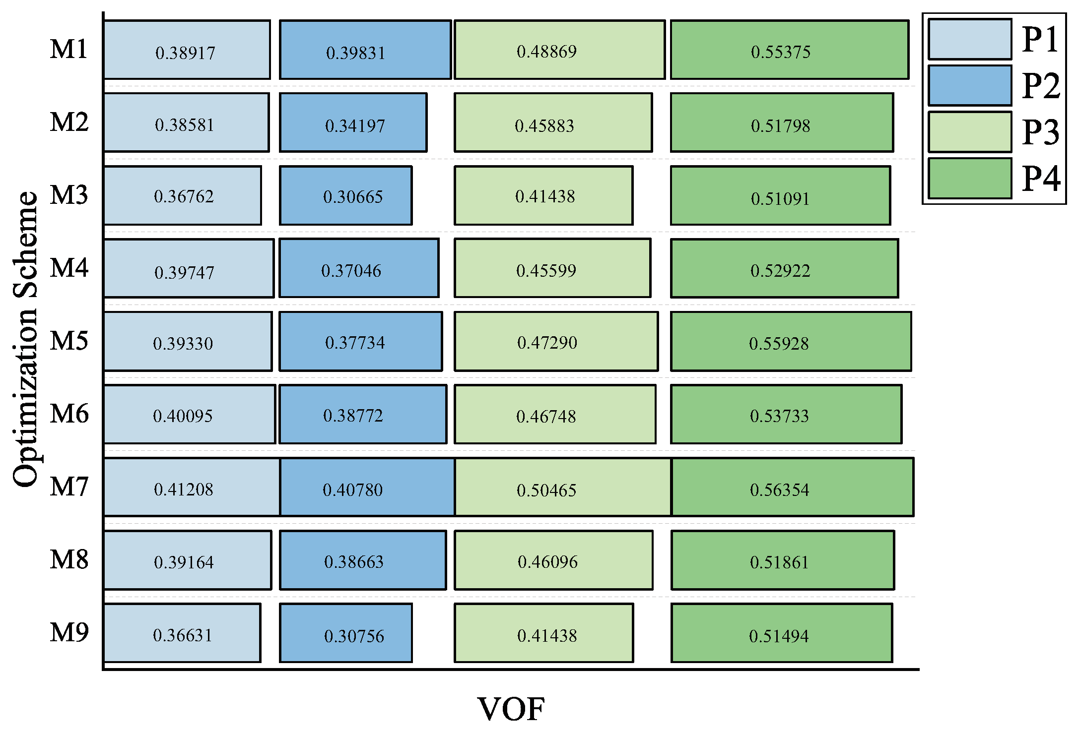
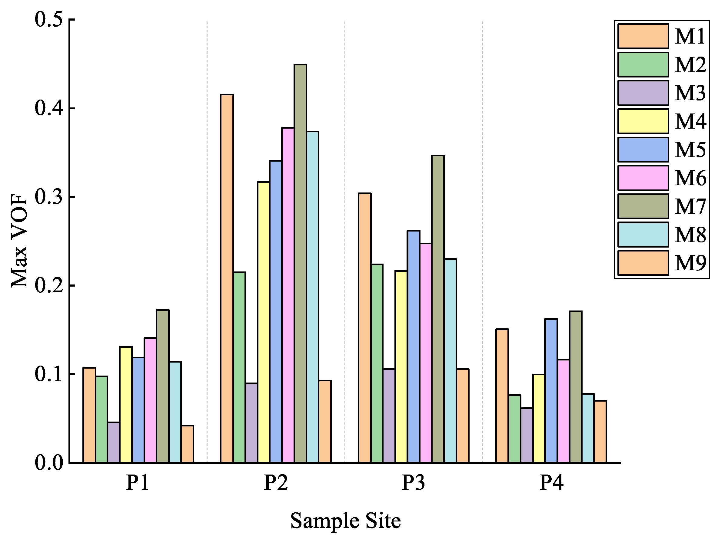
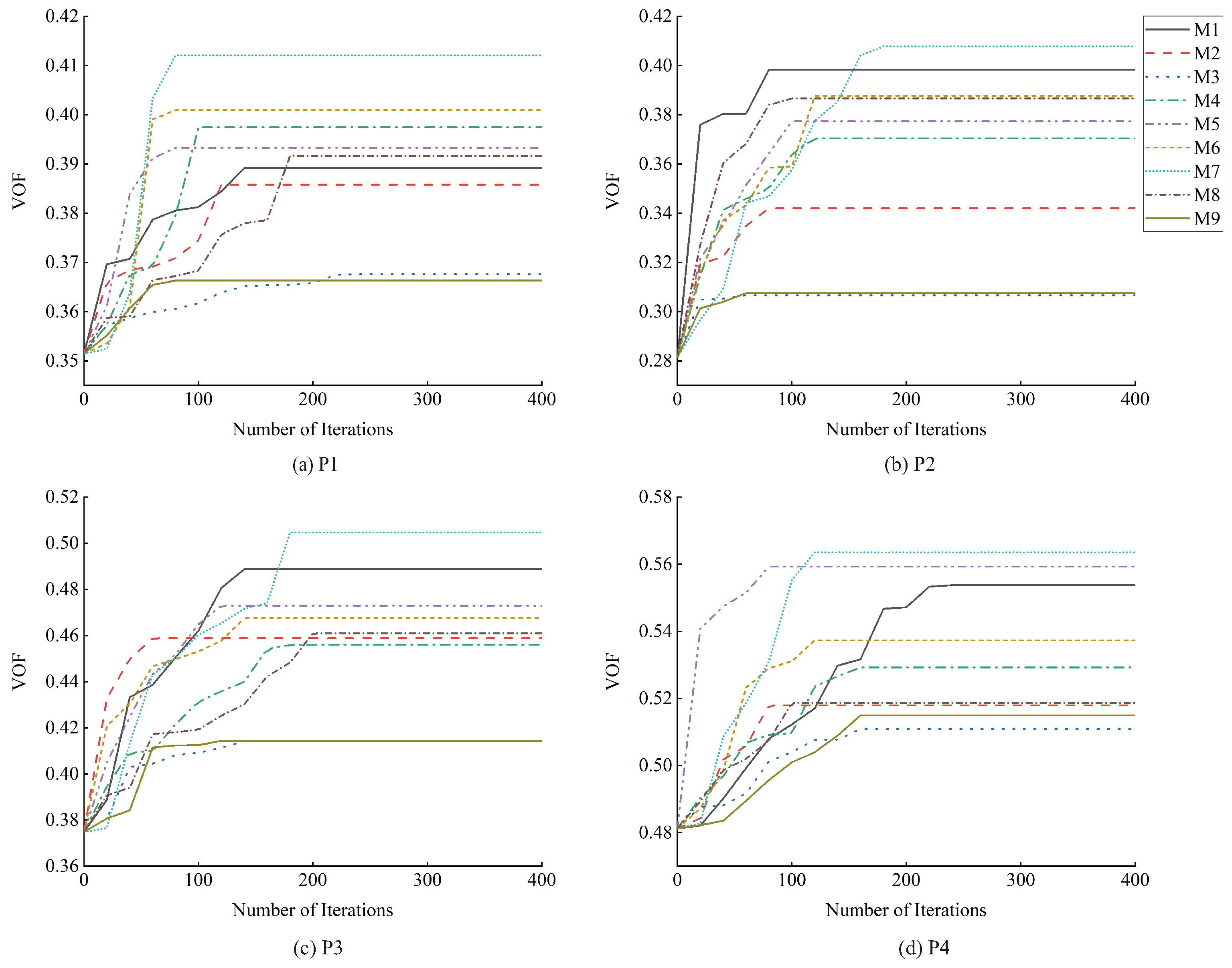
| VOF | P1 | P2 | P3 | P4 | Average Value of Scheme | Improvement Magnitude of Scheme | Average Improvement Magnitude of Scheme | |
|---|---|---|---|---|---|---|---|---|
| Before Cutting | 0.3515 | 0.2814 | 0.3748 | 0.4812 | 0.3722 | |||
| After Cutting | M1 | 0.3892 | 0.3983 | 0.4887 | 0.5537 | 0.4575 | 22.92% | 17.42% |
| M2 | 0.3858 | 0.3420 | 0.4588 | 0.5180 | 0.4261 | 14.48% | ||
| M3 | 0.3676 | 0.3066 | 0.4144 | 0.5109 | 0.3999 | 7.44% | ||
| M4 | 0.3975 | 0.3705 | 0.4560 | 0.5292 | 0.4383 | 17.76% | ||
| M5 | 0.3933 | 0.3773 | 0.4729 | 0.5593 | 0.4507 | 21.09% | ||
| M6 | 0.4009 | 0.3877 | 0.4675 | 0.5373 | 0.4484 | 20.47% | ||
| M7 | 0.4121 | 0.4078 | 0.5047 | 0.5635 | 0.4720 | 26.81% | ||
| M8 | 0.3916 | 0.3866 | 0.4610 | 0.5186 | 0.4395 | 18.08% | ||
| M9 | 0.3663 | 0.3076 | 0.4144 | 0.5149 | 0.4008 | 7.684% | ||
| Average Value of Sample Plot | 0.3894 | 0.3649 | 0.4598 | 0.5340 | ||||
| Running Time/(min) | M1 | M2 | M3 | M4 | M5 | M6 | M7 | M8 | M9 |
|---|---|---|---|---|---|---|---|---|---|
| P1 | 7847.881 | 4997.854 | 9793.233 | 4198.420 | 3404.310 | 3401.141 | 3398.441 | 7394.313 | 3400.292 |
| P2 | 4845.591 | 3450.688 | 2635.718 | 5053.131 | 4240.855 | 5058.874 | 7229.825 | 4242.174 | 2641.545 |
| P3 | 7892.756 | 2645.365 | 6600.294 | 7424.275 | 5039.715 | 5039.071 | 7372.265 | 8207.307 | 5007.491 |
| P4 | 12,947.977 | 3475.821 | 6615.058 | 6632.085 | 3459.199 | 5033.976 | 5035.914 | 4242.309 | 6626.676 |
| Sample Site | Optimal Scheme | Tree Number | DBH (cm) | TH (m) | CW (m) | Tree Specie |
|---|---|---|---|---|---|---|
| P1 | M7 | 76 | 11.90 | 10.40 | 1.43 | PY |
| M7 | 234 | 7.80 | 7.20 | 1.78 | PA | |
| M7 | 335 | 11.70 | 15.00 | 1.35 | PY | |
| M7 | 519 | 14.80 | 12.40 | 1.85 | PY | |
| M7 | 638 | 9.70 | 10.52 | 1.15 | PY | |
| P2 | M7 | 66 | 15.50 | 7.80 | 1.95 | PY |
| M7 | 224 | 10.50 | 7.50 | 1.43 | PY | |
| M7 | 319 | 8.50 | 5.70 | 2.08 | PA | |
| M7 | 505 | 5.00 | 4.10 | 1.10 | PY | |
| M7 | 670 | 19.40 | 12.75 | 2.25 | PY | |
| P3 | M7 | 61 | 22.10 | 15.85 | 1.75 | PY |
| M7 | 143 | 16.00 | 13.27 | 1.45 | PY | |
| M7 | 160 | 7.30 | 6.40 | 1.26 | PY | |
| M7 | 275 | 9.40 | 8.67 | 1.24 | PY | |
| M7 | 299 | 13.20 | 7.36 | 2.10 | PY | |
| P4 | M7 | 19 | 8.32 | 7.67 | 0.93 | PY |
| M7 | 68 | 7.70 | 6.27 | 1.19 | PY | |
| M7 | 145 | 22.80 | 11.20 | 1.93 | PY | |
| M7 | 194 | 5.62 | 6.50 | 1.58 | PY | |
| M7 | 247 | 16.15 | 11.56 | 2.00 | PY |
Disclaimer/Publisher’s Note: The statements, opinions and data contained in all publications are solely those of the individual author(s) and contributor(s) and not of MDPI and/or the editor(s). MDPI and/or the editor(s) disclaim responsibility for any injury to people or property resulting from any ideas, methods, instructions or products referred to in the content. |
© 2023 by the authors. Licensee MDPI, Basel, Switzerland. This article is an open access article distributed under the terms and conditions of the Creative Commons Attribution (CC BY) license (https://creativecommons.org/licenses/by/4.0/).
Share and Cite
Xuan, S.; Wang, J.; Chen, Y. Reinforcement Learning for Stand Structure Optimization of Pinus yunnanensis Secondary Forests in Southwest China. Forests 2023, 14, 2456. https://doi.org/10.3390/f14122456
Xuan S, Wang J, Chen Y. Reinforcement Learning for Stand Structure Optimization of Pinus yunnanensis Secondary Forests in Southwest China. Forests. 2023; 14(12):2456. https://doi.org/10.3390/f14122456
Chicago/Turabian StyleXuan, Shuai, Jianming Wang, and Yuling Chen. 2023. "Reinforcement Learning for Stand Structure Optimization of Pinus yunnanensis Secondary Forests in Southwest China" Forests 14, no. 12: 2456. https://doi.org/10.3390/f14122456
APA StyleXuan, S., Wang, J., & Chen, Y. (2023). Reinforcement Learning for Stand Structure Optimization of Pinus yunnanensis Secondary Forests in Southwest China. Forests, 14(12), 2456. https://doi.org/10.3390/f14122456