QPWS Feature Selection and CAE Fusion of Visible/Near-Infrared Spectroscopy Data for the Identification of Salix psammophila Origin

Abstract

Salix psammophila, classified under the Salicaceae family, is a deciduous, densely branched, and erect shrub. As a leading pioneer tree species in windbreak and sand stabilization, it has played a crucial role in combating desertification in northwestern China. However, different genetic sources of Salix psammophila exhibit significant variations in their effectiveness for windbreak and sand stabilization. Therefore, it is essential to establish a rapid and reliable method for identifying different Salix psammophila varieties. Visible and near-infrared (Vis-NIR) spectroscopy is currently a reliable non-destructive solution for origin traceability. This study introduced a novel feature selection strategy, called qualitative percentile weighted sampling (QPWS), based on the principle of the long tail effect for Vis-NIR spectroscopy. The core idea of QPWS combines weighted sampling and percentage wavelength selection to identify key wavelengths. By employing a multi-threaded parallel execution of multiple QPWS instances, we aimed to search for the optimal feature bands to address the instability issues that can arise during the feature selection process. To address the problem of reduced prediction performance in one-dimensional convolutional neural network (1D-CNN) models after feature selection, we have introduced convolutional autoencoders (CAEs) to reduce the dimensions of wavelengths that are discarded during feature selection. Subsequently, these reduced dimensions are fused with the selected wavelengths, thereby enhancing the model’s performance. With our completed model, we selected outstanding models for model fusion and established a decision system for Salix psammophila. It is worth noting that all 1D-CNN models in this study were developed using Bayesian optimization methods. In comparison with principal component analysis (PCA) and full spectrum methods, QPWS exhibits superior predictive performance in the field of machine learning. In the realm of deep learning, the fusion of data combining QPWS with CAE demonstrated even greater potential with an improvement of average accuracy of approximately 2.13% when compared to QPWS alone and a 228% increase in operational speed compared to a model with full spectra. These results indicated that the combination of CAE with QPWS can be an effective tool for identifying the origin of Salix psammophila.

1. Introduction

Desertification poses a severe threat to arid and semi-arid environments, which constitute approximately 41% of the global land area. Despite China’s efforts to combat desertification, it continues to persist. According to statistics, the total area of desertified land in China has reached 257,371,300 hectares (Figure 1) [1], accounting for 26.81% of the country’s total land area. This phenomenon predominantly affects regions such as Inner Mongolia, Gansu, Tibet, Xinjiang, and Qinghai, posing a significant threat to China’s ecological environment and agriculture [2]. Salix psammophila, a deciduous, bushy, and upright shrub belonging to the willow family (Salicaceae) [3], plays a vital role in windbreak and sand fixation in China. It exhibits cold, drought, high-temperature, and sand burial resistance, demonstrating strong adaptability, rapid growth, and a high tolerance for various environmental conditions. However, different genetic sources of Salix psammophila exhibit significant variations in their windbreak and sand-fixation capabilities [4]. To more effectively address desertification issues and implement scientific desertification control measures, the precise origin traceability of Salix psammophila is of utmost importance [5].

In recent years, Vis-NIR technology [6] has garnered widespread attention due to its numerous advantages including ease of operation, fast analysis, non-destructiveness, and cost effectiveness [7,8,9]. It has been widely adopted in various fields, becoming a popular tool for qualitative and quantitative analysis. However, with the continuous advancement of modern analytical instruments, Vis-NIR spectral data have become more comprehensive and cover a broader range of wavelengths. These high-dimensional data inevitably give rise to the ‘curse of dimensionality’ [10,11], where data dimensionality increases sharply, leading to complexity and unnecessary information redundancy. This issue poses a series of challenges to the data analysis and modeling process, one of which is the problem of multicollinearity [12]. Multicollinearity significantly increases the complexity of model interpretation and prediction. When addressing the challenges of high-dimensional data, feature selection, as a key technique, aims to eliminate redundant information, thereby reducing the dataset’s dimensionality and improving model efficiency [13,14,15,16].

Feature selection methods have seen widespread application, with the primary focus primarily concentrated in the quantitative analysis domain [17,18]. In qualitative analysis, the use of feature selection methods is relatively less common, and the more prevalent practice involves the utilization of dimension reduction techniques, such as PCA [19] and the successive projections algorithm (SPA) [20,21,22]. Dimensionality reduction techniques have a distinct advantage in terms of operational speed compared to feature selection. By focusing on the compression of independent variables in data calculations, they can rapidly reduce dimensions and automatically eliminate redundant wavelengths that do not provide significant information. This simplifies models and enhances computational efficiency. However, compared to feature selection, they often fall short in addressing two critical issues: model interpretability and accuracy, which are equally crucial in qualitative analysis [23,24,25]. Feature selection has an advantage in preserving wavelengths strongly correlated with the target attributes, aiding in improving the physical interpretability of the model. This makes the results more easily interpretable and aligns better with the relationship between the nature of the samples and the selected features. In the realm of qualitative analysis, the absence of suitable feature selection methods could potentially serve as a bottleneck, limiting the capability to accurately identify and classify various substances.

The core challenge of feature selection lies in the need to enhance operational speed while ensuring that the selected feature set effectively captures the essential information within the data [26]. When addressing this balance between speed and efficacy, machine learning evaluation methods are typically employed because machine learning algorithms are often faster and more efficient in feature selection [27]. Important bands were rapidly screened through cross-validation and correlation ranking. However, when dealing with relatively small datasets, deep learning typically does not require a separate feature selection step. This is because deep learning can automatically extract features from raw data; however, adopting strategies biased toward traditional machine learning can sometimes result in the selected feature set being insufficient to meet the requirements of deep learning algorithms, potentially diminishing the performance of deep learning models. There are generally two approaches to tackling this issue. One approach is to employ feature selection methods within deep learning; for instance, some researchers have used attention mechanisms, training attention layers and using the attention layer weights as the outcome of feature selection [28]. However, as convolutional neural networks include not only attention layers but also interdependencies between layers, further consideration and validation are required. Another feasible solution is to extract useful information required for deep learning from the discarded bands after feature selection. For example, some researchers have constructed fusion models using the discarded spectral variables to achieve better results than the original feature selection [29]. Furthermore, there is a potential strategy to combine feature selection methods with dimension reduction techniques to obtain a higher-quality feature set while preserving information from high-dimensional data.

In this study, we introduce a novel feature selection strategy called Qualitative Percentile Weighted Sampling (QPWS) to rapidly identify the origins of Salix psammophila. This strategy combines adaptive reweighted sampling and percentage wavelength screening to select the optimal wavelengths. Subsequently, a novel feature fusion strategy was designed. After feature selection, we employ convolutional autoencoders (CAEs) to reduce the dimensionality of the unselected wavelengths to a smaller band, which is then fused with the originally selected wavelengths to establish a more accurate model. Furthermore, this research aims to explore a novel automated optimization method for 1D-CNN models based on Bayesian optimization techniques. This approach effectively trains and optimizes 1D-CNN models. Finally, we integrate theory and practice to develop a decision system for Salix psammophila. This system can accept collected spectral data and autonomously determine the origin information of Salix psammophila, providing a powerful tool and solution for Salix psammophila origin traceability.

2. Theory and Implementation

2.1. Stratified k-Fold

Similar to the variable initialization approach in many feature selection methods, QPWS employs a random stratified k-fold (sk) sampling method. In each sampling iteration, 80% of the total set is chosen to construct the partial least squares discriminant analysis (PLS-DA) model. The purpose of this strategy is to select variables with high adaptability, as demonstrated in other feature selection algorithms. The reason for selecting sk sampling lies in the fact that traditional sampling methods such as Monte Carlo (MC), bootstrap sampling, and binary matrix sampling (BMS) are completely random and are typically suitable for quantitative analysis. However, in qualitative analysis, the use of entirely random sampling could lead to issues such as sample bias, instability, and a lack of generalizability in model results.

In contrast, sk sampling is a variation of k-fold cross-validation with the goal of ensuring that each fold contains samples that represent the distribution of various categories in the original data. This can help reduce the impact of randomness, enhance the robustness of model evaluation, and is particularly suitable for classification problems.

2.2. Weighted Sampling

We employed a weighted sampling approach to reorder the wavelengths. Firstly, a model was built using the PLS-DA algorithm. Then, the wavelengths were sorted: the most correlated wavelengths were positioned at the beginning, and the least correlated wavelengths were at the end based on the correlation scores of the sample wavelengths. This sorting process is the core step of weighted sampling because it allows us to focus more on the most important wavelengths in sample classification.

2.3. Percentage Wavelength Screening

This step is one of the key aspects of the QPWS method. It allows for retaining the top 99% of wavelengths based on their weights (when the 99% selection includes the full dataset, the selection percentage is gradually reduced until the full dataset is included, and this process is repeated). The underlying idea behind this strategy is that wavelengths with higher rankings typically have higher weights, while those with lower rankings have lower weights, which is known as the ‘long tail effect’ in economics. Even though the top 99% of the data is selected, in practical terms, the remaining 1% often contains many less useful wavelengths, and the gradual removal of these wavelengths can eliminate many less important wavelengths.

Through this approach, we are able to retain the most important wavelengths while discarding the least important ones in each iteration. This is different from the exponentially decreasing function (EDF) used in the competitive adaptive reweighted sampling (CARS) method, which forcefully deletes unimportant wavelengths and may inadvertently remove some important but lower-ranked wavelengths. In contrast, the percentage reduction strategy allows for more flexible information retention by eliminating the least important parts each time, potentially resulting in better feature selection outcomes. This cleverly designed step helps ensure that the set of wavelengths we choose is more informative and discriminative, ultimately enhancing model performance.

Figure 2 illustrates the process of wavelength screening. From Figure 2A, it can be observed that the number of selected wavelengths gradually decreased in each iteration. In Figure 2B, it can be seen that the extent of wavelength reduction gradually decreased from initially removing 140 wavelength bands to almost no wavelengths being eliminated. Before 140 iterations, 99% wavelength screening was used and about 1800 wavelength bands were removed, indicating that employing only 99% wavelength screening appears to be an effective approach. Figure 2B shows that wavelengths were not removed when the threshold were 89%, 84%, 79%, and others, suggesting that the retained wavelengths already contain the information of the full dataset at the current screening threshold in these steps. Finally, the screening process was finished when the screening threshold was 49% because the number of retained wavelengths falls below 1.

2.4. sk-Fold Cross-Validation

To evaluate the accuracy of the currently selected feature set, we employed the sk-fold cross-validation method. During the cross-validation process, we did not increment the number of principal components sequentially starting from 1, as the results between adjacent principal components are similar, which would waste computational resources and increase runtime. Instead, we began with a number of principal components equal to one and skipped every five principal components, ensuring the efficiency of the QPWS method.

This approach allowed us to adequately consider various numbers of principal components during the cross-validation process while reducing the computational burden. Additionally, we could more effectively assess the performance of the feature set and provide a reliable measure of accuracy for the feature selection process using this skipping increment method.

Before program execution, we employed preprocessing to choose the most suitable sk cross-validation method for the current data. We compared three sk cross-validation forms: 2-fold, 5-fold, and 10-fold. Additionally, we applied leave-one-out, where each sample serves as the validation set one at a time, with the remaining samples serving as the training set, repeating this process until each sample has been used as the validation set. The advantage of leave-one-out lies in maximizing the utilization of the dataset, but its drawback is the higher computational cost due to multiple training and evaluation iterations.

We calculated the F1-score for leave-one-out and each sk cross-validation form and compared their average values. Combining computational resources, cross-validation stability, and dataset size, we ultimately determined the most suitable cross-validation method for the current data. It is worth noting that during the preprocessing stage, we did not use the 0.99 from the percentage wavelength selection but opted for relatively smaller values, such as 0.89 or 0.85. This is because during the preprocessing stage, our goal is not to pursue high accuracy but rather to find the most suitable cross-validation method for the current data.

2.5. Multi-Thread Parallel Execution

In the QPWS method, we employed a strategy of running multiple QPWS instances simultaneously to select the optimal feature subset. This is because the different subsets of samples selected each time may lead to result instability. To address this instability, we run multiple QPWS instances and globally record the best features selected by each instance as well as the globally best features.

2.6. Overall Description of QPWS

The overall process of the QPWS method is depicted in Figure 3 and includes the following steps. Initially, 80% of the dataset was selected using the sk sampling method. Then, a PLS-DA model was constructed, which provided sorted spectral wavelengths. Subsequently, percentage wavelength screening was employed to retain the top 99% of wavelengths, which was followed by cross-validation. In the subsequent analysis, the QPWS method was executed in a multi-threaded manner to select the best feature wavelength subset involving multiple QPWS instances. In summary, the QPWS method employs a straightforward yet effective long-tail effect pruning strategy to select the optimal feature wavelengths. The source code for QPWS can be found in Appendix A. In the following sections, we utilized this algorithm on the Salix psammophila dataset and established a CAE-integrated data model.

3. Materials and Methods

3.1. Samples

The collection sites of Salix psammophila samples are located at the National Germplasm Resource Bank of Caositanta Forest Station in the Inner Mongolia Autonomous Region, China. This resource bank is an official organization of the Chinese government dedicated to the conservation and management of biodiversity. We used the labspec Spec4 portable field spectrometer manufactured by Malvern Panalytical (Malvern, United Kingdom.) to conduct spectral measurements on Salix psammophila samples. The spectral data were in the range of 350–2500 nm with a spectral resolution of 1 nm.

Before collection, we performed a whiteboard calibration on the spectrometer to enhance its accuracy and reliability. Additionally, we used electric shears to remove dried portions from the cross-sectional surfaces of the Salix psammophila samples to ensure the collection of the freshest cross-sectional data. In the laboratory, we collected spectral data from the cross-sectional surfaces of the Salix psammophila samples, and each sample was collected four times. Each collection utilized different branches from the same sample to obtain more accurate sample spectral data. Subsequently, we took the average of these collections as the spectral data for each Salix psammophila sample.

In this study, only the regions with a high signal-to-noise ratio were retained, specifically, the spectral data in the 500–2450 nm wavelength range [30].

Table 1. Origin information of Sailx psammophila.

Sample Origin	No	Sample Quantity	Longitude	Latitude
Ulanhao, Machanghao Township, Darhan Muminggan United Banner, Inner Mongolia Autonomous Region, China	1	271	110°35′ E	40°04′ N
Erlin Tu Yuanjiagedu, Shenmu County, Shaanxi Province, China	2	268	109°49′ E	38°56′ N
Caimachang, Dingbian, Yulin, Shaanxi, China	3	264	107°41′ E	37°38′ N

lists the total number of each Salix psammophila sample and relevant information about their origins. We collected a total of 803 Salix psammophila samples from three different origins, and the sample distribution in the dataset was relatively balanced. The spectral data exhibit prominent peaks in the 800–900 nm wavelength range, which may be associated with information about moisture (O-H) and sugar content (C-H) in this wavelength range.

3.2. Data Partitioning

The Stratified Sampling (S-S) algorithm was utilized to divide the initial spectral data into a training set (comprising 75% of the total data) and a test set (comprising 25% of the total data). The primary objective of the S-S algorithm is to ensure that the proportion of each sample class in the training and test sets is the same as in the original dataset, which is especially valuable in qualitative analysis. Subsequently, we further employed the same S-S algorithm to divide the training set into a calibration set (constituting 70% of the training set) and a validation set (constituting 30% of the training set). Model training and hyperparameter optimization were carried out using the calibration and validation sets, while the test set was used for the final evaluation of the model’s performance. This partitioning approach allows us to make full use of different datasets for training, optimization, and model evaluation to ensure the model’s reliability and generalization capability (Figure 4).

3.3. Dimensionality Reduction Methods

PCA is a statistical method used for reducing data dimensionality. Its core idea involves transforming high-dimensional data into a lower-dimensional representation through linear transformations while preserving the maximum amount of data variance. This linear transformation generates a new set of features known as principal components, which are arranged in descending order of data variance. This ensures that the initial principal components contain most of the data’s variability, while subsequent principal components gradually contain less variance. In this study, we used PCA as a comparative algorithm for the QPWS method to reduce the dimensionality of the original wavelengths.

3.4. One-Dimensional Convolutional Neural Network

The one-dimensional convolutional neural network (1D-CNN) is a deep learning model widely used for processing one-dimensional data. In the field of visible-near-infrared spectroscopy, the core idea of 1D-CNN is to extract spectroscopy-related features through convolutional and pooling layers and then fit these features in a non-linear manner using dense layers to achieve precise predictions. The 1D-CNN has a relatively simple structure with fewer parameters and can automatically learn the relationship between input and output data, making it excel in many tasks.

Bayesian optimization plays a crucial role in the field of deep learning. Deep learning models often involve numerous hyperparameters that need tuning, such as learning rates, the number of layers, and the number of neurons in each layer. The choice of these hyperparameters directly impacts the performance and convergence speed of deep learning models. Traditional methods like grid search or random search are often inefficient. Bayesian optimization, on the other hand, establishes a probabilistic model to estimate the relationship between hyperparameters and model performance, and a more efficient search for the best hyperparameter combinations was obtained.

In the Bayesian optimization of the 1D-CNN model, we first defined a hyperparameter search space, which includes the hyperparameters to be optimized and their value ranges. Next, we built a Gaussian process to estimate the relationship between model performance and hyperparameters by evaluating an initial set of hyperparameter configurations. Based on the uncertainty of the Gaussian process, the next promising hyperparameter configuration was selected for evaluation. This iterative process continued, and Bayesian optimization adaptively adjusted the hyperparameter selection strategy based on feedback on model performance to find the best hyperparameter combination within a limited number of iterations, thus improving the performance and generalization ability of the CNN model.

Table 2. The range and step size for Bayesian optimization of neural architecture search and hyperparameter search. * The initial learning rate is established through the learning rate range finder test.

Name	Type	[Search Interval]/Step
Convolutional filter size	HP	[8–128]/8
Convolutional kernel size	HP	[3–25]/2
Convolutional stride size	HP	[1–7]/1
L2 regularization	HP	[0.00025–0.05]/0.00025
Number of convolutional layers	NA	[1–5]/1
Average pool size	HP	[2–5]/1
Number of pooling layers	NA	[1–5]/1
Number of units in Dense layer	HP	[8–256]/8
Dropout rate	HP	[0–0.5]/0.05
Initial learning rate	HP	(*) [1 × 10−8–0.1]

lists the hyperparameter search ranges and steps for Bayesian optimization. In addition to these hyperparameters, the number of convolutional and pooling layers was considered in the search range. It is worth noting that convolutional layers and pooling layers are often used together, but in this study, the number of pooling layers was not greater than the number of convolutional layers because the length of variables might be too small to perform pooling operations after feature selection. Furthermore, some hyperparameter search ranges needed to be appropriately narrowed down after feature selection.

In this study, the 1D-CNN model used the Adam algorithm to adjust the learning rate. The Adam algorithm is an optimization algorithm with adaptive learning rates that combines the first moment estimate mean and second moment estimate variance of gradients to dynamically adjust the learning rate of each parameter, improving the convergence speed and stability of deep learning models. However, the performance of the Adam algorithm is influenced by hyperparameters like the initial learning rate. Hyperparameter optimization and proper initialization are crucial for adjusting the parameters of the Adam algorithm to achieve better model performance. Therefore, the table also includes the search range for the initial learning rate.

The optimization pipeline involved fitting the 1D-CNN model to the calibration set and then calculating the accuracy of the validation set, and this accuracy value was used as the optimization objective function. Initial values for hyperparameters were not set in this study, and 20 random searches were conducted. After random searches, Bayesian optimization utilized the previous observational results to automatically select the next promising hyperparameter combination. The optimizer conducted 500 rounds of Bayesian optimization iterations each time to find the best hyperparameter combination. It is worth noting that in this study, all 1D-CNN models were processed using Bayesian optimization. In addition to the 1D-CNN model, the PLS-DA algorithm was also used for analysis. Each algorithm selected the best principal components through cross-validation to ensure the establishment of the optimal model.

3.5. Convolutional Autoencoder

Convolutional autoencoder (CAE) [31,32,33] is a deep learning neural network model commonly used for feature learning and data dimensionality reduction. It combines the concepts of convolutional neural networks (CNNs) and the structure of autoencoders. It automatically captures local features and patterns in data using convolutional and pooling layers and then uses these features to reconstruct the input data through the decoder part. CAEs find applications in various domains, such as image processing, computer vision, feature learning tasks, data compression, and denoising.

In the processing of Vis-NIR spectral data, CAE exhibits significant advantages. Compared to traditional raw autoencoders, CAEs have stronger feature extraction capabilities. The core advantage is that convolutional layers can automatically capture local spectral features in spectral data without the need for manually designing complex feature extractors. This makes CAEs well suited for handling one-dimensional spectral data, effectively identifying and extracting information related to spectral waveforms, peaks, and absorption peaks at specific wavelengths. This significantly enhances the efficiency and accuracy of feature learning.

After obtaining the feature wavelengths, machine learning models such as PLS-DA benefit from the removal of collinearity, redundancy, and irrelevant spectral information. However, the performance of CNN models may decrease because CNN models iteratively adjust the weights of unimportant wavelengths during the fitting process through backpropagation. After feature selection, many wavelengths were discarded, and among these wavelengths, there may be information useful for classifying the origin. Therefore, removing wavelengths leads to a drop in CNN model performance. However, fitting CNN with all wavelengths is not only time consuming but also yields marginal performance improvement. In this study, convolutional autoencoders were used to reduce the dimensionality of the data discarded after feature selection, significantly reducing the number of wavelengths. These data were then combined with the selected features for 1D-CNN execution. Compared to popular model fusion algorithms, this approach is simple to operate, easy to transfer, and can enhance classification performance. This way, it reduces redundant information while trying to retain potentially useful wavelength information for classification while also achieving substantial dimensionality reduction with minimal additional runtime.

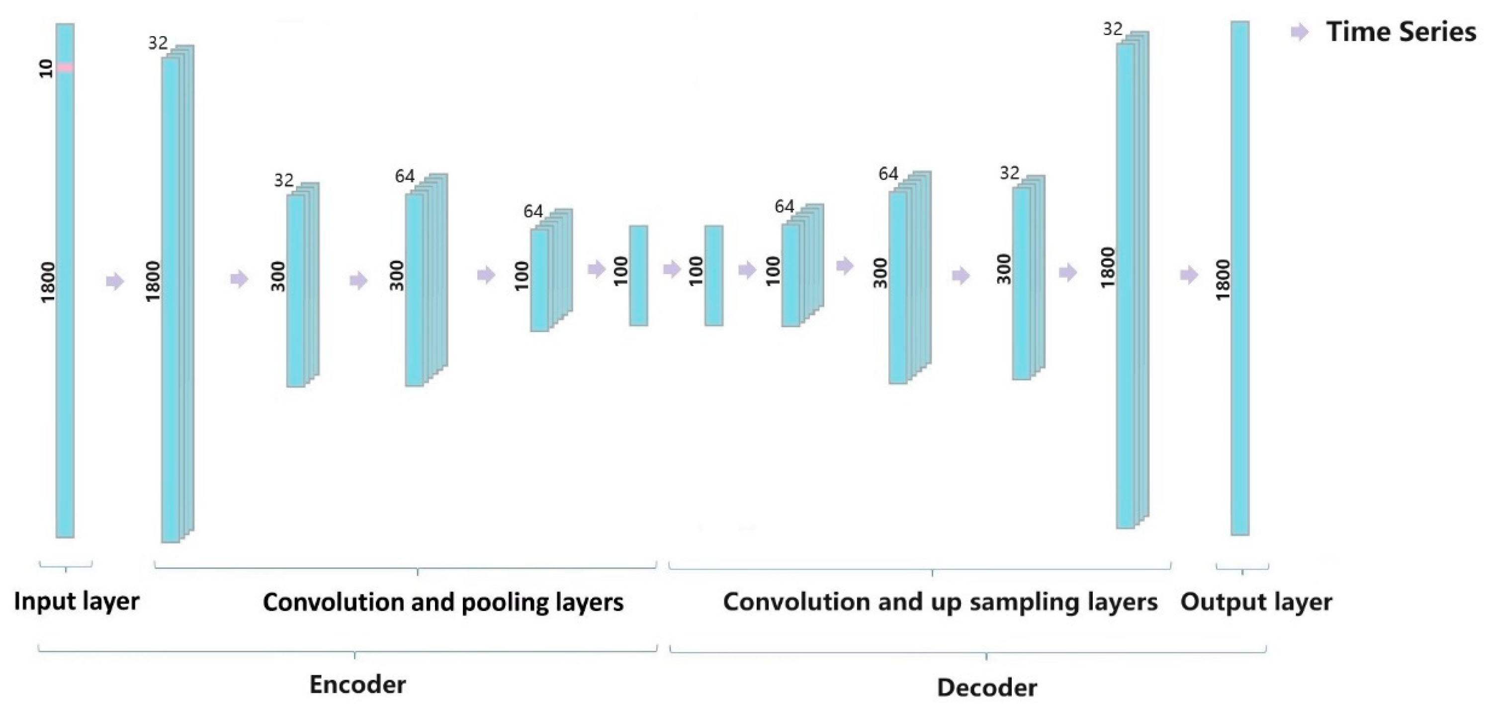
The CAE model typically involves the following main steps, as shown in Figure 5. First is the encoder part, where data are gradually reduced in dimension and essential features are extracted through a series of convolutional layers and pooling layers. This process can be seen as data compression and feature extraction. Then comes the decoder part, which follows the encoder and works to gradually restore the data’s dimensionality through a series of deconvolutional layers and upsampling layers, ultimately reconstructing the original input data. The goal of the convolutional autoencoder is to minimize the difference between the reconstructed data and the original input data, using the backpropagation algorithm to adjust the weights and parameters of neurons to reduce this difference. After multiple training iterations, the model’s performance is gradually improved.

4. Results and Discussion

4.1. Feature Band Selection

4.1.1. QPWS

Before modeling, the spectral data were preprocessed using the Savitzky–Golay (SG) [34,35,36] and standard normalized variate (SNV) [37,38,39] algorithm to remove noise and background effects from the spectral data. Through leave-one-out cross-validation and sk cross-validation with 2-fold, 5-fold, and 10-fold configurations, we identified the optimal cross-validation approach for the current dataset. Leave-one-out exhibited an average F1-score of 93.69% but incurred a considerable execution time of 3838.82 s. In contrast, the F1-scores for sk 2-fold, 5-fold, and 10-fold cross-validation were 94.39%, 94.54%, and 95.72%, respectively. Additionally, their respective execution times were 10.81 s, 28.16 s, and 61.12 s. Notably, sk cross-validation demonstrated a pronounced advantage in terms of runtime over leave-one-out.

Within sk cross-validation, the differences in F1-score between 2-fold, 5-fold, and 10-fold configurations were marginal. However, the runtime efficiency of 5-fold cross-validation stood out compared to the 10-fold counterpart. Considering the potential for insufficient model generalization with 2-fold cross-validation, we elected sk 5-fold cross-validation as the optimal cross-validation strategy for the current dataset. QPWS was run using the data from the calibration set and the validation set. In each iteration, the sk algorithm was used to select 80% of the samples to build the PLS-DA calibration model, and the regression coefficients for each variable were recorded in an array. After each iteration, a coefficient matrix was obtained, and the selected bands were ranked based on this coefficient matrix for the next iteration.

Figure 6 shows the trend of the number of sampled variables and accuracy as the sampling iterations increase starting from QPWS. Through the percentile filtering, the number of samples starts to decrease rapidly, and then the rate of decrease becomes smaller. This is because as the dataset becomes larger, the long tail effect becomes more pronounced. As the dataset decreases in size, the long tail effect gradually contracts or even disappears. From the subgraph in Figure 6, you can see that accuracy shows a slow upward trend in the first 100 iterations due to the removal of many uninformative variables. After iteration 150, accuracy drops rapidly, which is caused by the loss of information due to the removal of some key variables. A total of 68 feature bands were selected (Figure 7), reducing the original 1951 bands by approximately 29 times.

4.1.2. PCA

When performing PCA feature extraction, if the number of principal components is too large, it can easily introduce noise and redundant data [40]. In this experiment, the first eight dimensions of the willow spectra data were selected as the principal components, and the cumulative variance contribution rate reached 99.63%. The specific contribution rates are shown in

Table 3. The contribution rates of the first eight principal components of PCA.

Principal Component	Contribution Rate/%	Cumulative Contribution Rate/%
1	83.91	83.91
2	9.85	93.76
3	2.65	96.40
4	1.23	97.63
5	0.87	98.50
6	0.66	99.16
7	0.33	99.49
8	0.14	99.63

. From Figure 8, it can be seen that PCA can roughly distinguish between origins, namely, the red, yellow, and blue ones. However, the red and blue origins are mixed at the edges and are challenging to differentiate. Therefore, it can be inferred from the figure that PCA dimensionality reduction does not yield very accurate predictive results.

4.2. Bayesian Optimization

As shown in Figure 9, there is a significant difference in the performance of the full-spectrum infrared 1D-CNN model under different parameter configurations. The accuracy difference between different parameter configurations is around 60%. This means that the choice of appropriate model parameters is crucial for the final performance in the infrared spectroscopy data classification. In most cases, the model’s performance is relatively poor under default parameter configurations with an accuracy of about 30%. This performance difference may be due to the complexity and diversity of the data as well as the various noise and interference factors in the spectral data.

However, it is in such situations that Bayesian optimization demonstrates its powerful role. Bayesian optimization not only captures differences in model performance effectively but also automatically selects parameter configurations to improve the model’s performance to a higher level.

Table 4. The results of Bayesian hyperparameter optimization.

Model Hyperparameters	Value
Convolutional filter size	57
Convolutional kernel size	3
Convolutional filter stride	2
L2 regularization	0
Average pool size	1
Dense units	218
Dropout rate	0.2
Learning rate	0.003

shows the best hyperparameter optimization results for the full-spectrum infrared spectroscopy. It is worth noting that the single-layer model performs the best in terms of performance. Setting the average pooling size to 1 indicates no pooling operation is performed. The reason behind this choice may be that not performing pooling can preserve more information, and considering the relatively small size of the dataset, this seems to be a reasonable automatic choice. At the same time, the L2 regularization parameter is set without restrictions to achieve optimal performance.

4.3. Model Comparison Results

The selection criteria for the optimal number of LVs were determined through sk-fold cross-validation on the calibration and tuning sets, ensuring the best number of LVs among different feature selection methods. This criterion typically guarantees better performance for the selected PLS-DA model. The best number of LVs for feature selections using the full spectrum, QPWS, and PCA is 25, 27, and 8, respectively.

As shown in

Table 5. Comparison of prediction results of different models.

Method	Feature Selection	Macro/Weighted Avg	Precision/%	Recall/%	F1-Score/%	Runtime/ms
1D-CNN	Full spectral range	macro avg	99.45	99.44	99.44	3496
		weighted avg	99.46	99.45	99.45
	QPWS	macro avg	96.77	96.68	96.67	966
		weighted avg	96.76	96.69	96.66
	PCA	macro avg	92.20	92.28	92.22	85
		weighted avg	92.19	92.27	92.21
PLS-DA	Full spectral range	macro avg	97.06	97.04	97.04	240
		weighted avg	97.04	97.01	97.01
	QPWS	macro avg	98.52	98.52	98.52	125
		weighted avg	98.51	98.51	98.51
	PCA	macro avg	80.47	80.73	80.58	15
		weighted avg	80.34	80.60	80.45

, the comparison results indicate that the PLS-DA model with QPWS feature selection is superior to the full spectrum PLS-DA model with a 1.5% increase in precision when compared to PLS-DA models, although the runtime has increased by 92% due to the reduced number of bands. QPWS outperforms PCA in terms of precision with an improvement of approximately 18%, demonstrating a clear advantage over PCA.

In the comparison with the 1D-CNN model, the full spectrum results are superior to those with QPWS feature selection with PCA yielding the poorest results. The improved performance of the full spectrum over QPWS-selected results is attributed to the ability of deep learning models to automatically learn the most useful feature representations from raw data. When using 1D-CNN with the full spectrum, the model automatically reduces the weights of unimportant bands and increases the weights of important ones, effectively simulating a feature selection process. However, the full spectrum’s runtime is significantly slower than that of QPWS, differing by approximately 261%.

Comparing 1D-CNN and PLS-DA models together reveals that for both the full spectra and PCA dimensionality reduction, the 1D-CNN model outperforms PLS-DA with a difference in precision of approximately 2.4% and 12%, respectively. However, the QPWS-selected 1D-CNN model falls short of PLS-DA, which is possibly due to the loss of some effective features for the non-linear 1D-CNN model after PQWS feature selection. Additionally, the small dataset size might contribute to the machine learning methods performing better in this case compared to deep learning methods.

4.4. Optimizing the Model Using CAE

From Section 4.3, it can be observed that QPWS slightly underperforms in the 1D-CNN, although it significantly outperforms full-spectrum spectra in terms of speed. Based on this, we proposed a strategy for utilizing discarded spectral bands. After feature selection, the spectral bands that were not selected are further utilized. Specifically, the unselected bands are subjected to feature compression using CAE. Subsequently, the compressed bands were merged with the selected bands to be jointly used in model construction. The idea behind this strategy is that feature selection has already captured the linearly correlated essential bands, while CAE models can extract features containing non-linear information from the unselected bands. The CAE model parameters are configured as shown in Figure 10. In this figure, each block consists of three layers: the first layer represents the block’s number, the second layer represents the operation performed by the block (e.g., “Conv1D” indicates a convolution operation), and the third layer indicates the output dimension after the operation. The arrows represent the flow of input data. It can be seen from the figure that the dashed lines share the same shape, so this model is not only a CAE but also a stacked autoencoder model. This combination helps enhance the feature extraction capability of CAE. By performing multi-level feature learning, it strengthens the model’s understanding of abstract features. The CAE model is trained on the calibration set. Once the training is complete, features from the unselected spectral bands are extracted from the CAE model and merged with the bands selected through feature selection for further model construction.

The results from executing 1D-CNN on the integrated data are shown in Figure 11. Figure 11A,C depict the accuracy and loss during the execution of the integrated spectral bands, while Figure 11B,D represent the accuracy and loss for the QPWS spectral bands. It is evident from the figures that both models have mostly converged after 80 convolution iterations. However, during iterations 400–500, QPWS spectral bands continue to show fluctuations, whereas the integrated data exhibit very minor fluctuations and lower loss. To ensure consistency and reduce variation due to differences in each 1D-CNN iteration, we calculated the average accuracy and loss for iterations 400–500.

The average values for the integrated data and QPWS during iterations 400–500 are as follows:

• Calibrated accuracy: integrated data—99.41%, QPWS—96.61%;
• Tuning accuracy: integrated data—98.31%, QPWS—96.18%;
• Calibrated loss: integrated data—0.02, QPWS—0.09;
• Tuning loss: integrated data—0.04, QPWS—0.1.

The results clearly favor the integrated data. The final confusion matrix for the test set is presented in Figure 12. The accuracy for the test set is much higher for the integrated data at 99.9% compared to QPWS at 96.68%. Furthermore, the integrated data execution is significantly faster with a runtime of 1530 ms compared to QPWS’s 996 ms. The integrated data execution is approximately 228% faster than the full spectrum with 3496 ms.

Additionally, the study compared the results of a model using only the CAE algorithm, which reduced the number of wavelengths to 190 from the full spectrum, exceeding the 168 wavelengths used for the integrated data. The results, as shown in Figure 11C, indicate that the model performs well with a test accuracy of 96.69%. However, it still lags slightly behind the integrated data. This is attributed to feature selection choosing the most relevant linear features, which are then augmented with CAE for learning nonlinear features. This combination of feature learning helps the model better capture complex relationships in the data, resulting in improved performance.

4.5. Salix Psammophila Decision System

As shown in Figure 13, we have successfully developed a decision system based on near-infrared spectroscopy for willow in our research. The spectroscopic data are processed in two different ways: SNV and raw spectra. The effectiveness of these two preprocessing methods is reflected in the decision system. We used three different internal models for performance evaluation: the 1D-CNN with full wavelength, the 1D-CNN with integrated data, and PLS-DA after QPWS.

These models have been pre-trained and integrated into the decision system. In terms of system application, we adopted a model fusion strategy by weighting the results of the three internal models to obtain the final decision. This strategy is similar to boosting, where the full 1D-CNN and the integrated 1D-CNN each have a 40% weight, while the feature-selected PLS-DA has a 20% weight, which is assigned based on their respective accuracies and can be dynamically adjusted manually during the application process. The final decision result is determined based on these weight allocations to ensure the model result with the highest percentage is selected (Figure 14).

4.6. Model Validation

We collected hyperspectral data of Salix psammophila from the National Germplasm Repository in China and conducted performance validation of the model. A total of 109 spectral data were gathered from 13 provenance locations. Due to the relatively limited dataset, we implemented data augmentation techniques, expanding the dataset by a factor of 10, and then partitioned it into training and testing sets at a ratio of 3:1. The hyperspectral images are depicted in Figure 15 with the model’s performance results presented in

Table 6. Comparison of prediction results for hyperspectral data across different models.

Method	Feature Selection	Macro/Weighted Avg	Precision/%	Recall/%	F1-Score/%	Runtime/ms
1D-CNN	Full spectral range	macro avg	85.70	84.34	83.83	1530
		weighted avg	85.63	84.25	83.74
	QPWS	macro avg	83.31	80.77	80.40	362
		weighted avg	83.44	80.59	80.36
	integrated data	macro avg	92.75	91.28	91.06	458
		weighted avg	92.86	91.11	91.02
PLS-DA	Full spectral range	macro avg	35.28	27.78	26.15	59
		weighted avg	33.45	28.57	26.24
	QPWS	macro avg	36.11	31.94	27.91	13
		weighted avg	33.93	32.14	27.55
	PCA	macro avg	80.47	80.73	80.58	15
		weighted avg	80.34	80.60	80.45

.

Upon examination of the table, it is evident that compared to PLS data utilizing the full spectrum, the data after QPWS feature selection exhibited superior performance. However, the F1-score is relatively lower, which is possibly attributed to inaccuracies in the collection of hyperspectral data. Conversely, the performance of the 1D-CNN model surpassed that of the PLS algorithm. Within the 1D-CNN model, the spectral bands processed through QPWS and discarded bands using CAE fusion demonstrated outstanding performance, achieving an F1-score of 91%. The full spectrum followed, while QPWS had the least favorable effect.

In conclusion, when dealing with near-infrared and hyperspectral data, the approach of fusing processed spectral bands, especially utilizing QPWS and discarded bands through CAE fusion, proves to be more effective, particularly excelling in provenance classification tasks.

5. Conclusions

In this study, a novel feature selection algorithm called QPWS was initially developed for qualitative analysis. Subsequently, Bayesian optimization was employed to select the optimal 1D-CNN model, followed by feature selection and dimension reduction in unselected spectral bands using CAE, which were then fused to form new integrated data. Finally, the Salix psammophila decision system was established. The results indicate the following:

• The proposed QPWS algorithm has greater potential in the field of qualitative analysis compared to traditional algorithms, enabling the selection of more relevant important spectral bands;
• Bayesian optimization is a simple and effective method for selecting hyperparameters, particularly when there are numerous hyperparameters to consider;
• The integrated data outperform feature-selected data in 1D-CNN models.

These findings demonstrate that the approach employed in this study has significantly improved the classification of Salix psammophila origins based on Vis-NIR, providing valuable insights and methods for addressing similar problems.